

Abstract
Multivariate connectivity and functional dynamics have been of wide interest in the neuroimaging field, and a variety of methods have been developed to study functional interactions and dynamics. In contrast, the temporal dynamic transitions of multivariate functional interactions among brain networks, in particular, in resting state, have been much less explored. This article presents a novel dynamic Bayesian variable partition model (DBVPM) that simultaneously considers and models multivariate functional interactions and their dynamics via a unified Bayesian framework. The basic idea is to detect the temporal boundaries of piecewise quasi‐stable functional interaction patterns, which are then modeled by representative signature patterns and whose temporal transitions are characterized by finite‐state transition machines. Results on both simulated and experimental datasets demonstrated the effectiveness and accuracy of the DBVPM in dividing temporally transiting functional interaction patterns. The application of DBVPM on a post‐traumatic stress disorder (PTSD) dataset revealed substantially different multivariate functional interaction signatures and temporal transitions in the default mode and emotion networks of PTSD patients, in comparison with those in healthy controls. This result demonstrated the utility of DBVPM in elucidating salient features that cannot be revealed by static pair‐wise functional connectivity analysis. Hum Brain Mapp 35:3314–3331, 2014. © 2013 Wiley Periodicals, Inc.
Keywords: functional interaction, dynamics, Bayesian graphic models
INTRODUCTION
Functional segregation and integration are two general principles of the human brain architecture [Friston, 2009], and thus studying functional brain connectivity or interaction [Friston, 1994] based on functional magnetic resonance imaging (fMRI) data has received substantial interest. In the literature, a variety of computational and statistical methodologies have been developed to infer functional and/or effective connectivity [e.g., Friston, 1994; Zhou et al., 2009; Seth, 2010] and functional interactions [e.g., Chang and Glover, 2010; Deng et al., 2012; Marrelec et al., 2006; Ramsey et al., 2011; Smith et al., 2011]. In particular, in addition to the widely‐used pair‐wise correlation based functional connectivity analysis [e.g., Fox and Raichle, 2007; Honey et al., 2007; Li et al., in press], a variety of multivariate approaches, such as the dynamic causal modeling (DCM) [Friston, 2003], the multivariate autoregressive model (MAR) [Harrison et al., 2003], the structural equation modeling (SEM) [Protzner and McIntosh, 2006], Granger Causality Analysis [Deshpande et al., 2011] and the joint MAR‐SEM model [Kim et al., 2007], have been introduced to examine multiple nodes/networks simultaneously. More recently, a series of studies have demonstrated that graphical causal models [Ramsey et al., 2011; Sun et al., 2012], or so called casual Bayes nets, exhibit superior performance in identifying effective connections from real or simulated fMRI data. For instance, it has been shown [Ramsey et al., 2011; Sun et al., 2012] that the graphical causal models can effectively deal with several key problems in modeling effective connectivity such as inferring robust causal structures across individuals and handling varying delays in fMRI blood oxygen level dependent (BOLD) responses. Conceptually, multivariate graphical causal models based on Bayesian networks benefit significantly from simultaneous consideration of the whole network for functional interaction inference and being less sensitive to noise in the fMRI BOLD signals [Ramsey et al., 2011; Sun et al., 2012]. In general, multivariate models of functional connectivity or interaction have received increasing attention in the neuroimaging field.
Meanwhile, another important yet challenging issue that has received intensive recent interest is the temporal dynamics of functional connectivity. In many previous studies [e.g., Fox and Raichle, 2007; Honey et al., 2007; Li et al., in press], the functional/effective connectivity mapping approaches traditionally assumed temporal stationarity. That is, functional/effective connectivities or functional interactions were computed over the entire fMRI scan, which were then used to characterize the strengths or directionalities of connections across brain regions. However, there is mounting evidence from other authors [e.g., Bassett et al., 2011; Chang and Glover, 2010; Deco and Jirsa, 2012; Deshpande et al., 2008; Freyer et al., 2009; Ghosh et al., 2008; Lindquist et al., 2007; Majeed, et al., 2011; Robinson et al., 2010; Smith et al., 2012] and ourselves [Deshpande et al., 2006; Hu et al., 2011; Li et al., 2011, in press; Lim et al., 2011] indicating that functional/effective connectivities are undergoing dynamic state changes at different time scales. At a more basic level, neuroscience research suggests that the function of any cortical area is subject to top‐down influences of attention, expectation, and perceptual task [Gilbert and Sigman, 2007]. For instance, dynamic interactions between connections from higher‐ to lower‐order cortical areas and intrinsic cortical circuits mediate the moment‐by‐moment functional switching in brain. Even in resting state, the functional connectivity is still undergoing dynamic changes within time scales of seconds to minutes [e.g., Chang and Glover, 2010; Li et al., 2011, in press; Smith et al., 2012].
There has been exciting advances in both modeling multivariate functional connectivity/interaction [Friston 2003; Harrison et al., 2003; Kim et al., 2007; Protzner and McIntosh, 2006; Ramsey et al., 2011; Sun et al., 2012] and detecting temporal brain dynamics [Chang and Glover, 2010; Li et al., 2011, in press; Smith et al., 2012]. Recently, there are several literature reports that utilized the sliding time window based framework to investigate the functional brain dynamics [Allen et al., 2012; Li, et al., 2013], as well as works that used graphical modeling methods to detect change point in brain functional connectivity based on regression tree results by sparse regression between regions of interests (ROIs). However, it is important and much needed for an integrated framework to infer the representative signature patterns of the multivariate functional interactions and to quantitatively characterize the temporal transitions of those signature patterns simultaneously. Considering that functional brain activities are essentially network behaviors, we are motivated to develop novel computational and statistical approaches to investigate the temporal dynamics of multivariate functional interactions among brain networks, in order to elucidate interesting features that cannot be revealed by multivariate or non‐stationary methods alone, nor by static pair‐wise functional connectivity analysis.
Inspired by the success of Bayesian graphical causal models in neuroimaging [e.g., Ramsey et al., 2011; Smith et al., 2011; Sun et al., 2012] and in recognition of the importance of revealing dynamics of functional interaction patterns [e.g., Bassett et al., 2011; Chang and Glover, 2010; Hu et al., 2011; Li et al., 2011, in press; Lim et al., 2011; Majeed, et al., 2011; Smith et al., 2012], in this article, we propose and present a novel dynamic Bayesian variable partition model (DBVPM) that simultaneously infers global functional interactions within brain networks and their temporal transition boundaries. A key conceptual novelty in DBVPM is that the temporal boundaries of functional brain activities represented by fMRI time series are defined and determined by the abrupt change points of multivariate global chain and V dependences among networks, instead of the fMRI time series changes [Gao and Yee, 2003; Lindquist et al., 2007; Morgan et al., 2004], pair‐wise functional connectivity changes [Li et al., in press], or multivariate regression model [Cribben et al., 2012]. The major methodological novelty is that the temporal stationarity of functional interaction patterns within each time segment is achieved automatically and the temporal boundaries of successively different multivariate functional interaction patterns are statistically inferred naturally within a unified Bayesian framework. The DBVPM was evaluated and validated with simulated and experimental datasets, demonstrating its performance and robustness.
As a brief demonstration of potential application of DBVPM, the temporally segmented functional interaction patterns within the default mode network (DMN) [Fox and Raichle, 2007; Greicius et al., 2004; Raichle et al., 2001] and emotion [Sabatinelli et al., 2009] network derived from a post‐traumatic stress disorder (PTSD) dataset were clustered into representative signature patterns via effective dictionary learning methods [Yang et al., 2011]. The results revealed substantially different multivariate functional interaction signatures and temporal transitions in the default mode and emotion networks of PTSD patients, in comparison with those in healthy controls. This result demonstrated the effectiveness and utility of DBVPM in elucidating interesting features that cannot be revealed by traditional static pair‐wise functional connectivity analysis. The rest of this article is organized as follows. Method's section details the DBVPM and identification of representative signature patterns. Experimental setups and results are presented in Result section. Discussion and Conclusion section discusses limitations and possible future works, and concludes the article.
METHODS
Dynamic Bayesian Variable Partition Model
Preliminaries of Bayesian inference
Given y 1, y 2, …, y m iid (independent and identically distributed) observations from the d‐dimensional multivariate normal distribution
where μ denotes the d‐dimensional mean vector and Σ denotes the covariance matrix. Then the conjugate prior distribution of is the [Gelman et al., 2003] with the following form:
The posterior distribution of based on the data y 1, y 2, … , y m is the same type of , where
Here, S is a matrix.
Because we are interested in the posterior distribution of the configuration, we calculate the marginal distribution of the data y 1, y 2, …, y m as follows [Gelman et al., 2003]:
| (1) |
where is the multivariate gamma function:
We call the function defined in Eq. (1) as F(.), which will be used in the following calculations.
Chain‐dependence model
We say that a group of d normally distributed variables Y G = {Y1, … ,Yd} (G={1,…,d}) follows a chain‐dependence model if the index set G can be partitioned into three nonoverlapping subgroups A, B, and C such that A and C are conditionally independent given B, as shown in Figure 1a, while only C is allowed to be empty, and A and B must contain at least one ROI.
Figure 1.

(a) Chain‐dependence model of the group of variables Y G. (b) V‐dependence model of the group of variables Y G. (c). Illustration of data matrix of Y G, where y i are the values of all ROIs at time i (the ith column in the matrix), and Y j are the values of the jth ROI at all times (the jth row in the matrix).
Under the chain‐dependence model, the joint probability of Y G could be decomposed and calculated as follows:
| (2) |
where is the joint probability of (Y i, Y j, …) as defined and will be calculated in Eq. (1). For calculating the posterior distribution function F(.), the time series (y 1, y 2,…,y m) defined in the ROI of each group (groups of rows in the data matrix) are used as the function input.
V‐dependence model
We say that d normally distributed variables Y G = {Y 1, … ,Y d} (G = {1,…,d}) follows a V‐dependence model if A and B are marginally independent, as shown in Figure 1b. In this case, C can be viewed as “children” of A and B, and the joint probability of YG could be decomposed and calculated as follows:
| (3) |
where is the joint probability of (Yi, Yj, …) as defined and will be calculated in Eq. (1).
Here, we choose chain and V dependences to model the global structure, instead of using a Bayesian network to model the detail structure [Neapolitan, 2004]. Essentially, these two structures can contain all the global structures for all the Bayesian networks (i.e., directed acyclic graph (DAG)). For example, suppose we have four ROIs with structure 1‐>2, 3‐>4, our method will find a V structure with 1 and 2 in A, 3 and 4 in B (or 3 and 4 in A, 1 and 2 in B, see Fig. 1b) and nothing in C. Because within each of A, B and C, we use the saturated model (complete graph, every ROI is connected with others), and chain structure and V structure model the global connectivities between three (local) groups of ROIs (A–C). Thus our dynamic Bayesian partition model is looking for change points that make big changes in global structure, not the small change in local structure. The global structure found by chain and V structure is an (asymptotically) inclusion model of the true DAG model (i.e., all the conditional independence in this global structure exist in the true DAG model, but not vice versa) [Chickering, 2002; Chickering and Meek, 2002; Heckerman et al., 1995].
Bayesian variable partition model (BVPM)
Given an ROI data matrix Y = (y 1, y 2, …, y m) in which y 1, y 2, …, y m are iid from the d‐dimensional multivariate normal distribution. Here, m denotes the number of observations (the number of time points in an fMRI signal) and d denotes the number of ROIs within a functional brain network, as illustrated in the sample matrix (Fig. 1c). We design a Bayesian variable partition model to infer the dependence structure (chain or V structure) among d ROIs.
Let S denote the dependence structure as chain (S = 1) or V (S = 0) structure. Given S, let denote the grouping (partition) of the index G = {1,…,d}) to subgroup A–C where means the jth ROI is grouped in subgroup k (k = 0 means A, k = 1 means B, k = 2 means C). Thus data matrix Y = (y 1, y 2, …, y m) are our observed data, while S and are unknown parameters of interest. The likelihood is which is calculated as Eq. (2) when S = 1, and Eq. (3) when S = 0. The prior and , and uniform priors are used for both and . Thus the posterior distribution is , and Markov chain Monte Carlo (MCMC) (Metropolis‐Hastings) (Liu, 2001) are designed to sample from the posterior distribution with the following proposals:
Randomly choose one ROI and change its subgroup membership;
Randomly choose two ROIs and switch their subgroup memberships;
Swap the values of S (either from 0 to 1, or from 1 to 0).
Dynamic Bayesian variable partition model
Given an ROI data matrix Y = (y 1, y 2, …, y m) (here m denotes the number of observations in the temporal order and d denotes the number of ROIs), we are interested in whether there are underlying differences in the dependency structures among the d ROIs between different time periods and where are the boundaries of temporal blocks that exhibit significant differences from each other. Once these boundaries are determined statistically, they are considered as the change points of functional interaction patterns within the brain networks. In this article, we propose a dynamic Bayesian variable partition model (DBVPM) equipped with two‐level MCMC scheme that aims to infer the boundaries of temporal blocks and the variable dependency structures within each block simultaneously in a Bayesian framework. Figure 2 illustrates the basic ideas of the proposed DBVPM, in which two temporal change points partitioned three fMRI time series into three different functional interaction patterns.
Figure 2.

Illustration of two temporal change points of functional interaction patterns at time point 1 and 2. In the time period before change point 1, the functional interaction among three fMRI signals is a Chain‐dependence model (e.g., signal 1 ‐> signal 2 ‐> signal 3), while between time points 1 and 2, it is a V‐dependence model (e.g., signal 1 ‐> signal 2 <‐ signal 3). After the time point 2, it is again a V‐dependence model (e.g., signal 2 ‐> signal 1 <‐ signal 3). [Color figure can be viewed in the online issue, which is available at http://wileyonlinelibrary.com.]
Define a block indicator vector
where I i = 1 if the ith observation (y i) is a change point (defined as the starting point of a temporal block), and I i = 0 otherwise. Therefore, the m temporal observations were segmented into totally blocks, as the first change point is always the starting time point and the number of change points segmenting the observations is . In each block, the variables follow (unknown) either the chain‐dependence model or V‐dependence model. We introduce the structure indicator vector
where S b = 1 if the b‐th block follows the chain‐dependence model, and S b = 0 if the b‐th block follows the V‐dependence model. Moreover, the variables in each block will be partitioned into three subgroups A–C. We introduce a partition indicator vector:
where with is the partition indicator vector of the b‐th block. The marginal likelihood of the data matrix Y = (y 1, y 2, …, y m) can be represented as follows
in which could be calculated according to Eqs. (1), (2), (3). Here, the DBVPM simultaneously models and characterizes high‐order functional interactions and their temporal dynamics via a unified Bayesian framework. Notably, in the above DBVPM, the statistical independence among the temporal segments is assumed here, which is practically critical to solve the above equation. Therefore, the posterior distribution of the configuration can be easily obtained since
where . We used uniform prior for and .
Two‐level MCMC scheme
In this section, we propose a two‐level Metropolis‐Hastings (MCMC) [Liu, 2001] scheme to sample from the posterior distribution of the block boundaries and dependency structures within each block. In the proposed scheme, the lower level MCMC samples from the posterior distribution of the dependency structures of each block given the block boundaries, and the higher level MCMC samples from the posterior distribution of the block boundaries. Specifically, in the lower level MCMC, the proposal scheme involves alternating between the chain and V structures and changing the group labels of each variable. The likelihood can be calculated using the formula [Eq. (1), (2), (3)] described in previous sections. In the higher level MCMC, the proposal scheme involves segmenting one block into two, merging two neighboring blocks and shifting a block boundary. In each higher level step, every block runs through a lower level MCMC. A dependency structure is sampled for each block as the dependency structure for that block in the higher level proposal. Then the log likelihood of the proposal can be calculated by summing up the log likelihood of each block. We then check the mixing of MCMC and exclude the burn‐in from the actual MCMC sample of the posterior distribution. Then the posterior probability for each time point (1, 2,…,m) to be a change point was calculated from MCMC samples. A running example of how the DBVPM reveals the dynamics of functional interaction patterns is provided in Supporting Information Fig. 1.
Functional interaction pattern classification and temporal finite‐state machines
The DBVPM was applied on the resting state fMRI (R‐fMRI) signals extracted from both the default mode network (DMN) and emotion networks in 98 brains (53 healthy controls and 45 PTSD patients). Additional details of the subject recruitment, neuroimaging parameters, and localizations of the default mode and emotion networks are provided in Supporting Information. In brief, we first defined the R‐fMRI signals on our recently developed and validated 358 consistent and corresponding DTI‐derived landmarks across multiple brains and populations, named dense and individualized common connectivity‐based cortical landmarks (DICCCOL) ROIs [Zhu et al., 2011a, 2011b, 2012] (The source codes and data models have been released online at: http://dicccol.cs.uga.edu). Then, we used the functionally labeled DICCCOLs and their prediction models to locate the default mode network (DMN) [Fox and Raichle, 2007; Greicius et al., 2004; Raichle et al., 2001] and emotion [Sabatinelli et al., 2009] network. In total, we obtained 2,335 quasi‐static temporal segments of functional interaction patterns in the default mode network and 1,567 segments in the emotion network from the 98 subjects by using DBVPM.
Because the two brain networks were localized by the DICCCOL system which already established the correspondences of network nodes across individuals, we can congregate the functional interaction patterns from different brains and perform statistical modeling of common interaction patterns. Without loss of generality, we used the DMN as an example to showcase the algorithmic pipeline for preprocessing and inference of representative functional interaction patterns. First, since the identified function interaction patterns are binary and could be affected by noise, we used the Fisher discriminative dictionary learning algorithm [Yang et al., 2011] to seek a dictionary D describing the 2,335 function interaction patterns defined in each temporal segment in the DMN, by minimizing the energy function in the equations:
| (4) |
where
| (5) |
and
| (6) |
where A contains the vectorized functional interaction patterns of all the quasi‐static temporal segments, which is a 64 × 2,335 matrix as the DMN consists of 8 DICCCOL ROIs and its functional interaction pattern is an 8 × 8 matrix. X is the encoded matrix A based on the learned dictionary D. In Eq. (4), r(A, D, X), is the constraint on discriminative fidelity, thus making the dictionary D able to code the data with minimum residual and ensuring that the coding should only use one sub‐dictionary D i, but not other sub‐dictionaries. The second term λ1||X|| in Eq. (4) is the sparsity constraint [Yang et al., 2011], requiring the coding coefficient X be as sparse as possible, i.e., the total number of nonzero items in X should be minimized. The third term f(X) in Eq. (4) is the constraint on the discriminative coefficient [Yang et al., 2011], which aims to minimize within‐class scatter of X and maximize the cross‐class scatter of X, according to the Fisher discrimination criterion [Yang et al., 2011]. This constraint can make the coding coefficient X to be discriminative.
In Eq. (5), X i is the encoding result of A i, which is one of the classes of data A, based on the whole dictionary D. Thus the first term in Eq. (5) is the overall residual of using dictionary D to encode A i. X i i is the encoding of A i on sub‐dictionary D i, which is the specific sub‐dictionary in correspondence with A i. Thus the second term in Eq. (5) is the residual of using only part of the dictionary to encode A i. X i j is the encoding of A i on other sub‐dictionaries D j other than D i, and it would be minimized because we only wish to use the correct dictionary D i to encode it. In Eq. (6), c is the total number of classes in A, as well as the total number of sub‐dictionaries in dictionary D, while n i is the number of items in the projected data X i, as there are multiple items in each class. λ 1, λ 2 and η are the trade‐off parameters.
During the learning process, the learned dictionary D was constrained to consist of 12 subdictionaries (corresponding to the subsequent 12 labels for the function interaction patterns). To find the optimized number of subdictionaries to encode the interaction patterns and avoid model over‐fitting, we used various numbers of classes ranging from 5 to 20 to encode the input data A. It was found that the encoding residual was decreasing monotonically with more numbers of sub‐dictionaries, and the minimum number of dictionaries that could encode over 95% of the input data (i.e. encoding residual less than 5%) was 12. Then, we used the center of each sub‐dictionary (which are 12 matrices with dimension of 8 × 8) to encode the original 2335 8*8 interaction segment matrices, in order to remove the noise:
| (7) |
In the above equation, we performed linear regression between the function interaction patterns and the center of each subdictionary, and the regression coefficients were used to obtain a linear combination of subdictionaries in expressing the original data while removing the regression residual ε.
In this work, we have applied the above dictionary learning method to all of the pre‐processed functional interaction patterns in the DMN and emotion network to derive the representative signature patterns. It turned out that we can identify a number of meaningful patterns (12 for both DMN and emotion networks) that account for a majority of the temporal interaction segments. In particular, these common patterns are reproducible across populations, and they were defined as the representative signature patterns of functional interactions. Finally, each temporally segmented interaction pattern was assigned to one of the signature patterns by the largest regression coefficient obtained in Eq. (7), and their temporal transition patterns within each individual and across subjects were modeled by a finite‐state machine [Black, 2008], which will be shown in Representative Functional Interaction Patterns and Temporal Transitions section.
RESULTS
Evaluation of the DBVPM model on simulated data
We used two simulation methods and the associated datasets to evaluate and validate the DBVPM models. In the first method, we used statistical models to generate interacting time series with dynamically changing structures (iid within each quasi‐stable segment). Specifically, we simulated six sets of interaction models with different levels of complexities, ranging from 3 nodes to 10 nodes and ranging from single chain‐dependence structure to more complex ones. Figure 3 illustrates the temporally changing interaction structures in the six interaction models (top panels) and the posterior probability for each time point as the change point (bottom panels). For instance, shown in Figure 3a, there are 3 nodes (ROIs, Y 1, Y 2, and Y 3) and 200 time points that are divided into two blocks at time point 101. The simulated data is generated as follows: all the three ROIs are marginally N(0,1). From time points 1 to 100 (the first block), all the three ROIs are independent of each other. From time point 101 to 200 (the second block) the structure is a chain structure: Y 2‐>Y 1‐>Y 3, with correlation coefficients , as shown in the top panel of Figure 3a. For another example, in Figure 3e, there are 10 ROIs (Y 1 to Y 10) and 200 time points that are divided into 2 blocks at 101. The simulation data is generated as follows: all the 10 ROIs are marginally N(0,1). From time point 1 to 100 (the first block), all the five pairs of 10 ROIs are independent of each other. Within each pair, two ROIs are ∼N(0, Σ), . For the second block (from 101 to 200), the structure is a star‐like structure, with Y1 being the center and other ROIs (Y 2 to Y 10) dependent on it with correlation coefficient . This star‐like structure means given Y1, all other ROIs (Y 2 to Y 10) are conditionally independent of each other. It is interesting that our DBVPM successfully detected all of the simulated changes of interaction patterns in all of the models, as shown in each of the bottom panels in Figure 3a–f. It is striking that both of the model sensitivity and specificity of DBVPM in this experiment are 100%, indicating the good performance of DBVPM. Further, we have repeated the simulation for 100 times, and the averaged Type I error rate over all six types of simulations is 1.83%, and the averaged Type II error rate is 1.67%.
Figure 3.

The dynamics of interaction pattern (top) of the simulation data using the first method and the change point detection result (bottom, the posterior probability for each time point as a change point) of DBVPM model in six different models, depicted in (a–f), respectively. Nodes Y1‐Y10 correspond to the generated ROIs and the arrows connecting them show the directed interaction between them (Bayesian network structure). In each model, the interaction pattern between simulated ROIs would change as indicated by the bold red lines separating the blocks, and the numbers on those red lines show the time of the change. The change point detection results are visualized as the value of posterior probabilities at each time point obtained by DBVPM, where a high value indicates high probability for state change. It should be noted that the time lengths of the simulated signals are not same through the six simulations. [Color figure can be viewed in the online issue, which is available at http://wileyonlinelibrary.com.]
In the second simulation method, the nodes were modeled as the neurons in the neural networks and the interaction between them were simulated as the coupled neuronal spiking (firing), and thus there are some temporal dependency within each quasi‐stable segment (compared with the iid case in the first simulation method). The neuron spiking model was introduced in [Izhikevich, 2003, 2004], where the time series of each node generated by this method is the oscillation of the membrane potential of neuron in a network, which follows the equation described in [Izhikevich, 2003]. Similar to the first simulation method, we generated nine sets of time series on five nodes according to the different dynamic interaction patterns defined in nine models, as visualized in Figure 4. We repeated the simulation for 100 times, and the average Type I and Type II error rates over nine models were 5 and 7.78%, respectively, where the threshold of posterior probability was set as 0.99.
Figure 4.

The dynamics of interaction pattern (top) of the simulation data using the second method and the change point detection result (bottom, the posterior probability for each time point as a change point) of DBVPM in nine different models, depicted in (a)–(i), respectively. Nodes N 1‐N 5 are the interacting neurons in the neural network, each with the generated time series characterizing its membrane potential. The arrows connecting them show the undirected interaction between these nodes. Similar to Figure 3, the interaction pattern changes are indicated by the bold red lines separating the blocks, and the numbers on those red lines show the time of the change. At the bottom of each model is the plot of the value of posterior probability for each time point as a change point obtained by DBVPM. It should be noted that the time lengths as well as the position(s) of the change points of the simulated signals are not same through the nine simulations. [Color figure can be viewed in the online issue, which is available at http://wileyonlinelibrary.com.]
Evaluation of the DBVPM Model on Experimental Data
To evaluate the change point detection accuracy of the proposed DBVPM in Dynamic Bayesian Variable Partition Model section on experimentally acquired fMRI data, we visually identified the temporal boundaries of functional interaction patterns for 98 subjects with multimodal R‐fMRI and DTI data, as illustrated in Figure 5a. The details of the neuroimaging data acquisition and preprocessing are provided in the Supporting Information. Given the lack of ground‐truth in experimental R‐fMRI data, this semi‐automatic visual delineation of temporal boundaries was used for algorithm evaluation. Here, the total functional interaction strength of each DICCCOL has been summed together among all of its connections to other DICCCOLs. It is evident that there are clear functional interaction pattern changes along the temporal axis, as highlighted by the dashed black lines in Figure 5a. These boundaries were independently verified for all of the 98 subjects we studied in this article, and were used as the benchmark data for algorithm accuracy evaluation. Based on the above benchmark segmentation, Figure 5b shows the evaluation results of DBVPM for the emotion network. It is evident that given a marginal difference of the six time points, the results by DBVPM and those by the interactive labeling have quite high probability of agreements. The average agreement for the emotion network for all of the 98 subjects was 0.9142, which is considered as quite accurate. This result demonstrates the good accuracy of DBVPM in segmenting temporally varying functional interaction patterns within brain networks. Furthermore, the temporal transitions of functional interactions within the DMN were identified interactively for twenty randomly selected cases and then compared to the change points obtained by DBVPM. It turned out that the average difference between the interactively‐labeled change points and those by DBVPM is 3.5 time points, and over 90% of the interactively‐labeled change points are within 10 time‐points neighborhoods of those by DBVPM. This result further demonstrates that the DBVPM is accurate in identifying temporal functional interaction transitions in experimental R‐fMRI data.
Figure 5.

(a) Illustration of the temporal dynamics of functional interactions within brain networks. The horizontal axis indicates time, and the vertical axis indicates the 358 DICCCOLs with color indicating their functional interaction strength. Thus, each row represents the temporal dynamics of each DICCCOL's interaction strength, while each column is the functional interaction strength pattern of the whole brain represented by 358 DICCCOLs [Zhu et al., 2012]. The temporal boundaries (highlighted by dashed black lines) between different interaction patterns were visually determined and verified by experts. (b) Result on the emotion network. The horizontal direction is the difference between the interactively labeled change time point and the DBVPM‐derived time point. The vertical axis is the probability of the agreement with the results by two methods (DBVPM and interactive labeling). Each blue curve represents one subject. [Color figure can be viewed in the online issue, which is available at http://wileyonlinelibrary.com.]
To evaluate whether DBVPM can differentiate possible altered functional interactions and transition dynamics in brain diseases, we analyzed a clinical dataset that includes both PTSD and healthy controls (details in the Supporting Information). In this section, we compared the frequencies of the functional interaction pattern changes in the DMN and emotion network in both PTSD and control subjects. It turned out that there are no significant differences (p value > 0.05) between the change point frequencies in PTSD and those in controls, as demonstrated in Supporting Information Figure 3. This result suggests that the difference between PTSD patients and controls might lie in the functional interaction patterns and their temporal transitions, instead of in the mere change point frequencies. Therefore, we further characterized the functional interaction and temporal transition patterns within PTSD and controls.
Representative Functional Interaction Patterns and Temporal Transitions
We applied the DBVPM on the datasets described in the Supporting Information, and found that the functional interaction patterns in the DMN can be clustered into 12 distinctive centers, which are matrices describing the functional interaction among eight DICCCOL ROIs in DMN, as shown in Figure 6. It is evident that in each distinctive cluster pattern, one or more DICCCOL ROIs have strong interactions with others and serves as the interaction inflow center, e.g., the DMN node ID #7 (left middle temporal gyrus) in pattern #1 and the DMN node ID #4 (right angular gyrus), #5 (left medial frontal gyrus) and #7 (left middle temporal gyrus) in pattern #4, as highlighted by the blue arrows. It is interesting that different DMN nodes serve as the functional interaction inflow centers in the 12 distinctive patterns, and the inflow node exhibits high‐order (e.g., 7th order in DMN node ID #7 in pattern #1) functional interactions with other nodes within the DMN. These results not only verified our hypothesis that there exists high‐order functional interactions within brain networks (e.g., DMN), but also demonstrated that our DBVPM can effectively infer those high‐order interactions. Also, the results in Figure 6 demonstrated the complexity of high‐order functional interaction patterns in the DMN, although the neural basis of these patterns remains to be explained and interpreted in the future. It is emphasized that it is critical to employ the DICCCOL system that offers intrinsic correspondences of network nodes across individuals, such that the remarkably different functional interaction patterns within a relatively short period of 7 min R‐fMRI scans from different brains can be pooled, integrated and clustered at the population level.
Figure 6.

The visualization of functional interaction patterns in 12 clustered representative signature states from DMN. The details of DMN nodes are listed in Supporting Information Figure 2 and Supporting Information Table I. The functional interactions among DMN nodes are represented by the blue arrows. [Color figure can be viewed in the online issue, which is available at http://wileyonlinelibrary.com.]
Therefore, the cluster centers in Figure 6 are defined as the representative signature states of functional interactions for the DMN, and are indexed by order of the number of temporal segments clustered (i.e., their occurrence frequencies). For visual examination, the top 5 functional interaction signature states along with the temporal segments assigned to them are shown in Supporting Information Figure 4 via multidimensional scaling. It can be clearly seen that there are substantial differences among those different signature states, despite that the higher dimensional functional interaction patterns have already been reduced to only two dimensions. After the above dictionary learning procedure described in Functional Interaction Pattern Classification and Temporal Finite‐State Machines section, the temporal segments of functional interaction patterns in the DMN of all subjects (both PTSD and controls) were encoded into the same signature state space (12 representative states). Examples of the encoded functional interaction state changes of the DMN from three randomly selected healthy control subjects are shown in Supporting Information Figure 5. It can be clearly seen that the functional interaction patterns in the DMN change dramatically along the temporal axis, and particularly, the transition patterns vary significantly across different brains. This result replicated previous literature reports that the brain function undergoes significant temporal dynamics [e.g., Bassett et al., 2011; Chang and Glover, 2010; Majeed, et al., 2011; Robinson et al., 2010; Smith et al., 2012]. Furthermore, the results in Supporting Information Figure 5 suggest that the relatively short period of around 7 min resting state fMRI scan might only take a snapshot of the large‐scale space of possible temporal brain state transition patterns. Again, it is emphasized that it is essential to employ the DICCCOL system that offers intrinsic correspondences of network nodes across individuals, such that the remarkably different snapshots of temporal transition patterns of functional interaction within a short period of R‐fMRI scans from different brains can be aggregated, modeled and characterized at the population level.
To further interpret the encoded functional state changes, and to quantitatively characterize the brain state dynamics, we encoded the functional states in the DMN in two groups of subjects (normal controls and PTSD patients) by the same set of representative signature states listed in Figure 6, and examined the statistical distributions of the signature states respectively. For each of these two groups, the histogram of 12 representative signature states were obtained and investigated, as shown in Figure 7a. In the figure, we can clearly see substantial differences in several state distributions in normal controls and PTSD patients. For instance, the control subjects tend to have higher frequencies than PTSD patients (by 13%) in signature state #1, while the PTSD patients tend to have substantially higher frequencies in signature states #3 and #11, with differences of 28 and 34%, respectively. Based on the visualizations of functional interaction patterns in Figure 6, the neuroscience interpretation of higher frequencies in states #3 and #11 is that PTSD patents tend to fall more frequently in the brain states with intense functional interactions in both the left and right posterior cingulate gyri (DMN nodes #2 and #6 in Fig. 6), which is consistent with current neuroscience knowledge of PTSD [Francati et al., 2006].
Figure 7.

(a) Histogram of percentage of functional states assigned to each signature states in the DMN from normal control subjects (shown in blue) and patient subjects (shown in red). The error bars stand for the standard errors of the two histograms. (b–c) The probability of transition from each state to another (i.e., the finite‐state transition machine). The color of each cell indicates the frequency of the state transition from its row index to its column index. The values in the matrix have been normalized so that the sum of all cells is equal to 1, and the color bar is on the right. Visualization on the left (b) is from normal control group and the right (c) is from PTSD patient group. Five transition patterns with substantial difference between PTSD and control brains are highlighted by colored arrows. [Color figure can be viewed in the online issue, which is available at http://wileyonlinelibrary.com.]
Furthermore, we examine the temporal transition patterns of the functional interaction patterns. In this sense, the brain activity within the DMN can be regarded as a dynamic process that transits successively through a set of representative signature states S 1, S 2, S 3, …, Sn, which is akin to a finite‐state machine (totally 12 states) [Black, 2008]. Quantitatively, the transition from any states S i to its next state S j is represented by the probability P ij. Then, these probabilities obtained from the identified state changes as shown in Supporting Information Figure 5 are summarized and visualized in a 12 × 12 finite‐state transition matrix in Figure 7b–c. It can be easily seen that there are substantial differences between the transition patterns in PTSD and control brains, some of which are highlighted by the colored arrows. For instance, the black arrows show two transition patterns that are substantially more frequent in healthy brains than the PTSD brains, while the green, red and orange arrows point to transition patterns that are substantially more frequent in PTSD brains than healthy brains. It is interesting that although the total occurrence frequencies of state #2 in PTSD and control brains are very similar (Fig. 7a), their temporal transition patterns to state #2 are quite different (pointed by the green and black arrows in Figure 7b–c, where the cells pointed by the black arrows have an average difference of 40%, the cells pointed by the red arrows have 47% difference, and the cells pointed by the green arrow has 112% difference. Totally, there are 78 out of 144 (54.2%) transition cells that have differences larger than 30% between normal controls and PTSD patients. The finite‐state transition matrix can also be depicted as a visual diagram (Supporting Information Fig. 6), in which each state is represented as a node and the probability of transition is represented the edge strength. This result suggests the importance of revealing temporal transition patterns of functional interactions. However, the mechanisms underlying these functional state transitions are to be elucidated in the future.
Reproducibility Studies and Comparisons
To examine the reproducibility of the above functional interaction signature states and the finite‐state transition machines, we randomly split the temporally segmented functional interaction patterns in healthy brains into two equally sized groups. Then, the similar approaches were applied on these two separate groups of interaction patterns. Interestingly, the results visualized in Figure 8 demonstrated the very good reproducibility of the proposed methods. For instance, the distributions of the frequencies of the 12 signature states in subset 1 and subset 2 are quite similar. Also, the finite‐state transition patterns in Figure 8b,c are similar as well. These results demonstrated that the clustered 12 functional signature states are truly representative of the dynamic functional states of the DMN in healthy brains.
Figure 8.

(a) Histogram of percentage of interaction segments assigned to each signature states in the DMN from normal controls, which were split into two subsets with same number of subjects. The error bars show the standard errors of the two histograms. (b–c) The transition matrix from two groups of equal numbers of interaction patterns. The color of each cell indicates the frequency of the state transition from its row index to its column index. Values in the matrix have been normalized so that the sum of all cells is equal to 1. Visualization at the left (b) is from subgroup 1 and the right (c) is from subgroup 2. [Color figure can be viewed in the online issue, which is available at http://wileyonlinelibrary.com.]
In addition to the DMN, DBVPM was also used to analyze the emotion network of 53 normal controls and 45 PTSD patients (details in the Supporting Information). In total, the functional interaction patterns in the emotion network can be clustered into 12 distinctive centers, as shown in Figure 9. It is evident that in each distinctive cluster, one or more DICCCOL ROIs have much stronger interactions with others and serves as the interaction inflow center/centers, e.g., the emotion node ID #1 (left inferior temporal gyrus) in pattern #1 and the emotion node ID #9 (right lingual gyrus) and #11 (right lingual gyrus) in pattern #2, as highlighted by the blue arrows. It is interesting that different emotion nodes serve as the functional interaction inflow centers in the 12 distinctive patterns, and the inflow node exhibits high‐order (e.g., 13th order in emotion node ID #1 in pattern #1) functional interactions with other nodes within the emotion network. These results further verified our hypothesis that there exists high‐order functional interactions within brain networks and that our DBVPM can effectively infer those high‐order interactions. The results in Figure 9 additionally demonstrated the complexity of high‐order functional interaction patterns in the emotion.
Figure 9.
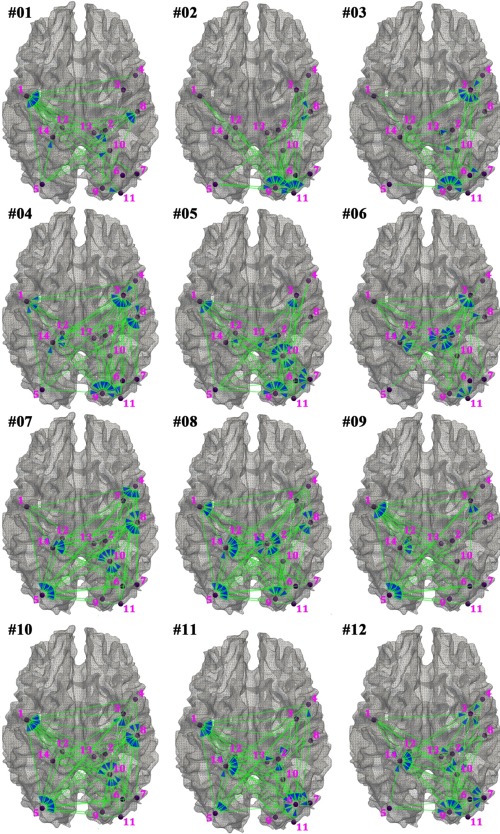
The visualization of functional interaction patterns in 12 clustered representative signature states for the emotion network. The details of emotion network nodes are listed in Supporting Information Figure 2 and Supporting Information Table I. The functional interactions among nodes are represented by the blue arrows, as similar to Figure 6. [Color figure can be viewed in the online issue, which is available at http://wileyonlinelibrary.com.]
The histograms of representative functional interaction patterns and the temporal finite‐state transition matrices within the emotion network are shown in Figure 10. In Figure 10a, it can be clearly seen that there are substantial state distribution differences between PTSD and healthy controls (on average: 30% difference; maximum: 56% difference). For instance, the control subjects tend to have substantially higher frequencies in signature states #6 and #9, while the PSTD patients tend to have substantially higher frequencies in signature states #1, #5, #7, and #11. In addition, the differences between the finite‐state transition machines (Figure 10b,c) are substantial. For instance, some of the significantly different transition patterns are highlighted by corresponding colored arrows. However, the neural basis of these differences is to be elucidated in the future. Additional quantitative comparisons of the PTSD and controls are provided in the Supporting Information.
Figure 10.

(a) Histogram of 12 states in emotion network in normal control subjects (shown in blue) and PTSD patient subjects (shown in red). The error bar represents the standard error of the two histograms. (b–c) Visualization of state transition matrices in emotion network in normal control (b) and PTSD patient subjects (c). The color of each cell indicates the frequency of the state transition from its row index to its column index. Values in the matrix have been normalized so that the sum of all cells is equal to 1. The color bar is on the right. [Color figure can be viewed in the online issue, which is available at http://wileyonlinelibrary.com.]
DISCUSSION AND CONCLUSION
We have presented a novel dynamic Bayesian variable partition model (DBVPM) to infer functional interaction pattern and its temporal transitions in the default mode and emotion networks that were localized via the DICCCOL system. Experimental evaluations have demonstrated the accuracy of the DBVPM method. In particular, our simulations with known ground‐truth showed that the dynamic Bayesian partition model can accurately identify change points for all types of global structures, even though we did not model the detailed local structure. Such strategy not only highlights the points of large changes in global structures and tends to ignore points of small change in local structures, but also eases the computational burden of our Bayesian method. Furthermore, we observed from simulations that the proposed model still inferred global structures of blocks accurately when the lengths of blocks were between 10 and 20 for most of the cases such as Figure 3a,b,d–f. In some rare case as Figure 3c, the smallest length of block needs to be greater than 50 to infer global structure accurately. However, even in the cases where the sample size was smaller than the required length, the DBVPM still detected change points accurately without perfect estimation of global structures of blocks. Once we accurately pinpoint the change points, we can always use all the structure learning methods which assume temporal stationary (like greedy equivalence search (GES) [Meek, 1997], Peter and Clark (PC) [Spirtes and Glymour, 1991], independent multiple greedy equivalence search (IMaGES) [Ramsey et al., 2011]) to learn the detail local structures.
Then, the inferred functional interaction patterns within the DMN and emotion network from a group of 98 PTSD and control brains were aggregated into a pool and were then classified into 12 representative functional states. It turned out that the distributions of the frequencies of these 12 states and their temporal finite‐state transition machines are reproducible across healthy control brains. The applications of these methods in the PTSD dataset demonstrated that PTSD exhibits substantial differences in terms of both distributions of state frequencies and transition patterns. In particular, our results demonstrated that the emotion network of PTSD subjects has significant difference in comparison with healthy controls.
In contrast, the measurements of temporal state change frequencies cannot reveal any substantial difference between PTSD and controls. Therefore, the work in this article demonstrated the importance of quantitative modeling of dynamic functional interactions in elucidating the intrinsic behavior differences of functional networks between brain conditions (PTSD in this article) and their healthy controls. It should be noted that these differences can only be observed and characterized at the population level at current stage due to the limited scan time (e.g., 7 min) of R‐fMRI, in which the abnormal behaviors of functional interactions and temporal transitions can hardly be captured at the individual subject level. In the future, we plan to acquire additional repeated R‐fMRI scans for the same group of PTSD subjects so that those abnormal behaviors of functional interactions could be possibly observed at the individual level.
Our extensive experimental results have demonstrated the existence of higher‐order functional interaction and their remarkable temporal dynamics, which cannot be revealed by traditional static pair‐wise connectivity analysis. However, it should be noted that the computational load of DBVPM grows significantly with the increase of the number of network nodes, which makes it difficult to assess the functional interactions within the whole‐brain network such as that represented by all of the 358 DICCCOL landmarks. In the future, we will investigate novel methodologies to assess large‐scale functional interactions in whole‐brain scale networks by integrating effective structural connectivity constraints that could potentially remarkably reduce the model search space.
PTSD patients typically exhibit one or more of the following symptoms: intrusive memories, flashbacks, hypervigilance, sleep disturbance, avoidance of traumatic stimuli, physiological hyperresponsivity, numbing of emotions, and social dysfunction [Bremner and Charney, 1994]. In particular, PTSD patients are typically more aroused and hyper‐vigilant than healthy individuals [Francati et al., 2006]. The work in this article has demonstrated that the DMN and emotion network in PTSD tend to have higher probabilities of transiting to states with higher functional interactions, consistent with current PTSD theories and findings. In particular, our comparison described in Supporting Information Table II indicates that the emotion network exhibits substantial difference in both the histogram of signature state distributions and finite‐sate transition machines between PTSD patients and normal controls. This result of substantially altered emotion network is consistent with the notion that PTSD is associated with changes in extensive neural circuitries including frontal and limbic systems [Francati et al., 2006]. Interesting, as shown in Supporting Information Figure 3, there are no significant differences in the change point frequencies between PTSD patients and controls in the emotion network, indicating that DBVPM's ability to examine functional interaction patterns and their temporal transitions played a decisive role in revealing major emotion network differences between PTSD patients and controls.
In the future, we plan to look into the functional interaction patterns and their dynamics of other relevant brain networks such as attention and working memory systems in PTSD. In addition, similar methodologies in this article could be applied in the future to reveal the possible abnormalities, which cannot be seen by traditional static pair‐wise connectivity analysis, in many other brain networks such as working memory and attention systems, and in numerous other brain diseases/conditions such as Alzheimer's disease and Schizophrenia.
Supporting information
Supporting Information
ACKNOWLEDGMENTS
The authors thank Chao Gao and Zhao Ren. They also thank the anonymous reviewers for their constructive comments.
Jing Zhang, Department of Computer Science and Bioimaging Research Center, the University of Georgia, Athens, Georgia.
REFERENCES
- Allen EA, Damaraju E, Plis SM, Erhardt EB, Eichele T, Calhoun VD (2012): Tracking whole‐brain connectivity dynamics in the resting state. Cereb Cortex (in press). [DOI] [PMC free article] [PubMed] [Google Scholar]
- Bassett DS, Wymbs NF, Porter MA, Mucha PJ, Carlson JM, Grafton ST (2011): Dynamic reconfiguration of human brain networks during learning. Proc Natl Acad Sci USA 108:7641–7646. [DOI] [PMC free article] [PubMed] [Google Scholar]
- Black PE (2008): Finite State Machine. Dictionary of Algorithms and Data Structures, (U.S. National Institute of Standards and Technology). [Google Scholar]
- Bremner JD, Charney DS (1994): Neurobiology of posttraumatic stress disorder: Implications for treatment In: Darcourt G, Mendlewicz J, Racagni G, Brunello N, editors. Current Therapeutic Approaches to Panic and Other Anxiety Disorders. Int Acad Biomed Drug Res 8:171–186. [Google Scholar]
- Chang C, Gary GH (2010): Time—Frequency dynamics of resting‐state brain connectivity measured with fMRI. NeuroImage 50:81–98. [DOI] [PMC free article] [PubMed] [Google Scholar]
- Chickering DM (2002): Optimal structure identification with greedy search. J Machine Learn Res 3:507–554. [Google Scholar]
- Chickering DM, Meek C (2002): Finding optimal Bayesian networks In Proceedings of Eighteenth Conference on Uncertainty in Artificial Intelligence, Edmonton, AB, Morgan Kaufmann; pp 94–102. [Google Scholar]
- Cribben I, Haraldsdottir R, Atlas LY, Wager TD, Lindquist MA (2012): Dynamic connectivity regression: Determining state‐related changes in brain connectivity. Neuroimage 61:907–920. [DOI] [PMC free article] [PubMed] [Google Scholar]
- Dauwels J, Vialatte F, Musha T, Cichocki A (2010): A comparative study of synchrony measures for the early diagnosis of Alzheimer's disease based on EEG. NeuroImage 49:668–693. [DOI] [PubMed] [Google Scholar]
- Deco G, Jirsa VK (2012): Ongoing cortical activity at rest: Criticality, multistability, and ghost attractors. J Neurosci 32:3366–3375. [DOI] [PMC free article] [PubMed] [Google Scholar]
- Deshpande G, LaConte S, Peltier S, Hu X (2006): Connectivity analysis of human fMRI data: From linear to nonlinear and from static to dynamic. Lecture Notes Comp Sci 4091:17–24. [Google Scholar]
- Deshpande G, Hu X, Stilla R, Sathian K (2008): Effective connectivity during haptic perception: A study using Granger causality analysis of functional magnetic resonance data. NeuroImage 40:1807–1814. [DOI] [PMC free article] [PubMed] [Google Scholar]
- Deshpande G, Santhanam P, Hu X (2011): Instantaneous and causal connectivity in resting state brain networks derived from functional MRI data. NeuroImage 54:1043–1052. [DOI] [PMC free article] [PubMed] [Google Scholar]
- Fan D, Dajiang Z, Lei G, Tianming L (2012): Optimization of fMRI‐derived ROIs based on coherent functional interaction patterns. MICCAI 15:214–222. [DOI] [PubMed] [Google Scholar]
- Fox MD, Raichle ME (2007): Spontaneous fluctuations in brain activity observed with functional magnetic resonance imaging. Nat Rev Neurosci 8:700–711. [DOI] [PubMed] [Google Scholar]
- Francati V, Vermetten E, Bremner JD (2006): Functional neuroimaging studies in posttraumatic stress disorder: Review of current methods and findings. Depress Anxiety 0:1–17. [DOI] [PMC free article] [PubMed] [Google Scholar]
- Freyer F, Aquino K, Robinson PA, Ritter P, Breakspear M (2009): Bistability and non‐Gaussian fluctuations in spontaneous cortical activity. J Neurosci 29:8512–8524. [DOI] [PMC free article] [PubMed] [Google Scholar]
- Friston KJ (1994): Functional and effective connectivity in neuroimaging: A synthesis. Hum Brain Mapp 2:56–78. [Google Scholar]
- Friston KJ (2009): Modalities, modes, and models in functional neuroimaging. Science 326:399–403. [DOI] [PubMed] [Google Scholar]
- Friston KJ (1997): Transients, metastability, and neuronal dynamics. Neuroimage 5:164–171. [DOI] [PubMed] [Google Scholar]
- Friston KJ, Harrison L, Penny W (2003): Dynamic causal modeling. NeuroImage 19:1273–1302. [DOI] [PubMed] [Google Scholar]
- Gao J‐H, Yee S‐H (2003): Iterative temporal clustering analysis for the detection of multiple response peaks in fMRI. Magn Reson Imaging 21:51–53. [DOI] [PubMed] [Google Scholar]
- Gelman A, Carlin JB, Stern HS, Donald BR (2003): Bayesian Data Analysis, 2nd ed. Chapman and Hall/CRC, Texts in Statistical Science, Boca Raton, FL. [Google Scholar]
- Ghosh A, Rho Y, McIntosh AR, Kotter R, Jirsa VK (2008): Noise during rest enables the exploration of the brain's dynamic repertoire. PLoS Comput Biol 4:e1000196. [DOI] [PMC free article] [PubMed] [Google Scholar]
- Gilbert CD, Sigman M (2007): Brain states: Top‐down influences in sensory processing. Neuron 54:677–696. [DOI] [PubMed] [Google Scholar]
- Greicius MD, Srivastava G, Reiss AL, Menon V (2004): Default‐mode network activity distinguishes Alzheimer's disease from healthy aging: Evidence from functional MRI. Proc Natl Acad Sci USA 101:4637–4642. [DOI] [PMC free article] [PubMed] [Google Scholar]
- Harrison L, Penny WD, Friston K (2003): Multivariate autoregressive modeling of fMRI time series. NeuroImage 19:1477–1491. [DOI] [PubMed] [Google Scholar]
- Heckerman D, Geiger D, Chickering DM (1995): Learning Bayesian networks: The combination of knowledge and statistical data. Mach Learn 20:197–243. [Google Scholar]
- Honey C, Kotter R, Breakspear M, Sporns O (2007): Network structure of cerebral cortex shapes functional connectivity on multiple time scales. Proc Natl Acad Sci USA 104:10240–10245. [DOI] [PMC free article] [PubMed] [Google Scholar]
- Honey CJ, Spornsa O, Cammounb L, Gigandet X, Thiranb JP, Meuli R, Hagmann P (2009): Predicting human resting‐state functional connectivity from structural connectivity. Proc Natl Acad Sci USA 106:2035–2040. [DOI] [PMC free article] [PubMed] [Google Scholar]
- Hu X, Guo L, Zhang D, Li K, Zhang T, Lv J, Han J, Liu T (2011): Assessing the Dynamics on Functional Brain Networks using Spectral Graph Theory, ISBI 2011:2144–2149. [Google Scholar]
- Izhikevich EM (2003): Simple model of spiking neurons. IEEE Trans Neural Network 14:1569–1572. [DOI] [PubMed] [Google Scholar]
- Izhikevich EM (2004): Which model to use for cortical spiking neurons? IEEE Trans Neural Netw 15:1063–1070. [DOI] [PubMed] [Google Scholar]
- Kim J, Zhu W, Chang L, Bentler PM, Ernst T (2007): Unified structural equation modeling approach for the analysis of multisubject, multivariate functional MRI Data. Hum Brain Mapp 28:85–93. [DOI] [PMC free article] [PubMed] [Google Scholar]
- Li K, Guo L, Faraco C, Zhu D, Deng F, Zhang T, Jiang X, Zhang D, Chen H, Hu X, Miller LS, Liu T (2010): Individualized ROI optimization via maximization of group‐wise consistency of structural and functional profiles, NIPS. [DOI] [PMC free article] [PubMed] [Google Scholar]
- Li X, Lim C, Li K, Guo L, Liu T (2011): Fiber‐centered Granger Causality Analysis, MICCAI. 14:251–259. [DOI] [PubMed] [Google Scholar]
- Li K, Guo L, Zhu D, Hu X, Han J, Liu T (2012): Individual Functional ROI Optimization via Maximization of Group‐wise Consistency of Structural and Functional Profiles. Neuroinformatics 10:225–242. [DOI] [PMC free article] [PubMed] [Google Scholar]
- Li K, Zhu D, Guo L, Li Z, Lynch ME, Coles C, Hu X, Liu T (2012b): Connectomics signatures of prenatal cocaine exposure affected adolescent brains. Human Brain Mapping 201:2494–2510. [DOI] [PMC free article] [PubMed] [Google Scholar]
- Li X, Lim C, Li K, Guo L, Liu T (2012c): Detecting brain state changes via fiber‐centered functional connectivity analysis. Neuroinformatics 11:193–210. [DOI] [PMC free article] [PubMed] [Google Scholar]
- Li X, Zhu D, Jiang X, Jin C, Zhang X, Guo L, Zhang J, Hu X, Li J, Liu T (2013): Dynamic functional connectomics signatures for characterization and differentiation of PTSD patients. Hum Brain Mapp (in press). [DOI] [PMC free article] [PubMed] [Google Scholar]
- Lim C, Li X, Li K, Guo L, Liu T (2011): Brain state change detection via fiber‐centered functional connectivity analysis, ISBI 2011:2155–2160. [DOI] [PMC free article] [PubMed] [Google Scholar]
- Liu J (2001): Monte Carlo Strategies in Scientific Computing. Springer, New York. [Google Scholar]
- Lindquist MA, Waugh C, Wager TD (2007): Modeling state‐related fMRI activity using change‐point theory. NeuroImage 35:1125–1141. [DOI] [PubMed] [Google Scholar]
- Majeed W, Magnuson M, Hasenkamp W, Schwarb H, Schumacher EH, Barsalou L, Keilholz SD. (2011): Spatiotemporal dynamics of low frequency BOLD fluctuations in rats and humans. NeuroImage 54:1140–1150. [DOI] [PMC free article] [PubMed] [Google Scholar]
- Marrelec G, Krainik A, Duffau H, Pélégrini‐Issac M, Lehéricy S, Doyon J, Benali H (2006): Partial correlation for functional brain interactivity investigation in functional MRI. Neuroimage 32:228–237. [DOI] [PubMed] [Google Scholar]
- Meek C (1997): Graphical Models: Selecting Causal and Statistical Models. Pittsburgh, PA: Carnegie Mellon University. [Google Scholar]
- Morgan VL, Price RR, Arain A, Modur P, Abou‐Khalil B (2004): Resting functional MRI with temporal clustering analysis for localization of epileptic activity without EEG. NeuroImage 21:473–481. [DOI] [PubMed] [Google Scholar]
- Neapolitan RE (2004): Learning Bayesian Networks. Prentice Hall, Upper Saddle River, New Jersey. [Google Scholar]
- Passingham RE, Klaas ES, Kötter R (2002): The anatomical basis of functional localization in the cortex. Nat Rev Neurosci 3:606–616. [DOI] [PubMed] [Google Scholar]
- Protzner AB, McIntosh AR (2006): Testing effective connectivity changes with structural equation modeling: What does a bad model tell us? Hum Brain Mapp 27:935–947. [DOI] [PMC free article] [PubMed] [Google Scholar]
- Raichle ME, MacLeod AM, Snyder AZ, Powers WJ, Gusnard DA, Shulman GL (2001): A default mode of brain function. Proc Natl Acad Sci USA 98:676–682. [DOI] [PMC free article] [PubMed] [Google Scholar]
- Ramsey JD, Hanson SJ, Glymour C (2011): Multi‐subject search correctly identifies causal connections and most causal directions in the DCM models of the Smith et al. simulation study. NeuroImage 58:838–848. [DOI] [PubMed] [Google Scholar]
- Robinson LF, Wager TD, Lindquist MA (2010): Change point estimation in multi‐subject fMRI studies, NeuroImage 49:1581–1592. [DOI] [PMC free article] [PubMed] [Google Scholar]
- Sabatinelli D, Lang PJ, Bradley MM, Costa VD, Keil A (2009): The timing of emotional discrimination in human amygdala and ventral visual cortex. J Neurosci 29:14864–14868. [DOI] [PMC free article] [PubMed] [Google Scholar]
- Seth AK (2010): A MATLAB toolbox for Granger causal connectivity analysis. J Neurosci Meth 186:262–273. [DOI] [PubMed] [Google Scholar]
- Smith SM, Miller KL, Salimi‐Khorshidi G, Webster M, Beckmann C, Nichols T, Ramsey J, Woolrich M (2011): Network modeling methods for FMRI. NeuroImage 54:875–891. [DOI] [PubMed] [Google Scholar]
- Smith SM, Miller KL, Moeller S, Xu J, Auerbach EJ, Woolrich MW, Beckmann CF, Jenkinson M, Andersson J, Glasser MF, Van Essen DC, Feinberg DA, Yacoub ES, Ugurbil K (2012): Temporally independent functional modes of spontaneous brain activity. Proc Natl Acad Sci USA 109:3131–3136. [DOI] [PMC free article] [PubMed] [Google Scholar]
- Spirtes P, Glymour C (1991): An algorithm for fast recovery of sparse causal graphs. Social Sci Comp Rev 9:62–72. [Google Scholar]
- Sun J, Hu X, Huang X, Liu Y, Li K, Li X, Han J, Guo L, Liu T, Zhang J (2012): Inferring consistent functional interaction patterns from natural stimulus FMRI data. NeuroImage 61:987–999. [DOI] [PMC free article] [PubMed] [Google Scholar]
- Yang M, Zhang L, Feng X, Zhang D (2011): Fisher discrimination dictionary learning for sparse representation. ICCV, 543–550. [Google Scholar]
- Zhang T, Guo L, Li K, Jing C, Yin Y, Zhu D, Cui G, Li L, Liu T (2011): Predicting functional cortical ROIs based on fiber shape models. Cereb Cortex 22:854–864. [DOI] [PMC free article] [PubMed] [Google Scholar]
- Zhou D, Thompson WK, Siegle G (2009): MATLAB toolbox for functional connectivity. Neuroimage 47:1590–1607. [DOI] [PMC free article] [PubMed] [Google Scholar]
- Zhu D, Zhang D, Faraco C, Li K, Deng F, Chen H, Jiang X, Guo L, Miller LS, Liu T (2011a): Discovering dense and consistent landmarks in the brain. IPMI 6801:97–110. [DOI] [PubMed] [Google Scholar]
- Zhu D, Li K, Faraco C, Deng F, Zhang D, Guo L, Miller LS, Liu T (2011b): Optimization of functional brain ROIs via maximization of consistency of structural connectivity profiles. NeuroImage 59:1382–1393. [DOI] [PMC free article] [PubMed] [Google Scholar]
- Zhu D, Li K, Guo L, Jiang X, Zhang T, Zhang D, Chen H, Deng F, Faraco C, Jin C, Wee YY, Lv P, Yin Y, Hu X, Duan L, Hu X, Han J, Wang L, Shen D, Miller LS, Li L, Liu T (2012): DICCCOL: Dense individualized and common connectivity‐based cortical landmarks. Cerebral Cortex 23:786–800. [DOI] [PMC free article] [PubMed] [Google Scholar]
Associated Data
This section collects any data citations, data availability statements, or supplementary materials included in this article.
Supplementary Materials
Supporting Information