Clinical and molecular models of Glioblastoma multiforme survival

Abstract

Glioblastoma multiforme (GBM), a highly aggressive form of brain cancer, results in a median survival of 12–15 months. For decades, researchers have explored the effects of clinical and molecular factors on this disease and have identified several candidate prognostic markers. In this study, we evaluated the use of multivariate classification models for differentiating between subsets of patients who survive a relatively long or short time. Data for this study came from The Cancer Genome Atlas (TCGA), a public repository containing clinical, treatment, histological and biomolecular variables for hundreds of patients. We applied variable-selection and classification algorithms in a cross-validated design and observed that predictive performance of the resulting models varied substantially across the algorithms and categories of data. The best-performing models were based on age, treatments and global DNA methylation. In this paper, we summarise our findings, discuss lessons learned in analysing TCGA data and offer recommendations for performing such analyses.

1 Introduction

Glioblastoma multiforme (GBM) is a highly aggressive form of brain cancer. Patients experience a median survival of 12–15 months after diagnosis (Stupp et al., 2005), a shorter duration than for most other cancers (Jemal et al., 2009). However, on an individual basis, GBM survival is variable–some patients succumb to the disease after only a few weeks, while others remain healthy for many years. This pattern suggests that tumour aggressiveness, responses to treatments and ultimately survival are influenced by individual patient and tumour characteristics. An improved understanding of variables associated with GBM survival times could help physicians identify patients who are less likely to respond to standard therapies and could help researchers explain mechanisms behind disease progression.

The complexity of interactions between clinical, demographic and treatment variables as well as the biological complexity of tumour initiation and progression have made it difficult for researchers to identify factors that reliably differentiate between Longer-Term Survivors (LTS) and Shorter-Term Survivors (STS). Various studies have identified candidate prognosis factors for GBM (Bujko et al., 2010; Burger and Green, 1987; Davis et al., 1949; Ohgaki et al., 2004; Stupp et al., 2005), yet it has remained unclear how best to account for the joint effects of multiple factors. In an attempt to address this problem, researchers have proposed multivariate prognosis models (Colman et al., 2010; Lamborn et al., 2004; Liang et al., 2005; Nutt et al., 2003), which attempt to account for multiple effects simultaneously. While such studies have shown promise, research efforts typically have focused on one or two categories of patient data (e.g., clinical, DNA mutations) at a time and little effort has been made to develop models that combine evidence across multiple types of molecular data. Although advances in high-throughput molecular technologies have made it possible to examine cancer cells at unprecedented levels, it is still too expensive for individual research labs to acquire multiple categories of genomic data for large groups of patients. Fortunately, an initiative by the United States National Cancer Institute has resulted in a publicly available repository – TCGA (The Cancer Genome Atlas Research Network, 2008). This resource contains clinical, treatment, histopathological and molecular data for hundreds of GBM patients. This resource is unique in its breadth, containing one to five distinct categories of genomic data for each patient.

Having a wide array of data presents both challenges and opportunities. One key challenge is to identify factors that are most relevant to patient survival. A related challenge is to account for potentially intricate combinations of such factors, including across data categories. To address such problems, the machine-learning community has developed a wide variety of general-purpose algorithms that can be applied in diverse contexts. In this study, we have applied various such algorithms to further explore the potential to distinguish between LTS and STS at the time of diagnosis. We have examined eight categories of patient data and have employed a rigorous validation strategy consistently across the data categories. Additionally, we have explored the potential to aggregate evidence across all data categories in combined models.

2 Background

Over the past decades, researchers have searched for clinical, histological and treatment-associated factors that appear to shorten or lengthen overall GBM survival. An association between age at diagnosis and GBM survival has been reported consistently and repeatedly; other factors reported to have some prognostic relevance include Karnofsky Performance Status (KPS), extent of tumour resection, radiation therapy and tumour necrosis (Burger and Green, 1987; Davis et al., 1949; Lacroix et al., 2001; Ruano et al., 2009). In 2005, a phase III clinical trial also suggested that treatment with temozolomide, an oral alkylating agent, extends survival in many patients (Stupp et al., 2005).

Researchers have also searched for prognostic factors at the biomolecular level. Although many types of alterations–including DNA point mutations, DNA methylation changes, DNA amplifications and deletions and mRNA expression changes–have been observed regularly in GBM tumours, a prognostic relationship has been demonstrated for only a few alterations, including IDH1 mutations, MGMT hypermethylation, EGFR amplification, CDK4 amplification, MDM2 amplification and FABP7 expression (Bujko et al., 2010; Houillier et al., 2006; Krex et al., 2007; Liang et al., 2005; Ohgaki and Kleihues, 2007; Ruano et al., 2009).

Though it is promising that individual prognostic factors have been observed for GBM, their value may be limited because individual factors often have a variable impact on survival. This variability may, in part, result from combinations of factors that have cumulative or interacting effects (Fearon and Vogelstein, 1990). For example, in a recent study, simultaneous EGFR and TP53 alterations appeared to have a joint effect on GBM survival, whereas no effect was observed for either alteration alone (Ruano et al., 2009). To account for such combinatory effects, researchers have proposed multivariate models. For example, Liang et al. (2005) examined whether GBM patients – whose tumours by definition have similar histopathological features – could be grouped into survival-associated subpopulations, based on genome-wide mRNA expression levels in the tumours. They used hierarchical clustering, a popular unsupervised-learning algorithm, to divide patients into subpopulations that had similar mRNA-expression profiles. Using a subset of genes that were correlated with survival, they observed that the two main clusters had median survivals of 4 months and 25 months, respectively. Although the generalisability of the model was not assessed, this finding suggested that gene expression in GBM tumours may differ between LTS and STS.

While unsupervised approaches are useful in many scenarios, they may not be ideal when the researcher’s intent is to correlate independent variables with a particular outcome. Thus, a large variety of supervised-learning algorithms have been developed; such algorithms are designed to associate multivariate patterns with outcomes of interest. However, supervised-learning algorithms have been applied only minimally to GBM data in relation to survival. In one study, Lamborn et al. (2004) used recursive partitioning analysis (Breiman et al., 1984), a technique that divides patients into subpopulations according to combinations of independent variables that appear to be relevant to the outcome. They investigated whether clinical variables could be used to assign GBM patients to prognostically relevant risk groups. Derived from a large sample of GBM patients who had been enrolled in clinical trials, their model was based on age at diagnosis, KPS and tumour anatomic site. When the model was evaluated on the data set from which it was derived, 2-year survival estimates for the groups were 65%, 35%, 17% and 4%, respectively. Although the generalisability of the models was not assessed, their findings suggested that clinical data may also help elucidate differences between LTS and STS.

In another study that used supervised-learning methods, Colman et al. (2010) explored the potential to predict an individual GBM patient’s survival status at the time of diagnosis using mRNA expression data. They identified nine genes that consistently were differentially expressed between patients who survived fewer than 2 years and patients who survived longer. Then, they developed a risk score based on combined expression of the nine genes: genes that were typically over-expressed were assigned a positive weight, while under-expressed genes were assigned a negative weight. Upon testing this model on a separate data set, they found that the multi-gene score was an independent, significant predictor of survival. These results suggest clinical viability for prognosis models based on mRNA expression data; however, further exploration is warranted.

The studies described so far have been limited in at least two ways. Firstly, each study evaluated a single category of GBM patient data in isolation (e.g., clinical, mRNA), whereas many types of prognostic factors may influence GBM tumour progression for a given patient. Secondly, each study applied a single algorithm and it is likely that different algorithms perform better for different categories of data. These limitations appear commonly in other studies. Accordingly, two aims of this study were to evaluate:

1. the prognostic value of various types of patient/tumour data

2. the effectiveness of various algorithms at accurately predicting GBM survival.

3 Methods

3.1 Data

Data for this study were downloaded from the TCGA data portal (http://cancergenome.nih.gov/dataportal) on August 26, 2010. Clinical variables were age at diagnosis, sex and KPS. Treatment variables were radiotherapy, temozolomide, dexamethasone, lomustine, bevacizumab and ‘other drug’; each treatment was represented as a binary variable indicating whether any of the given treatment had been received. Histology variables were number of proliferating cells, % tumour cells, % tumour nuclei, % necrosis, % stromal cells, % inflammatory infiltration, % lymphocyte infiltration, % monocyte infiltration, % granulocyte infiltration, % neutrophil infiltration, % eosinophil infiltration, presence of endothelial proliferation, presence of nuclear pleomorphism, presence of palisading necrosis and presence of cellularity. Open-ended value ranges (e.g., 95% tumour cells) were rounded to their extreme values. Molecular level data included DNA somatic mutations, DNA copy number changes, DNA methylation states, mRNA expression levels and miRNA expression levels. These data were acquired using Sanger sequencing, Agilent Human Genome CGH Microarray 244A microarrays, Illumina DNA Methylation OMA002/OMA003 custom panels, Affymetrix HG-133A microarrays and Agilent 8 x 15K Human miRNA-specific microarrays.

The TCGA data portal contains raw data as well as data that have been preprocessed by the TCGA Consortium (The Cancer Genome Atlas Research Network, 2008). For somatic mutations, ‘Level 3’ data, which indicated whether any mutation had occurred in a given gene, were used. Somatic mutations marked as ‘silent’ were excluded, based on an expectation that synonymous mutations would by nature not have prognostic relevance. Only mutations that had been validated and considered ‘somatic’ by the TCGA Consortium were included. Finally, any gene that had fewer than two mutations was excluded. For DNA copy number, the Level 3 data were mapped to the UCSC hg19 version of the human genome (Fujita et al., 2011) and a mean value was calculated for each chromosomal band. For DNA methylation, ‘Level 2’ data were used (in the absence of Level 3 data); these values represent the proportion of DNA molecules to which methyl groups have been attached for a specific location in the genome. Such methyl groups can modulate expression of genes to which they may be attached. To compute gene-level values, the mean across all probes for a given gene was calculated. For mRNA and miRNA expression, Level 3 data, which had already been preprocessed and summarised, were used.

For each patient, overall survival was calculated as the difference in days between initial pathologic diagnosis and date of decease. Patients having no recorded diagnosis date, a pretreatment history, or <50% of data values were excluded for a given data category. After filtering, data for 313 GBM patients remained. Of those patients, 307 had data for at least four data categories and 100 had data for all categories. Table 1 lists summary information for each data category. The All Data category contained the union of all other data categories. When a value was missing for a given patient, it was treated by the respective algorithms (described below) as ‘missing’ – no imputation was performed.

Table 1.

Summary of patients and variables included in analyses for each data category after preprocessing

Data category	Patients	Variables	Missing
Clinical	313	3	0.081
Treatments	313	6	0.004
Histology	313	6	0.006
DNA methylation	188	2189	0.020
Somatic mutations	112	154	0.000
DNA copy number	305	320	0.000
mRNA expression	279	12042	0.000
miRNA expression	276	534	0.000
All data	313	15254	0.156

3.2 Model validation

Even when a multivariate algorithm is capable of fitting a model to a data set with extremely high accuracy, the model may fail to generalise and thus have limited clinical relevance. Thus, to assess the generalisability of our models, we used tenfold cross validation. In cross validation, data instances (patients in this case) are partitioned into sets of (approximately) equal size. In turn, each set is held separate for testing and the remaining instances are used to train a model. The trained models then are used to predict the outcome of the respective test instances. One cross-validation parameter that can be varied is the number of folds used. For example, in tenfold cross validation, the data set is divided into ten partitions, resulting in ten disjoint sets of test instances.

In our study, patients were assigned randomly to each fold and stratified by class where possible. Then, within each training set, an additional round of cross-validation was performed. This technique is known as nested cross validation and allowed us to estimate which parameters would perform best on the ‘outer’ training sets. This analysis was performed using the ML-Flex software package (Piccolo and Frey, 2012).

3.3 Variable selection

Variable-selection approaches were applied to each training set. The purpose of such approaches is to reduce the effect of noise in the data by focusing the models on variables that are most relevant to the outcome.

One variable-selection approach used in this study was Support Vector Machines-Recursive Feature Elimination (SVM-RFE) (Guyon et al., 2002). SVM-RFE is based on Support Vector Machines (SVM), a powerful classification algorithm that assigns a weight to each variable, quantifying its ability to discriminate the classes. SVM-RFE uses a backward search: variables with the lowest weights are removed in an iterative fashion and variables are ranked by the order in which they are eliminated. The implementation of this algorithm in the Weka software package (Hall et al., 2009) was used; it was configured to eliminate 10% of variables in each iteration; when ten or fewer variables remained, one variable was eliminated in each iteration. Otherwise, default configuration settings were used.

The second variable-selection approach, prior knowledge filtering, required a manual literature review to identify variables that have been reported consistently to bear prognostic relevance for GBM. A variable was considered to constitute prior knowledge if two or more articles, published in peer-reviewed journals, had reported the variable to be prognostic. Two exceptions to this rule were allowed:

1. if only one paper had reported a variable to be prognostic for a given data category, the variables from that article were used

2. if a single study had validated candidate variables across multiple independent data sets, those variables were accepted.

Table 2 lists the selected prior-knowledge variables.

Table 2.

Variables previously associated with GBM prognosis

Data category	Variables
Clinical	Age, KPS
Treatments	Radiation, temozolomide
Histology	Percent necrosis
DNA methylation	MGMT
Somatic mutations	IDH1, TP53
DNA copy number	7p, 9p, 10q23, 12q, 19p
mRNA expression	PDPN, AQP1, CHI3L1 RTN1, EMP3, GPNMB IGFBP2, OLIG2, LGALS3
miRNA expression	hsa-miR-196a, hsa-miR-196b

3.4 Classification

Having performed variable selection, the top 1, 5, 10, 50, 100, 500 or 1000 variables (if that many were available) were identified for each training set. Because the optimal number of variables to include in a given model was unknown, an optimization procedure was performed via nested cross validation. The number of top-ranked variables, n, that performed best – based on lowest average area under the receiver operating characteristic curve (AUC) across the internal folds – was considered optimal. Classification algorithms then used the best n features to train a model and predict the survival status of patients in the respective outer folds. This procedure was performed independently for each combination of data category, feature-selection approach and classification algorithm.

The following classification algorithms were employed in this study: C5.0 Decision Trees, Naive Bayes Classifier (NBC) and SVM. These algorithms have been applied broadly in a variety of contexts and represent considerably different algorithmic approaches. C5.0 Decision Trees (Quinlan, 1993) uses combinations of variables to assign patients to subgroups that are homogeneous in relation to the dependent variable. NBC calculates posterior probabilities for each class as the product of the conditional probabilities for each variable (Langley et al., 1992). For simplicity, NBC assumes independence between variables; yet despite its simplicity, NBC often performs as well as or better than more sophisticated algorithms (Domingos and Pazzani, 1997). The Weka implementation of this algorithm was used; instead of the default settings, which assume that continuous variables follow a normal distribution, a non-parametric kernel density estimator was used to characterise continuous variables. The SVM algorithm (Vapnik, 1998) uses a mathematically derived hyperplane to separate instances of different classes; the instances lying on the hyperplane’s margin constitute support vectors and the algorithm seeks a maximal margin between the hyperplane and the support vectors (Noble, 2006). The Weka wrapper of the LIBSVM library (Chang and Lin, 2001) and the radial-basis function kernel (default) were used.

3.5 Survival discretisation

In this study, the outcome variable is survival, which is naturally continuous and obvious groupings among patient survival times may not arise. Consequently, researchers often use an alternative approach – patients surviving longer than a given number of days or years are placed in one group and patients surviving shorter than that threshold are placed in another group. By dividing the patients into distinct groups, researchers are able to present findings that are intuitive to clinicians and that can be assessed using survival-analysis techniques that are familiar to clinicians. Previous GBM studies have discretised survival (Burton et al., 2002; Colman et al., 2010; Krex et al., 2007; Nigro et al., 2005), designating each patient as either a LTS or a STS. These studies have used various survival thresholds to distinguish LTS from STS, but 2 years has been used commonly (Colman et al., 2010; Nigro et al., 2005). In this study, 2-year survival was used in the initial experiments. In the third experiment, an empirical method was used to estimate which split point would result in the best classification performance. This method evaluates many split points via an optimisation procedure, attempting to split the patient population into two groups that are subject to different underlying disease mechanisms (Edgerton et al., 2007). In this approach,

• a series of candidate split points are determined: patients are sorted by their respective survival times and the median survival separating each set of adjacent patients constitutes a candidate split point

• for each split point, patients are designated as either STS or LTS, depending on their actual survival time

• nested cross validation is used to calculate the AUC at each split point

• the best-performing split point is selected.

Because it is not influenced by the class distribution, AUC was used as the performance metric. Because the survival thresholds are calculated separately for each cross validation fold, the selected thresholds may vary. Thus, classification performance must be evaluated for each fold separately and then averaged across the folds.

3.6 Performance metrics

Having performed cross validation, survival predictions existed for each patient. The quality of the predictions was measured using AUC and the log-rank survival statistic (Mantel, 1966). The AUC considers the class probabilities produced by the classification algorithms; these probabilities represent the confidence with which the predictions were made. In this study, the log-rank statistic compared the overall survival times of patients predicted as LTS against the survival times of patients predicted as STS. Kaplan–Meier curves (Kaplan and Meier, 1958) were also used to create a visual representation of the overall survival differences between the groups. The R project (R: A language and environment for statistical computing (2008)) and its survival package (Therneau and Lumley, 2009) were used for calculating the AUC and log-rank statistic and for producing the graphs. Four distinct experiments were performed to evaluate the potential to derive prognostic models from the TCGA data. The experiments differed in the survival-discretisation thresholds that were used and/or in the subset of GBM patients that were considered.

4.1 Experiment 1: 2-year survival threshold, SVM-RFE selection

In the first experiment, 2 years was the survival threshold and SVM-RFE was used for variable selection. Results from this experiment are listed in Table 3. In some cases, predictions resulted in moderately high AUC values and significant log-rank p-values (<0.05); however, in other cases, the algorithms performed relatively poorly for one or both of these metrics. For the NBC algorithm, an AUC value of 0.59 was observed for predictions made using clinical data, a result that reflects prior findings that age at diagnosis has some utility for predicting GBM survival.

Table 3.

Cross-validation results for experiment 1. AUC values above 0.60 and log-rank p-values below 0.05 are highlighted with an asterisk. Missing log-rank values could not be calculated because all predictions were for the same class

		Clinical	Treatments	Histology	DNA Methylation	Somatic Mutations	DNA Copy Number	mRNA Expression	miRNA Expression	All Data
AUC	C5.0	0.50	0.50	0.50	0.49	0.50	0.50	0.50	0.54	0.55
	NBC	0.59	0.71*	0.50	0.55	0.56	0.52	0.57	0.54	0.56
	SVM	0.46	0.49	0.54	0.56	0.39	0.54	0.54	0.59	0.64*
Log-rank	C5.0	–	–	–	0.33	–	0.43	0.89	0.99	0.0034*
	NBC	4.5e-05*	0.00039*	0.62	0.43	0.39	0.56	0.11	0.66	0.38
	SVM	0.24	–	–	0.037*	0.23	0.08	0.55	–	0.023*

The highest AUC value (0.71) was attained by the NBC algorithm for treatment data. This result suggests that patients surviving longer than 2 years received different overall treatments than patients surviving less than 2 years (see Fig. 1(a)). A look at the underlying data reveals a clear trend between patient survival and the overall number of treatments received (see Fig. 1(b)). Patients who survived longer received a greater number of drug treatments. Two possible explanations for this trend are that:

Figure 1.

In a) AUC for survival-status predictions by the NBC algorithm on treatment data and in b) patient overall survival versus the total number of treatments received by each patient (see online version for colours)

• the more treatments a patient receives, the better his/her survival expectation

• the longer a patient survives, the more treatments he/she is likely to receive.

The latter would likely be a confounding effect. It is possible that administering a broader variety of treatments may increase patient survival, even if a statistical correlation cannot be observed for the individual treatments. Interestingly, the other drug treatment – a variable that indicated whether any of a number of infrequently administered treatments were given – was often ranked highly. In many cases, these treatments were targeted therapies (e.g., tamoxifen, rapamycin, gefitinib, imatinib) that have been used primarily to treat other cancer types. In other cases, the treatments were hormonal (e.g., valproic acid, levetiracetam), chemotherapies (e.g., carmustine, cisplatin) or immunotherapies (e.g., dendritic cell vaccine, erlotinib) that each may have had a positive effect on patients but that individually have not yet been shown to increase GBM survival in phase III clinical trials.

When the SVM algorithm was applied to the DNA methylation data, models attained significance according to the log-rank statistic (see Fig. 2(a); p = 0.037). Interestingly, the models performed best when the top-500 or top-1000 ranked genes were included and predictive performance tended to improve as the number of genes increased (see Fig. 2(b)). Many studies have demonstrated an association between gene-specific methylation and outcome, including a relationship between MGMT methylation and GBM survival (Stupp et al., 2005). But global methylation patterns have also been suggested to influence tumour initiation and progression. For example, recent research suggests that global hypomethylation contributes to oncogene activation, loss of imprinting and decrease in genomic instability (Cadieux et al., 2006). On the other side of the spectrum, global hypermethylation can silence transcription of many genes – including tumour suppressors – and is recognised as a common molecular abnormality across various cancers (Issa, 2003). In fact, some cancer studies have suggested that global methylation patterns can influence tumour progression even when individual genes do not (Issa, 2003). In the TCGA methylation data, 58.4% of profiled genes were more highly methylated in STS than in LTS, a trend that suggests a slight bias toward hypermethylation in more aggressive tumours.

Figure 2.

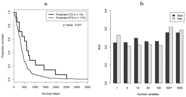
In a), Kaplan–Meier curves comparing overall survival of patients predicted as LTS versus STS for experiment 1. Predictions were made on DNA methylation data using the NBC algorithm with 2 years as the survival threshold. In b), AUC values are plotted against the number of top-ranked genes included in models; more genes equated to better performance

Models based on somatic mutation data performed relatively poorly. The top-ranked genes (e.g., PRAME, FRAP1, GRM1, PTCH1, EPHA3) were mutated differentially between LTS and STS; however, because many of the genes were mutated infrequently (often only two to three times across the population), the models failed to generalise.

When C5.0 and SVM models were constructed using data from all categories, the performance was better than for individual data categories in isolation, a pattern that suggests these algorithms may be useful for modelling inter-category relationships. Among the variables ranked most highly in feature selection was age at diagnosis and treatment variables, a pattern that suggests that much of the discriminatory power of these models was driven by previously known prognosis variables for GBM.

4.2 Experiment 2: 2-year survival threshold, prior knowledge variable selection

The second experiment was performed using prior knowledge variables and 2 year as the survival threshold. Table 4 lists results for this experiment. As illustrated in Figure 3, two results that were statistically significant according to the log-rank test were:

Table 4.

Cross-validation results for experiment 2. AUC values above 0.60 and log-rank p-values below 0.05 are highlighted with an asterisk. Missing log-rank values could not be calculated because all predictions were for the same class

		Clinical	Treatments	Histology	DNA Methylation	Somatic Mutations	DNA Copy Number	mRNA Expression	miRNA Expression	All Data
AUC	C5.0	0.50	0.50	0.50	0.50	0.50	0.50	0.50	0.50	0.56
	NBC	0.68*	0.60	0.43	0.57	0.52	0.50	0.54	0.46	0.57
	SVM	0.51	0.50	0.46	0.51	0.35	0.43	0.46	0.45	0.42
Log-rank	C5.0	–	–	–	–	–	–	–	–	0.03*
	NBC	0.065	–	–	0.3	0.0048*	0.42	0.006*	0.17	0.6
	SVM	–	–	–	0.92	0.63	–	–	–	–

Figure 3.

Kaplan-Meier curves comparing overall survival of patients predicted as LTS versus STS for SVM models trained on DNA methylation data. SVM-RFE was used for variable selection and 2 years was the survival threshold

• NBC models trained on TP53 and IDH1 somatic mutations (p = 0.0048)

• NBC models trained on mRNA expression data (p = 0.006).

Interestingly, even though the NBC somatic-mutation models attained significance via the log-rank test, the AUC value (0.52) was only slightly higher than what would be expected by random chance (0.50). This result demonstrates a key observation that arose in this study: no single metric is suitable in isolation to quantify classification performance. In this case, the log-rank statistic highlighted a small subset of patients who had significantly longer survival than the remaining patients; indeed, these patients were enriched for IDH1 mutations, which have been suggested to lengthen GBM survival in the small subset of patients who acquire them (Bujko et al., 2010). Of the LTS-predicted patients, two survived 603 and 691 days – values that were only slightly less than the survival threshold. Thus, while these patients were misclassified, the NBC algorithm still identified a patient subset with likely clinical relevance. The fact that mRNA-expression models performed well was unsurprising, given that Colman et al. (2010) had derived the gene set from multiple, independent data sources and had used 2-year survival as their threshold. That their gene set also generalised to TCGA at a significant level lends further credence to the clinical relevance of that gene set.

However, it was somewhat surprising that no model attained significance for any other data category. Even clinical models, which accounted for age and KPS – two well-known GBM prognostic variables – failed to reach significance. Again in this case, it is important to acknowledge that no single performance metric is adequate. Even though the log-rank statistic was not significant for the NBC models, the AUC value was relatively high (0.68, see ROC curve in Figure 4(a)). A look at the Kaplan-Meier survival curves (see Fig. 4(b)) reveals that LTS-predicted patients had longer overall survival but that the two curves intersect at one point. This intersection was due to a single patient (the patient who survived the longest in this cohort) being misclassified. Thus, in this case, the importance of considering both metrics and visually inspecting the associated graphs is demonstrated.

Figure 4.

In a), AUC for NBC models trained on clinical variables that have been reported in the literature to have prognostic relevance for GBM. In b), the associated Kaplan-Meier plot

4.3 Experiment 3: Empirical survival thresholds

In the third experiment, the survival threshold was determined using the empirical method. Across all cross-validation folds, the selected thresholds varied between 69.5 days and 147 days (see Fig. 5(a)). Thus, in contrast to the previous experiments, the great majority of patients were considered LTS in this experiment.

Figure 5.

Overall survival for patients receiving radiation treatment versus patients not receiving radiation treatment

In examining the classification models that were used to determine the thresholds, it became apparent that radiation treatment was an extremely strong predictor of survival status at the selected thresholds. In cross validation, predictions based on treatment data (which include radiation) performed exceptionally well by all measures. Patients who received no radiation treatment survived drastically shorter than patients who received radiation treatment (see Fig. 5(b)). Such an observation is not new – multiple studies had previously observed this relationship (Davis et al., 1949; Rich et al., 2005; Ruano et al., 2009). However, this experiment suggests that radiation treatment is more highly prognostic than most (or all) other predictor variables. This finding was observable particularly when the survival threshold was determined empirically and suggests that patients who receive no radiation treatment can typically expect a short survival, regardless of other clinical or biomolecular factors. However, this strong association likely represented a confounding effect. Failure to receive radiation may be a surrogate indicator of a patient’s age or overall health status. For example, some patients may feel they are too old or frail to receive radiation treatment. Indeed, in the TCGA data, patients who received no radiation treatment were considerably older and had lower overall KPS than patients who received radiation. Only a slight trend existed between patient survival and the number of days before radiation treatment started; this suggests that non-radiation-treated patients did not simply delay treatment and then decease prematurely as a consequence.

4.4 Experiment 4: Median survival threshold, radiation-treated patients only

Because radiation- and drug-treatment variables appeared to convey a confounding effect when all data were combined in Experiments 1, 2 and 3, these variables were excluded from Experiment 4. Any patient who did not receive radiation treatment was also excluded, after which 261 patients remained. Additionally, for simplicity and to avoid any effects of class imbalance, the median survival (423 days) was the threshold used in experiment 4.

Table 5 lists results for this experiment. Once again, clinical models (primarily based on age) and DNA methylation models performed relatively well. All Data models also performed fairly well, but the remaining data categories performed moderately or poorly. It should also be noted that in some cases, a statistically significant p-value was attained when the AUC value was quite low (e.g., SVM models of histology and miRNA expression); in these cases, visual inspection of the Kaplan-Meier plots revealed that the curves were separate from each other but in the wrong direction.

Table 5.

Cross-validation results for experiment 4. AUC values above 0.60 and log-rank p-values below 0.05 are highlighted with an asterisk

		Clinical	Treatments	Histology	DNA Methylation	Somatic Mutations	DNA Copy Number	mRNA Expression	miRNA Expression	All Data
AUC	C5.0	0.54	N/A	0.50	0.50	0.44	0.49	0.49	0.49	0.52
	NBC	0.61*	N/A	0.49	0.60	0.42	0.49	0.52	0.51	0.58
	SVM	0.55	N/A	0.40	0.59	0.50	0.48	0.50	0.42	0.56
Log-rank	C5.0 NBC	0.0027*	N/A	0.83 0.73	0.96	0.23	0.32	0.93	0.71	0.099
	SVM	9.5e-06*	N/A	0.023*	0.0031*	0.53	0.36	0.58	0.36	0.012*
		0.0022*			0.054	0.49	0.95	0.23	0.029*	0.011*

5 Discussion

Until recent years, GBM prognosis studies have been limited to small-scale efforts in which one or a few variables were evaluated at a time. Although some factors may determine a GBM patient’s fate in isolation, it is likely that in most cases multiple factors work in concert to influence tumour aggressiveness and ultimately survival. Biomolecular aberrations are at the root of tumour initiation and progression (Ohgaki et al., 2004), but no prognosis model based on biomolecular data is in widespread use among clinicians who treat GBM patients (Colman et al., 2010). Because technological advances are making it possible to examine cancer cells with increasing granularity and at decreasing costs, an important opportunity is arising for researchers to develop multivariate models that help clinicians and patients better understand their survival expectations.

The goal of this study was to assess how well multivariate algorithms could account for combinations of candidate prognosis variables by differentiating between GBM patients who survived a relatively long or short time after diagnosis. Several algorithms were applied to eight categories of GBM patient data and predictive performance was evaluated in a cross-validated design. In several cases, the algorithms were successful at identifying subsets of patients who experienced significantly longer or shorter survival. Across the experiments, the data categories that appeared to contain most prognostic relevance were treatments, clinical and DNA methylation. The treatment data in this study appeared to be confounded by the variability in treatment approaches administered, so inferences about the efficacy of individual treatments are unwarranted; however, the methodologies applied here may be useful in other studies where treatments are more standardised. The consistency with which clinical and DNA methylation data performed across the various experiments suggests that these two categories hold particular promise for informing GBM prognoses, are robust to changes in survival threshold and may hold prognostic relevance independent of treatment-related effects.

A desirable outcome of this study might have been that one classification algorithm performed well in all cases and thus might be favoured for further development of GBM prognosis models. However, in this study, classification performance varied substantially across algorithms. NBC performed relatively well in many cases, particularly when the number of predictor variables was small. When all data were combined, C5.0 Decision Trees and SVM often performed better than NBC and better than when individual data categories were evaluated, perhaps an indication that these algorithms are relatively well suited to modelling cross-category interactions in high-dimensional data sets.

Even though several of our classification models had limited success in predicting survival status, it should not be inferred that effective prognosis models are impossible – or even unlikely – to be developed for any given data category. Such inferences could become Type II errors as methods of developing such models are refined. We applied commonly used, general-purpose algorithms to the GBM data to gain a sense for the predictive performance that can be attained. Other algorithms or different methods of preprocessing the data may prove valuable in future studies.

Because various types of molecular aberrations can influence tumour growth, a key goal of the TCGA Consortium is to facilitate development of methods that integrate data across modalities. This study has demonstrated one approach for performing integrative analyses: combining all data into an aggregate data set, thus allowing multivariate algorithms to model intercategory relationships at a granular level. In some cases, these models performed better than the single-category models, an indication that aggregating data may indeed be useful. Other approaches – for example, ensemble-learning approaches – may also be useful. It is likely that researchers increasingly will apply such integrative methods as multimodal data sets become more common (Xu et al., 2011).

5.1 Lessons learned

Standardised protocols do not yet exist for performing experiments such as those in this study. General guidelines must be followed to ensure statistical and methodological rigor; however, many seemingly minor decisions – each of which could impact the results – must be made. In this study, an attempt has been made to default such decisions toward the simplest approach, which may not be optimal in every case. This section elucidates a few such methodological factors that must be considered in performing such a study as well as issues to be considered in interpreting such a study. It is hoped that these lessons will serve as a reference point for future classification studies in TCGA (and elsewhere). GBM was the first cancer type with a substantial amount of data in TCGA, but the US government is investing an additional $275 million so that TCGA will eventually cover more than 20 cancer types (Consortium, n.d.).

The choice of data-summarisation techniques requires careful consideration. For example, treatment data were transformed into binary values in this study to maintain simplicity, even though patients who receive multiple doses of a given drug may gain more benefit than patients who receive a single dose. Additionally, all biomolecular data were summarised according to higher level functional categories. For example, somatic-mutation, DNA methylation and mRNA expression data were summarised at the gene level. Although summarising raw data may sometimes reduce signal, summarisation methods enable easier interpretation, reduce computational demands and may represent underlying biological mechanisms better than raw data.

Ideally, retrospective data sets like TCGA would contain data only for patients who had been treated uniformly with one or a few specific treatments, as in clinical trials. Such a design would enable assessments of the effectiveness of specific treatments and of cofactors that may influence treatment responses. However, until recently, the GBM standard of care has not included specific drug treatments, so a wide variety of drug treatments and regimens were administered. Various tactics could be employed to account for this heterogeneity, such as:

• limiting analyses to patients who received specific treatments

• treating treatments as stratification variables in multivariate survival analyses.

We chose the former approach in Experiment 4 because of its simplicity; but one drawback of this approach is that it reduces sample sizes and thus statistical power.

Transforming time-to-event data into a binary value (e.g., STS, LTS) can result in a loss of information (Dupuy and Simon, 2007); however, to be consistent with prior studies (Colman et al., 2010; Liang et al., 2005; Nutt et al., 2003), we discretised survival. This approach can introduce bias if the two groups have different censorship structures (Dupuy and Simon, 2007); however, we avoided such a bias by excluding patients who were still alive (n = 74) when the analysis was performed. Although this exclusion affected sample size only moderately in this study, such an approach may not be acceptable when studying other cancer types or which survival is generally longer. The Cox proportional hazards model (Cox, 1972), which retains survival as a continuous variable and accounts for censorship structure may be more suitable for general application. Traditional Cox models were not designed for data sets that contain thousands of variables and thus may not perform well in this setting; however, relevant variations on this model may be useful (Liu and Jiang, 2009). Additionally, physicians may prefer discrete rather than continuous risk predictions – for example, they may prefer to tell a patient that they have a “90% chance of surviving 2 years” than to tell the patient that their “estimated survival time is 750 days.”

Two variables that are not recorded in TCGA but that may have offered valuable insights are:

1. tissue anatomic site

2. year of diagnosis

In the Lamborn et al. (2004) study, tissue anatomic site showed promise as a prognostic factor; it is plausible that GBM tumours differ in their aggressiveness, operability and in the effects they have on cognitive function, depending on the location of the brain from which the tumour arises. Evaluating the relationship between year of diagnosis and patient survival may offer insights into confounding effects that can result from changes in treatments, surgical techniques, methods of tumour-sample preservation, etc. that occur across a span of years or decades.

TCGA data are provided by several research centres throughout the United States. While special efforts are being made to ensure consistency in specimen handling, tumour-sample quality and clinical data definitions, the TCGA data by nature are heterogeneous and likely to contain noise that could impact predictive performance. Acknowledging this limitation, an added measure of confidence can be placed on models that do perform well on this data set.

6 Conclusion

The aggressive nature of GBM leaves clinicians with a relatively short time span to determine optimal treatments for each patient. Although radiation treatment, surgical resection and temozolomide treatment have shown promise for lengthening GBM survival times, few patients survive longer than 5 years after diagnosis. A better understanding of factors that are associated with GBM survival – and thus that may indicate a lack of response to standard treatments – could help clinicians prioritise patients for clinical trials and help patients make decisions about entering such trials. An increased understanding of the biological mechanisms that drive tumour aggressiveness – and that may differentiate the most (or least) lethal tumours from the remaining tumours – may also lead researchers to molecularly targeted treatments that improve patient outcomes.

Even though a long road may still lie ahead for researchers working to eradicate devastating diseases like GBM, data-mining techniques such as those presented in this study promise to guide researchers in their efforts to improve outcomes and explain the biological underpinnings of disease.

Biographies

Stephen R. Piccolo received his PhD in Biomedical Informatics in 2011 from the University of Utah, USA. Currently, he is a Post-doctoral Researcher at the University of Utah. His research interests include analysis of high-throughput genomics data, development of software tools to analyse such data and application of such tools to cancer biology and treatment.

Lewis J. Frey received his PhD in computer science from Vanderbilt University, USA. Currently, he is an Assistant Professor of Biomedical Informatics at the University of Utah, USA and a member of the Huntsman Cancer Institute. His research interests include data integration and analysis of heterogeneous clinical and bioinformatics data sets for the purpose of knowledge discovery. His work on data integration and analysis have been applied to interoperable biomedical informatics systems that have wide applicability across medicine in such areas as cancer, paediatric care and newborn screening.

References

- Breiman L, Friedman J, Stone CJ, Olshen RA. Classification and Regression Trees. Chapman and Hall/CRC; Boca Raton: 1984. [Google Scholar]
- Bujko M, Kober P, Matyja E, Nauman P, Dyttus-Cebulok K, Czeremszynska B, Bonicki W, Siedlecki JA. Prognostic value of IDH1 mutations identified with PCR-RFLP assay in glioblastoma patients. Molecular Diagnosis & Therapy. 2010;14(3):163–169. doi: 10.1007/BF03256369. [DOI] [PubMed] [Google Scholar]
- Burger PC, Green SB. Patient age, histologic features and length of survival in patients with glioblastoma multiforme. Cancer. 1987;59(9):1617–1625. doi: 10.1002/1097-0142(19870501)59:9<1617::aid-cncr2820590916>3.0.co;2-x. [DOI] [PubMed] [Google Scholar]
- Burton EC, Lamborn KR, Feuerstein BG, Prados M, Scott J, Forsyth P, Passe S, Jenkins RB, Aldape KD. Genetic aberrations defined by comparative genomic hybridization distinguish long-term from typical survivors of glioblastoma. Cancer Res. 2002;62(21):6205–6210. [PubMed] [Google Scholar]
- Cadieux B, Ching T, VandenBerg SR, Costello JF. Genome-wide hypomethylation in human glioblastomas associated with specific copy number alteration, methylenetetrahydrofolate reductase allele status and increased proliferation. Cancer Res. 2006;66(17):8469–8476. doi: 10.1158/0008-5472.CAN-06-1547. [DOI] [PubMed] [Google Scholar]
- Chang C, Lin C. LIBSVM: A Library For Support Vector Machines. [accessed January 31, 2011];Obtained through the Internet. 2001 http://www.csie.ntu.edu.tw/~cjlin/libsvm.
- Colman H, Zhang L, Sulman EP, McDonald JM, Shooshtari NL, Rivera A, Popoff S, Nutt CL, Louis DN, Cairncross JG, Gilbert MR, Phillips HS, Mehta MP, Chakravarti A, Pelloski CE, Bhat K, Feuerstein BG, Jenkins RB, Aldape K. A multigene predictor of outcome in glioblastoma. Neuro Oncol. 2010;12(1):49–57. doi: 10.1093/neuonc/nop007. [DOI] [PMC free article] [PubMed] [Google Scholar]
- Cox DR. Regression models and life-tables. Journal of the Royal Statistical Society. Series B (Methodological) 1972;34(2):187–220. [Google Scholar]
- Davis L, Martin J, Goldstein SL, Ashkenazy M. A study of 211 patients with verified glioblastoma multiforme. J Neurosurg. 1949;6(1):33–44. doi: 10.3171/jns.1949.6.1.0033. [DOI] [PubMed] [Google Scholar]
- Domingos P, Pazzani M. On the optimality of the simple bayesian classifier under zero-one loss. Mach Learn. 1997;29(2):103–130. [Google Scholar]
- Dupuy A, Simon RM. Critical review of published microarray studies for cancer outcome and guidelines on statistical analysis and reporting. J Natl Cancer Inst. 2007;99(2):147–57. doi: 10.1093/jnci/djk018. [DOI] [PubMed] [Google Scholar]
- Edgerton ME, Fisher DH, Tang L, Frey LJ, Chen Z. Data mining for gene networks relevant to poor prognosis in lung cancer via backward-chaining rule induction. Cancer Inform. 2007;3:93–114. [PMC free article] [PubMed] [Google Scholar]
- Fearon ER, Vogelstein B. A genetic model for colorectal tumorigenesis. Cell. 1990;61(5):759–67. doi: 10.1016/0092-8674(90)90186-i. [DOI] [PubMed] [Google Scholar]
- Fujita PA, Rhead B, Zweig AS, Hinrichs AS, Karolchik D, Cline MS, Goldman M, Barber GP, Clawson H, Coelho A, Diekhans M, Dreszer TR, Giardine BM, Harte Ra, Hillman-Jackson J, Hsu F, Kirkup V, Kuhn RM, Learned K, Li CH, Meyer LR, Pohl A, Raney BJ, Rosenbloom KR, Smith KE, Haussler D, Kent WJ. The UCSC genome browser database: Update 2011. Nucleic Acids Res. 2011;39:D876–D882. doi: 10.1093/nar/gkq963. [DOI] [PMC free article] [PubMed] [Google Scholar]
- Guyon I, Weston J, Barnhill S, Vapnik V. Gene selection for cancer classification using support vector machines. Mach Learn. 2002;46(1):389–422. [Google Scholar]
- Hall M, Frank E, Holmes G, Pfahringer B, Reutemann P, Witten IH. The WEKA data mining software. ACM SIGKDD Explorations Newsletter. 2009;11(1):10. [Google Scholar]
- Houillier C, Lejeune J, Benouaich-Amiel A, Laigle-Donadey F, Criniere E, Mokhtari K, Thillet J, Delattre JY, Hoang-Xuan K, Sanson M. Prognostic impact of molecular markers in a series of 220 primary glioblastomas. Cancer. 2006;106(10):2218–2223. doi: 10.1002/cncr.21819. [DOI] [PubMed] [Google Scholar]
- Issa JJ. Methylation and prognosis: of molecular clocks and hypermethylator phenotypes. Clin Cancer Res. 2003;9(8):2879–2881. [PubMed] [Google Scholar]
- Jemal A, Siegel R, Ward E, Hao Y, Xu J, Thun MJ. Cancer statistics, 2009. CA Cancer J Clin. 2009;59(4):225–249. doi: 10.3322/caac.20006. [DOI] [PubMed] [Google Scholar]
- Kaplan EL, Meier P. Nonparametric estimation from incomplete observtions. J Am Stat Assoc. 1958;53(282):457–481. [Google Scholar]
- Krex D, Klink B, Hartmann C, von Deimling A, Pietsch T, Simon M, Sabel M, Steinbach JP, Heese O, Reifenberger G, Weller M, Schackert G Network ftGG. Long-term survival with glioblastoma multiforme. Brain. 2007;130(10):2596–2606. doi: 10.1093/brain/awm204. [DOI] [PubMed] [Google Scholar]
- Lacroix M, Abi-Said D, Fourney DR, Gokaslan ZL, Shi W, DeMonte F, Lang FF, McCutcheon IE, Hassenbusch SJ, Holland E, Hess K, Michael C, Miller D, Sawaya R. A multivariate analysis of 416 patients with glioblastoma multiforme: Prognosis, extent of resection and survival. J Neurosurg. 2001;95(2):190–198. doi: 10.3171/jns.2001.95.2.0190. [DOI] [PubMed] [Google Scholar]
- Lamborn KR, Chang SM, Prados MD. Prognostic factors for survival of patients with glioblastoma: Recursive partitioning analysis. Neuro Oncol. 2004;6(3):227–235. doi: 10.1215/S1152851703000620. [DOI] [PMC free article] [PubMed] [Google Scholar]
- Langley P, Iba W, Thompson K. An analysis of bayesian classifiers. Proceedings of the Tenth National Conference on Artificial Intelligence,; San Jose. 1992. [Google Scholar]
- Liang Y, Diehn M, Watson N, Bollen AW, Aldape KD, Nicholas MK, Lamborn KR, Berger MS, Botstein D, Brown PO, Israel MA. Gene expression profiling reveals molecularly and clinically distinct subtypes of glioblastoma multiforme. Proc Natl Acad Sci U S A. 2005;102(16):5814–5819. doi: 10.1073/pnas.0402870102. [DOI] [PMC free article] [PubMed] [Google Scholar]
- Liu Z, Jiang F. Gene identification and survival prediction with lp cox regression and novel similarity measure. Int J Data Min Bioinform. 2009;3(4):398–408. doi: 10.1504/ijdmb.2009.029203. [DOI] [PubMed] [Google Scholar]
- Mantel N. Evaluation of survival data and two new rank order statistics arising in its consideration. Cancer Chemother Rep. 1966;50(3):163–170. [PubMed] [Google Scholar]
- Nigro JM, Misra A, Zhang L, Smirnov I, Colman H, Griffin C, Ozburn N, Chen M, Pan E, Koul D, Yung WKA, Feuerstein BG, Aldape KD. Integrated array-comparative genomic hybridization and expression array profiles identify clinically relevant molecular subtypes of glioblastoma. Cancer Res. 2005;65(5):1678–86. doi: 10.1158/0008-5472.CAN-04-2921. [DOI] [PubMed] [Google Scholar]
- Noble WS. What is a support vector machine? Nat Biotechnol. 2006;24(12):1565–1567. doi: 10.1038/nbt1206-1565. [DOI] [PubMed] [Google Scholar]
- Nutt CL, Mani DR, Betensky RA, Tamayo P, Cairncross JG, Ladd C, Pohl U, Hartmann C, McLaughlin ME, Batchelor TT, Black PM, von Deimling A, Pomeroy SL, Golub TR, Louis DN. Gene expression-based classification of malignant gliomas correlates better with survival than histological classification. Cancer Res. 2003;63(7):1602–1607. [PubMed] [Google Scholar]
- Ohgaki H, Kleihues P. Genetic pathways to primary and secondary glioblastoma. Am J Pathol. 2007;170(5):1445–1453. doi: 10.2353/ajpath.2007.070011. [DOI] [PMC free article] [PubMed] [Google Scholar]
- Ohgaki H, Dessen P, Jourde B, Horstmann S, Nishikawa T, Di Patre PL, Burkhard C, Schiiler D, Probst-Hensch NM, Maiorka PCC, Baeza N, Pisani P, Yonekawa Y, Yasargil GG, Lutolf UM, Kleihues P. Genetic pathways to glioblastoma: a population-based study. Cancer Res. 2004;64(19):6892–6899. doi: 10.1158/0008-5472.CAN-04-1337. [DOI] [PubMed] [Google Scholar]
- Piccolo SR. Dissertation. University of Utah, Utah; United States: 2011. Informatics Framework for Evaluating Multivariate Prognosis Models: Application to Human Glioblastoma Multiforme. [Google Scholar]
- Piccolo SR, Frey LJ. ML-Flex: A Flexible Toolbox for Performing Classification Analyses In Parallel. Journal of Machine Learning Research. 2012;13:555–559. [Google Scholar]
- Quinlan JR. C4-5: Programs for Machine Learning. Morgan Kaufmann; San Mateo: 1993. [Google Scholar]
- R: A language and environment for statistical computing. Vienna, Austria: R Foundation for Statistical Computing; 2008. Version 2.11.0. [Google Scholar]
- Rich JN, Hans C, Jones B, Iversen ES, McLendon RE, Rasheed AK, Dobra A, Dressman HK, Bigner DD, Nevins JR, West M. Gene expression profiling and genetic markers in glioblastoma survival. Cancer Res. 2005;65(10):4051–4058. doi: 10.1158/0008-5472.CAN-04-3936. [DOI] [PubMed] [Google Scholar]
- Ruano Y, Ribalta T, de Lope AR, Campos-Martin Y, Fiano C, Perez-Magan E, Hernandez-Moneo J, Mollejo M, Melendez B. Worse outcome in primary glioblastoma multiforme with concurrent epidermal growth factor receptor and p53 alteration. Am J Clin Pathol. 2009;131(2):257–263. doi: 10.1309/AJCP64YBDVCTIRWV. [DOI] [PubMed] [Google Scholar]
- Stupp R, Mason WP, van den Bent MJ, Weller M, Fisher B, Taphoorn MJB, Belanger K, Brandes AA, Marosi C, Bogdahn U, Curschmann J, Janzer RC, Ludwin SK, Gorlia T, Allgeier A, Lacombe D, Cairncross JG, Eisenhauer E, Mirimanoff RO. Radiotherapy plus concomitant and adjuvant temozolomide for glioblastoma. N Engl J Med. 2005;352(10):987–996. doi: 10.1056/NEJMoa043330. [DOI] [PubMed] [Google Scholar]
- The Cancer Genome Atlas Research Consortium. The Cancer Genome Atlas Project to Map 20 Tumor Types. [accessed October 25, 2010];Obtained through the Internet. http://tcga.cancer.gov/wwd/program.
- The Cancer Genome Atlas Research Network . Comprehensive genomic characterization defines human glioblastoma genes and core pathways. Nature. 2008;455(7216):1061–1068. doi: 10.1038/nature07385. [DOI] [PMC free article] [PubMed] [Google Scholar]
- Therneau T, Lumley T. Survival: Survival Analysis, Including Penalised Likelihood. [accessed December 29, 2010];Obtained through the Internet. 2009 http://cran.r-project.org/package=survival.
- Vapnik VN. Statistical Learning Theory. Wiley; New York: 1998. [Google Scholar]
- Xu Q, Xue H, Yang Q. Multi-platform gene-expression mining and marker gene analysis. Int J Data Min Bioinform. 2011;5(5):485–503. doi: 10.1504/ijdmb.2011.043030. [DOI] [PubMed] [Google Scholar]