Improving brain-machine interface performance by decoding intended future movements

Abstract

Objective

A brain-machine interface (BMI) records neural signals in real time from a subject’s brain, interprets them as motor commands, and reroutes them to a device such as a robotic arm, so as to restore lost motor function. Our objective here is to improve BMI performance by minimizing the deleterious effects of delay in the BMI control loop. We mitigate the effects of delay by decoding the subject’s intended movements a short time lead in the future.

Approach

We use the decoded, intended future movements of the subject as the control signal that drives the movement of our BMI. This should allow the user’s intended trajectory to be implemented more quickly by the BMI, reducing the amount of delay in the system. In our experiment, a monkey (Macaca mulatta) uses a future prediction BMI to control a simulated arm to hit targets on a screen.

Main Results

Results from experiments with BMIs possessing different system delays (100, 200, and 300 milliseconds) show that the monkey can make significantly straighter, faster, and smoother movements when the decoder predicts the user’s future intent. We also characterize how BMI performance changes as a function of delay, and explore offline how the accuracy of future prediction decoders varies at different time leads.

Significance

This study is the first to characterize the effects of control delays in a BMI and to show that decoding the user’s future intent can compensate for the negative effect of control delay on BMI performance.

1. Introduction

Brain-machine interfaces (BMI) seek to restore a paralyzed patient’s lost motor function by recording movement commands directly from the patient’s brain and rerouting them to an external device, such as a computer cursor or a prosthetic arm. While there are many types of BMIs, our focus is on BMIs that use intra-cortical electrodes to record single and multi-unit activity from neurons in the primary motor cortex (MI) enabling the user to make continuous reaching movements. Several research groups in the past decade have demonstrated the successful use of this kind of BMI by both non-human primates and human subjects (Kennedy et al 2000, Taylor et al 2002, Serruya et al 2002, Carmena et al 2003, Velliste et al 2008, Kim et al 2008, Suminski et al 2010, Kim et al 2011, Chadwick et al 2011). However, the performance of BMI systems is still far poorer than that of a healthy subject’s own arm, and many aspects remain to be improved. In this paper, we focus on the negative effect of control loop delays on BMI performance and propose a new approach to decoding that can achieve faster response times for BMIs.

A key element of any BMI is the “decoder” that translates neural activity into a motor command. In most cases, it is an estimate of the user’s desired arm state (or cursor state, in the case of controlling a computer cursor) at the present time. Typically, the user’s desired hand position or hand velocity is decoded, although other variables such as desired joint torques or muscle activations are possible when controlling a limb. There are two dominant, clinically relevant approaches to training a decoder that can predict the user’s desired arm state (DAS) from a recent history of the user’s neural activity: (1) a visual observation paradigm, where the subject watches an arm or a cursor make reaching movements while the decoder is trained to use the subject’s neural activity to predict the state of the arm being observed by the subject (Tkach et al 2007, Kim et al 2008, Suminski et al 2010), or (2) an adaptive decoding paradigm, where the subject uses the BMI in real time to attempt to complete a task while the decoder is trained to use the subject’s neural activity to predict what is assumed to be the user’s DAS during the task (Taylor et al 2002, Gage et al 2005, Orsborn et al 2012). In the visual observation paradigm, a recent history of the subject’s neural activity is associated with the state of the observed limb at the present time. Similarly, in the adaptive decoding paradigm, a recent history of the subject’s neural activity is associated with what is believed to be the user’s DAS at the present moment. These two approaches are not mutually exclusive, and both approaches, used alone or in combination, yield a decoder that is capable of predicting the user’s DAS at the current time t while making use of the user’s neural history up to time t.

In the case where a BMI enables near instantaneous control of a device, such as the state of a computer cursor on a screen, the user’s DAS can be implemented as soon as it is decoded. In this case, there is minimal lag between the user’s DAS and the state of the cursor. However, when controlling a mechanical device such as a prosthetic limb, instantaneous control of its state is not possible. In the BMI literature, robotic limbs are typically controlled with a proportional-derivative controller that selects the appropriate joint torques required to bring the limb to a desired velocity or position. These joint torques take time to be implemented by the motors in the arm and to overcome the inertia of the limb so as to move it to a desired velocity or position. Since decoders typically identify the subject’s DAS at the present moment, any extra time needed to effect a change in the limb’s state introduces a lag between the subject’s DAS and the actual state of the arm, which in some cases can be substantial. Additional delay is sometimes added when the user’s DAS or neural activity is smoothed with a low-pass filter; while this strategy reduces noise in the command signal, it adds more temporal lag.

Several examples of these kinds of control delay can be found in the BMI literature. In one early study, a monkey controlled a BMI with a robotic arm in the control loop that added 60–90 ms of delay (Carmena et al 2003). In another landmark study, where monkeys used a BMI to control a robotic arm in order to complete a self-feeding task, at least two sources of delay were present: delay from control of the robotic arm, and delay from smoothing that the authors imposed on the neural activity in order to reduce high frequency noise in the decoded velocity (Velliste et al 2008). The total estimated delay in this study was 150 ms. While these studies demonstrate the ability to successfully control a robotic device with a BMI, such control delays are likely to have a significant negative effect on performance. At the very least, control delay increases the initial reaction time of the reach by the amount of control delay added. In addition, delay in the control loop slows down any corrections that might need to be made during the reach, reducing accuracy. Control delay also lengthens the amount of time between the user’s command signal and the sensory feedback about its consequences, potentially resulting in oscillations, and often requiring the user to rely more on a potentially inaccurate feed-forward model of the arm.

Research on the effects of delay in non-human primates and humans confirms the deleterious effects of delay on reaching in a variety of tasks. In a series of studies on a manual tracking task, it was shown that delayed visual feedback degraded performance and decreased the frequency of corrective movements, since subjects had to wait longer for feedback about the state of their arm (Miall et al 1985, Foulkes and Miall 2000, Miall and Jackson 2006). In this work, some adaptation occurred, but performance never returned to baseline. Another study found that human subjects making reaching movements on a touchpad when visual feedback was delayed by 200 ms were slower and less accurate (Shimada et al 2004). Finally, in a study on lag in human computer interaction, MacKenzie and Ware (1993) found that delay added between the user’s movement of a mouse and the corresponding visual feedback on the screen decreased performance on a Fitts’ law clicking task. At 225 ms, the largest delay tested, the movement time was increased by half and the error rate doubled. Since BMI users have less accurate control over their neural activity than healthy subjects have over their own arm, we might expect delay to be even more deleterious in the BMI setting.

In one recent BMI study, the authors measured online BMI performance as a function of their Kalman filter decoder’s bin size, which determined the amount of neural history used in the decoder in addition to the rate at which the decoder updated the cursor’s position (Cunningham et al 2011). The authors found that smaller bin sizes, which used less neural history but caused the decoder to update more quickly, increased BMI performance. This result confirms the idea that reducing the latency in BMI control loops should make BMIs significantly easier to control.

In addition to decreasing the time delay between discrete decoder updates, one approach to decreasing control delays in BMIs could be to train the BMI’s decoder to predict the user’s DAS a short time into the future instead of in the present moment. Because of neural conduction delays and the time it takes for muscles to effect a change in the state of a subject’s limb, the activity of MI neurons contains information about not only the current state of the user’s limb, but also its future state. Two studies that examined the time delay between neural activity in MI and the hand velocity of the subject found that neural activity led movement by about 75 to 100 ms, though there was considerable spread around these means (Paninski et al 2004, Schwartz et al 2004). Another study that examined this time lead when subjects both made and observed movements found mean time leads of 64.6 ± 12.8 and 12.8 ± 22.5 ms, respectively (Tkach et al 2007). By making use of this neural activity that naturally leads movement, “future prediction” decoders may be able to accurately predict the user’s future intent. To be clear, in using the phrase “future prediction” in this paper we are not claiming that the motor cortex itself predicts the future state of the user’s arm in an explicit way. Instead, we believe that feedforward delays in moving a musculoskeletal limb necessarily cause motor cortical activity to lead movement, and that this activity may be able to be used to predict the user’s future intent.

A future prediction approach, if successful, should improve the response time of the BMI system relative to a present prediction strategy. If there is very little delay in implementing the user’s DAS once it has been decoded (e.g., instantaneous control of a computer cursor), then the response time of the BMI could be even faster than the response time of the user’s own arm during natural movement. If there is some delay in the BMI system, but the amount of delay is small enough, predicting into the future at a time lead equal to the control delay should allow the BMI to reach a response time approximately equal to that seen during natural movement. For example, if at the current time the decoder determines that the user would like his or her arm to be at a given state 100 ms in the future, then the BMI will have 100 ms to move the arm into alignment with that state in order to be on time with the user’s intention.

Preliminary work suggested that future prediction improves BMI performance (Willett et al 2012). In this paper, we expanded on that work and tested several hypotheses related to future prediction decoding and delays in BMIs. First, we tested the hypothesis that a neural decoder can successfully predict a subject’s intended hand position a short time in the future. We did so by testing offline the ability of neural decoders to reconstruct reaching movements visually observed by two rhesus macaques at varying future prediction time leads. Second, we also tested the hypothesis that using a future prediction decoder in a BMI with control delays will improve online performance by improving the response time of the BMI. We examined performance data from one rhesus macaque that used BMIs with different control delays and different future prediction time leads. Finally, we tested the hypothesis that delay in BMI control loops will negatively affect performance, and we characterized the performance degradation that occurs when different amounts of delay are added to a BMI.

2. Methods

2.1 Behavioral Task

One adult male rhesus macaque (monkey Mk) was trained to control a simulated arm in a two-dimensional workspace with our BMI that decoded the monkey’s intended hand position based on neural activity in primary motor cortex (MI) from the recent past. Only the hand position of the arm was displayed to the monkey in the form of a cursor. The monkey sat in a primate chair holding his arm still while it was abducted 90 degrees and supported by a two-link robotic exoskeleton (KINARM, BKIN Technologies, Kingston, ON). Direct vision of the monkey’s arm was precluded by a horizontal projection screen, on which the cursor and the targets were projected during the task (figure 1). The task required the monkey to continuously move the cursor (6 mm diameter) to a stationary square target (15 x 15 mm). Each time the monkey hit a target (which only required the cursor to touch the edge of a target with no hold required), a new target appeared immediately in a randomly chosen position among 9 possible locations defined by a 3x3 grid within the workspace (14.2 x 13 cm).

Figure 1.

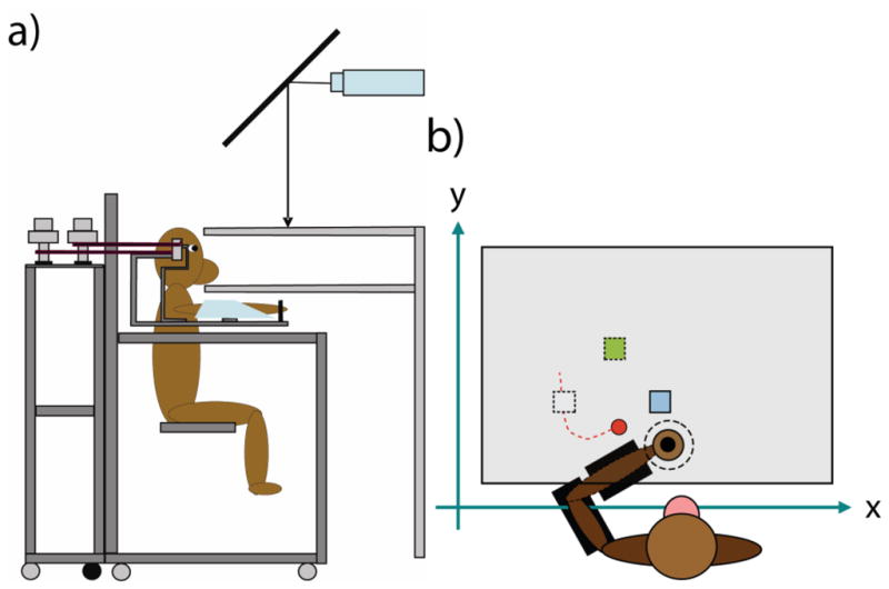
The experimental apparatus and task. (a) The KINARM apparatus and monkey chair in which the monkey sat during each experimental session. The monkey rests his arm in the KINARM exoskeleton, which restricts movements to 2D reaches in the horizontal plane. A screen onto which the game is projected precludes direct vision of the monkey’s own arm. (b) The task during visual observation or brain control. During visual observation, the monkey holds his arm still in the center of the workspace (black circle), observes the cursor (in red) make reaches to targets, and receives a juice reward after a random number of reaches (five to seven). During brain control, the monkey holds his arm still in the center of the workspace and directs the cursor towards targets with neural activity in MI to receive a juice reward. In the figure, the white target represents a recently acquired target, the blue target is the current target, and the green target will appear after the blue target is acquired.

Each experimental session consisted of two conditions: visual observation and brain control. During visual observation, the monkey held his arm still while he observed movements of the cursor hitting targets. These movements were recorded previously while the monkey performed the task with his own arm that was contralateral to the implanted microelectrode array. We trained the neural decoders in our BMI by associating recent spiking activity with the current or future position of the cursor during visual observation. During brain control, the monkey used these neural decoders to control a simulated arm (figure 2), whose hand position was displayed to the monkey as a cursor in the 2D workspace. In order to complete a successful trial and receive a juice reward, the monkey was required to sequentially acquire two to three targets (brain control) or five to nine targets (visual observation). The task proceeded continuously after a reward was administered, with no breaks in between trials or blocks. In either condition, if the monkey moved his arm outside of a 2 cm diameter circle in the center of the KINARM’s workspace, the screen was shut off and the robotic exoskeleton moved his arm back to the center of the workspace. A trial was aborted if any movement between targets took longer than 5 seconds. When this occurred, a new trial began immediately and a new target was presented.

Figure 2.

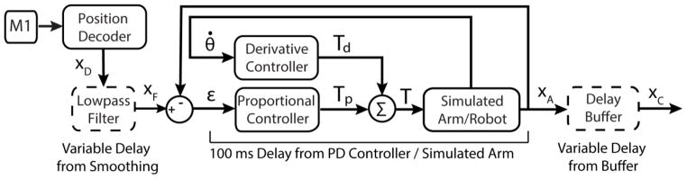
Our BMI uses neural activity recorded from the primary motor cortex to generate an intended hand position in Cartesian space, which the monkey then uses to hit targets. X_D, X_F, X_A, and X_C are two-element column vectors containing the X and Y components of a hand position in Cartesian space, ε is a two-element column vector containing the X and Y components of an error signal, θ̇ is a two-element column vector containing elbow and shoulder joint velocities, and T_p, T_d, and T are two-element column vectors containing joint torque terms. Three sources of delay are illustrated: a low-pass Butterworth filter that smooths the output of the position decoder (X_D), a PD controller that drives the arm towards X_F, and a buffer that delays the display of the simulated arm’s hand position (X_A). In our experiments, we manipulated the amount of delay inserted by the low-pass filter and buffer (illustrated by the dashed outlines). It is important to note that the base level of delay added by our decoder and our electronic equipment is not illustrated, but is present in all online experiments reported (see section 2.2). We estimate this delay to be 80 ms on average.

A different rhesus macaque (monkey B) was trained to perform a similar task with some minor differences. First, the target locations were not fixed to a grid and could appear anywhere within the workspace. Second, the workspace was significantly wider than it was tall (12 x 6 cm). Target size, cursor size, and other relevant parameters of the game remained the same. Data from several sessions of visual observation collected with monkey B were used to confirm the trends seen in the offline decoding results with monkey Mk. No data from online BMI sessions with monkey B are reported in this study.

2.2 Real-Time BMI

Our BMI (figure 2) uses the neural activity of the subject to drive the movement of a two-link simulated arm. This simulated arm captures the dynamics of both the KINARM and the monkey’s arm, as described in Fagg et al. (2009). X_c represents the position of the hand and determines the location of the cursor on the screen. The torques, T, which drive the arm, are generated by a Proportional-Derivative (PD) controller that moves the simulated arm towards X_F, the low-pass filtered estimate of the monkey’s intended hand position. The PD controller causes the simulated arm to lag behind the filtered, decoded position by approximately 100 ms.

The position decoder, implemented as a linear, finite impulse response (FIR) filter, predicts the monkey’s intended hand position, X_D, from the neural data. In our approach, the neural activity is represented as a series of binned spike counts, and the hand position is reconstructed from a linear combination of these spike counts plus a constant offset representing the mean hand position (as in Fagg et. al. 2009). We employ a history of B = 20 bins of Δt = 50 ms each for every neuron, giving the filters access to a total of one second of neural spiking history. Specifically, signal S_k(t) at discrete time bin t (where k is an index representing either X or Y hand position in the present, or at a time lead into the future) is reconstructed as follows:

$$S_k(t)={\sum }_{j=0}^{B-1}{\sum }_{i=0}^{C-1}A(k,j,i)\ast N(i,t-j)+c_k,$$

where i indexes over the C neurons, j indexes over time bins, N(i, t) is the spike count of neuron i over time bin t, A are the coefficients of the filter, and c_k is an offset parameter for signal S_k. The coefficients are solved for analytically with ridge regression (Björck 1996), using 250 seconds of spiking activity and cursor movement data collected during visual observation. Our implementation of ridge regression minimizes the sum of squared errors of prediction plus the sum of squared filter coefficients multiplied by a constant value α. Minimizing the magnitude of the coefficients helps to guard against overfitting. We set α equal to 0.2 times the largest eigenvalue of the firing rate correlation matrix (NN^T), divided by the number samples used to train the decoder.

To obtain a decoder that predicts intended future movement, we solve for the coefficients that best predict the cursor position at some lead time into the future, relative to the one second of spiking history. This requires only a simple alteration of the training data set to pair the neural data with the state of the cursor at a given time lead, τ, into the future. Figure 3 illustrates the difference between this future prediction approach and a present prediction approach.

Figure 3.

Idealized representation of the spiking activity of 5 neurons in MI generated when a subject makes a reach or observes a reach being made by another subject. The neural activity deviates from baseline a short time before the arm begins to move, suggesting that information about the user’s upcoming movement can be decoded before the movement is actually made. Our future prediction decoders are trained to use this information to predict the user’s intended movement a short time lead τ into the future, helping to achieve the fastest possible response time for the BMI.

In some experiments, the decoded position X_D, representing the monkey’s intended hand position in the present or in the future, is filtered using a 6^th order, low-pass Butterworth filter (cutoff frequency = 3.0 Hz or 1.6 Hz), adding an additional delay to the decoded position signal of approximately 100 or 200 ms. Finally, in one online experiment, the appearance of the cursor on the screen is delayed by a constant amount by using a buffer. We call this a “pure” delay and vary it to manipulate the amount of delay in the BMI system.

Finally, it is important to note the amount of latency added by the discrete decoder updates and the electronics used to process the neural data in real-time and to display visual feedback. We estimate this latency to be 80 ms on average. Our decoder updates its estimate of the user’s intended hand position in discrete 50 ms time steps, and can therefore be understood to add an average delay of 25 ms between neural spiking events and when those events can begin to effect a change in the position of the cursor. Our electronics add an average of 55 ms of delay, with ~ 5 ms of delay coming from the signal processing between the microelectrode array and the central computer, and 49 ± 7 ms (SD) of delay coming from the refresh rate of the display and the communication between the display and the central computer.

2.3 Electrophysiology

Each monkey was implanted with a 100 electrode (400 μm interelectrode separation) microelectrode array (Blackrock Microsystems, Inc., Salt Lake City, UT) in MI. The electrodes on each array were 1.0mm (Monkey Mk) or 1.5 mm (Monkey B) in length. The tips of the electrodes were coated with iridium oxide. During the recording session, signals from up to 96 electrodes were amplified (gain of 5000), bandpass filtered between 0.3 Hz and 7.5 kHz, and recorded digitally (14 bit) at 30 kHz per channel using a Cerebus acquisition system (Blackrock Microsystems) as in our previous work (Fagg et al 2009). Single and multiunit spiking events were sorted online and used to train and drive the BMI during the experiments. Waveforms that crossed a user-defined threshold and whose voltage was within a user-defined range at one or more time points were classified as a spiking event for a given neural unit. Thresholds and sorting windows for each neural unit were set by visual inspection at the beginning of the experiment.

For the visual observation datasets used during our offline analyses, we sampled an average of 69.3±3.8 (mean±standard deviation) neural units for monkey Mk and 54.6±17.1 neural units for monkey B. The signal-to-noise ratios (SNRs) of these neural units had an average value of 3.55±1.41 (Monkey Mk) and 4.92±1.52 (Monkey B). SNRs were defined as the difference in mean peak-to-trough voltage of the waveforms divided by the mean standard deviation of the waveforms. The average firing rates of these neural units were 9.80±11.47 Hz (Monkey Mk) and 13.25±12.64 Hz (Monkey B).

During the online BMI sessions with monkey Mk, we sampled an average of 69.4±4.7 neural units with an average SNR of 3.54±1.28 and an average firing rate of 13.17±13.34 Hz.

All of the surgical and behavioral procedures were approved by the University of Chicago Institutional Animal Care and Use Committee and conform to the principles outlined in the Guide for the Care and Use of Laboratory Animals.

2.4 Offline Analysis of the Performance of Future Prediction Decoders

We used three and five visual observation datasets from the two monkeys (Mk and B), respectively, for an offline analysis of decoder performance. The visual observation datasets collected with monkey Mk used the same reaching task as the one used for the online experiments (Section 2.1: Behavioral Task). However, the datasets collected with monkey B were recorded earlier with a similar task (see Section 2.1 for a description of the salient differences). A complete description of these data can be found in Suminski et al (2010).

To determine how accurately our decoder could predict future intent at differing time leads into the future, we used a ten-fold cross-validation approach. For each of the ten folds, 90% of the visual observation data were used to train the decoder while the remaining 10% were used to test the decoder, yielding 10 independent estimates of decoder performance for each dataset. Each dataset was restricted to 5500, 50 ms bins of visual observation data so that in each fold the number of bins in the training set was similar to the number of bins used to train the decoder during online experimental sessions. For datasets with less than 5500 bins of data, all of the data was used. Three of Monkey B’s five datasets had less than 5500 bins of data (4119, 4659, and 5488 bins of data were available in these datasets). To measure performance, we computed the fraction of variance accounted for in the cursor position by the decoder, as in our previous work (Fagg et al 2009). We applied the same cross-validation procedure to each of the eight visual observation datasets.

In addition to fraction of variance accounted for, which measures the accuracy with which our decoders can predict future movement, we also computed an estimate of how the delay in a BMI system would change when using a future prediction decoder. We wanted to confirm that accurate future prediction decoders can compensate for delay introduced by mechanical control of the arm and/or smoothing of the decoded signal. To compute the effective delay in a BMI with future prediction, we first used a cross-validation approach identical to the one described above, testing several decoders of differing future prediction time leads in order to generate a series of predictions of the future position of the observed cursor. We then used these predictions as a command signal for the virtual arm in a control loop of the form described above (Section 2.2: Real-Time BMI). We varied the amount of delay in the control loop by changing how the position signal was filtered, resulting in three different levels of delay. Finally, we took the resulting trajectories in each configuration and computed a cross correlation with the trajectory made by the observed cursor at multiple lags and leads, in order to determine the lag or lead at which the correlation peaked. We called this lag or lead the “effective delay” of the BMI system.

In all, we performed this experiment with 3 different levels of delay and 11 different future prediction time leads, yielding 33 estimates of effective delay for each cross validation fold within a dataset. The three levels of delay we tested had the following characteristics: (1) 100 ms of delay induced by arm control, (2) 100 ms of arm control delay plus 100 ms of delay from smoothing the decoded hand position with a 3 Hz Butterworth filter, and (3) 100 ms of arm control delay plus 200 ms of delay from smoothing the decoded hand position with a 1.6 Hz Butterworth filter. Testing multiple delays allowed us to confirm that our technique is effective for varying amounts of delay and types of delay (low-pass filtering as well as arm control delay), and allowed us to examine whether the effects of delays as large as 300 ms could be mitigated.

2.5 Online Experiments for Evaluating the Effects of Future Prediction and Delay on BMIs

The following experiments were designed to test unique hypothesis, but some task conditions (combinations of future prediction time leads and BMI control delays) were common across the three online experiments described below and the offline analysis described above. Table 1 summarizes the various task conditions in each experiment in order facilitate comparison across the different experiments.

Table 1.

A description of the various delay and future prediction parameters utilized in the offline and online experiments.

Time Delay (ms)			Future Prediction Time Lead (ms)
PD	Filter	Pure	0	50	100	150	200	250	300	350	400	450	500
100	0	0	*,2,3	*	*,2	*	*	*	*	*	*	*	*
100	100	0	*,1,2	*,1	*,1	*	*,1,2	*	*,1	*	*,1	*	*,1
100	200	0	*	*	*	*	*	*	*	*	*	*	*
100	0	100	3				3
100	0	200	3						3
100	0	300	3

^*Offline Experiment; 1, Online Experiment 1; 2, Online Experiment 2; 3, Online Experiment 3

We conducted three separate online experiments with monkey Mk to explore the effects of future prediction and delay on BMI performance. At the beginning of each experimental session, the decoder was trained anew based on 250 seconds of visual observation data collected before the BMI portion of the experiment (see Section 2.1: Behavioral Task). It is important to note that all levels of delay reported in this section should be understood to be in addition to the base level of delay added by our decoder and our electronic equipment that processes the neural data and displays visual feedback. We estimate this base level of delay to be approximately 80 ms (see Section 2.2).

In the first experiment, we varied the future prediction time lead (τ) while we held the delay in the BMI control loop constant at 200 ms (i.e. a low-pass Butterworth filter that delayed the position signal by 100 ms and a PD controller with a lag of 100 ms) plus the base level of delay added by our real-time BMI system. We expected that performance would increase as τ increased, until a point was reached at which τ was too large for accurate future predictions to be made. The experiment included multiple decoders, predicting intended movement at time leads of 0, 50, 100, 200, 300, 400, and 500 ms. Approximately 110 reaches were collected for each condition on each day, though not all conditions were tested on all 8 days. Future prediction conditions with 0, 100, 200, 300 and 400 ms time leads were tested on all 8 days, while the 50 ms condition was tested on the last 5 days and the 500 ms condition was tested on the last 4 days. The order of the conditions was randomized for each day.

In the second experiment, we tested our hypothesis that future prediction would significantly improve performance for a BMI with as little as 100 ms of added delay as well as for a BMI with 200 ms of delay. The experiment had four conditions: (1) standard BMI control with present prediction (with 100 ms of delay from the PD controller), (2) condition 1 with a 3 Hz Butterworth filter applied to the decoded position signal (adding an additional 100 ms delay), (3) condition 1 with a future prediction time lead of 100 ms to offset the delay in condition 1, and (4) condition 2 with a future prediction time lead of 200 ms to offset the delay in condition 2. Monkey Mk performed this experiment for three separate days, with approximately 150 reaches per condition. The order of these four conditions was randomized for each day.

In addition to determining the performance benefits of future prediction, we also wanted to characterize the negative effects of delay on BMI performance. To do this, we conducted a third experiment where we added varying amounts of “pure delay” to our standard BMI setup. This pure delay was added to the system by delaying the output of the cursor on the screen with a cursor position buffer. Since this pure delay is different than the other forms of delay we tested in the first two experiments (the mechanical impedance of the arm and the smoothing of the decoded position both act like low-pass filters, in addition to delaying the position of the cursor), we also tested our hypothesis that future prediction could improve performance in the face of this purer form of delay. We collected five days of data, with six conditions tested on each day: (1) 0ms pure delay, (2) 100 ms pure delay, (3) 200 ms pure delay, (4) 300 ms pure delay, (5) 100 ms pure delay + a future prediction time lead of 200, (6) 200 ms pure delay + a future prediction time lead of 300. A PD controller that added 100 ms of delay was used in all of these conditions. Approximately 110 reaches were collected for each condition on each day. The order of these six conditions was randomized for each day.

2.6 Kinematic Analyses

We used three kinematic measures to quantify the performance differences between BMI conditions for a given reach: 1) Time to Target, 2) Path Length, and 3) Path Reversals. The Time to Target metric is defined as the time difference between two consecutive target hits. A target hit occurs whenever the cursor collides with the current target, and there is no time delay between when a target is hit and when the next target appears. The Path Length metric is defined as the path length of the reach trajectory between two consecutive targets divided by the distance between the targets and is a unitless ratio of distance measures. The Path Reversals metric counts the number of times the reach trajectory reverses direction along the axis defined by the line connecting two consecutive targets, and is identical to a metric called Orthogonal Direction Changes used by Kim et al (2008).

For online experiments one and three, we normalized these metrics by taking out the day to day variation in overall BMI performance in order to better isolate differences in performance between conditions. For each day, we computed a constant, C, that represented the average level of performance on that day and subtracted it from the mean performance of each condition. C was computed by averaging the mean performances of the subset of conditions that were tested consistently every day (i.e. conditions with a future prediction time lead of 0, 100, 200, 300, and 400 ms for online experiment one, and all conditions for online experiment three). The following equation was used to compute C:

$$C=\frac{1}{m}{\sum }_{i=1}^m{\mu }_i,$$

where i indexes over the subset of conditions used in normalization, and μ_i is the mean performance value for condition i. These normalized metrics represent the difference between the performance in a given condition and the average performance on that day. We call these metrics Δ Time to Target, Δ Path Length, and Δ Path Reversals. We did not use the normalized metrics to analyze the results from the second online experiment because we only made within-day comparisons between conditions when analyzing those results.

For online experiments one and three, we found that the performance variability between days was modest but significant enough to be worth correcting for. In experiment one, the mean Time to Target, Path Length, and Path Reversal metrics over the entire experimental session were 14, 18, and 26 percent larger on the worst day as compared to the best day. In experiment three, the mean Time to Target, Path Length, and Path Reversal metrics were 9, 11, and 27 percent larger on the worst day as compared to the best day. Some of this variability may have been caused by the different number of neural units used each day, which ranged from 62 to 73 in online experiment one and 66 to 70 in online experiment three.

3. Results

3.1 Offline Analysis of Future Prediction Decoder Performance

To determine the feasibility of predicting the monkey’s intended hand position at some time lead into the future, we examined offline the ability of our decoder to use neural activity to reconstruct the observed movements of a cursor at short time leads into the future (figure 4(a)). We used a 10-fold cross-validation approach that yielded 10 estimates of decoder performance for each dataset, and we pooled together these estimates of performance across all datasets used to create the figure. Figure 4(a) illustrates that performance, measured by the fraction of variance of the cursor movement accounted for by the decoder, remains relatively steady when predicting cursor position 0 to 200 ms into the future, but rolls off quickly for τ > 200 ms. Decoder accuracy is significantly lower for monkey B than for Mk, especially for Y hand position reconstruction accuracy; however, the trends remain the same across both monkeys. We hypothesize that our ability to decode the Y hand position of Monkey B was poor because the target positions in Monkey B’s task varied substantially less in the Y direction than in the X direction (workspace size of 12 x 6 cm for Monkey B, as compared to Monkey Mk’s workspace size of 14 x 13.2 cm).

Figure 4.

Characteristics of decoders as a function of future prediction time lead during offline decoding. (a) The median fraction of variance accounted for (FVAF) when using our decoder to reconstruct observed cursor movements at various time leads (τ). For each time lead, median FVAF for X (red) and Y (blue) hand position is shown with a 95% CI about the median. The X and Y position curves are offset in the horizontal direction to aid visualization. (b) Effective delay in the BMI with different control delays (blue curve = 100 ms delay, magenta curve = 200 ms delay, red curve = 300 ms delay) as a function of the future prediction time lead. For each time lead, median effective delay is shown with a 95% CI about the median.

We emphasize here that the results in figure 4(a) are intended to speak only to the feasibility of decoding observed movements a short time into the future, and do not directly illustrate the temporal relationship that exists between the firing rates of individual neural units and observed movement. Our results show that, when using a decoder that makes use of one second of neural history, decoding accuracy is highest when predicting the present state of the observed limb and degrades as the future prediction time lead increases. Our results do not show that the activity of individual neural units is most highly correlated with the present state of the limb; in fact, neural units in the motor cortex lead movement on average and are most highly correlated with the future state of the limb. In addition, we would like to clarify that predicting future movement is not intended to increase decoding accuracy or to correct for the fact that neural activity leads movement. Rather, it is intended only to reduce the effective delay in the BMI control loop.

In addition to examining the accuracy of future prediction decoders, we also analyzed offline their ability to reduce delay in the BMI. We wanted to confirm that accurate future prediction decoders could reduce the effective control delay in the BMI. To do this, the reconstructed trajectories generated in the above analysis were used as command signals to a BMI with a virtual arm in the control loop. We examined three different control delays (100, 200, and 300 ms of delay), and eleven different future prediction time leads. For each level of delay and future prediction time lead tested, we computed the cross correlation between the resulting trajectory of the virtual arm and the trajectory of the observed cursor in order to determine the time lead or lag at which the correlation reached its maximum; we called this lead or lag the amount of “effective delay” in the BMI with future prediction. Our cross-validation approach yielded 10 estimates of effective delay for each condition and dataset. To examine the trends in the results, we pooled together the estimates across all datasets in order to yield a single distribution of estimates for each future prediction time lead and delay tested (figure 4(b)). For both monkeys, the results show that as the future prediction time lead τ increases, the effective delay of the BMI decreases. In some cases, the effective delay even becomes negative, indicating that the output of the BMI is leading the observed cursor. However, as τ becomes too large, the decrease in effective delay diminishes and begins to level off.

Taken together, these offline results suggest that decoding future movement is feasible and that future prediction decoders can decrease the delay in BMI systems where delay results from having to control a robotic arm with significant dynamics or smoothing of the decoder’s output. While the delay added to the BMIs in figure 4(b) for the 200 ms and 300 ms delay conditions was in the form of low-pass smoothing, we also conducted the same offline experiment with delay added from a cursor position buffer with no low-pass effects and the results (not shown here) were nearly identical. These positive results encouraged us to confirm that the use of a future prediction decoder would improve the performance of a BMI being used in real time.

3.2 Online Experiment 1: Performance as a Function of Future Prediction

In this experiment, we examined how online BMI performance varied as we varied the future prediction time lead (τ), while holding the level of delay in the BMI controller constant at 200 ms (in addition to the base level of delay from our real-time system, as described in Section 2.2). To examine the results, we compared distributions of the differences between the mean performance of an experimental condition and the average level of performance on a given day (see Section 2.6: Kinematic Analysis). Mean differences greater than zero indicate above average performance for a given condition on a given day. A Kruskal-Wallis test was first performed for each of the three performance metrics, showing a main effect of τ in all cases (p<0.0001 for all three metrics). Post hoc comparisons between different conditions were made with a Tukey-Kramer multiple comparison procedure after rank transforming the values (family wise error rate = 0.05).

We found that the time taken to complete a reach decreased as τ increased to 200, and then leveled off for later conditions (figure 5, significant decrease shown in Time to Target between τ=0, and τ = 200, 300, and 400). The Δ Path Length and Δ Path Reversals metrics show that reaches became straighter and smoother as τ increased to 200, then became less so as τ increased further (significant decrease in Δ Path Length and Δ Path Reversals from τ=0 to τ=200, significant increase in Δ Path Length and Δ Path Reversals from τ = 200 to τ = 500). Comparing the medians of the daily performance averages reveals that predicting the subject’s intent 200 ms into the future decreased the time needed to make the reach by 372 ms, decreased the path length by 56% of the distance between the targets, and eliminated 1.45 unnecessary path reversals as compared to the control condition (τ=0). To understand the magnitude of these performance improvements, it is useful to note that the average reach across all days for the control condition had a Time to Target of 1.47 s, a Path Length of 3.05, and a Path Reversal count of 5.36.

Figure 5.

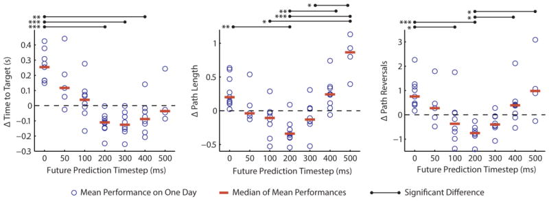
Online performance results from nine datasets where multiple future prediction time leads (τ) were tested on each day while we held the BMI controller’s level of delay constant at 200 ms. The differences between the mean performance in a given condition and the average level of performance on a given day are shown (blue circles), and the median of these means is also shown for each condition (red bars). Peak performance is reached around τ =200. The standard approach of predicting present intent is the leftmost condition (τ =0). The black bars indicate significant differences between conditions (p<0.05). Asterisks to the left of the bars indicate the level of significance (p<0.05, p<0.01, and p<0.001 for one, two, and three asterisks respectively).

3.3 Online Experiment 2: Performance Benefits of Future Prediction with Small Delays

The first online experiment shows that future prediction improved the performance of a BMI with a 200 ms delay. In this second online experiment, we aimed to determine if future prediction would also improve the performance of a BMI with a delay as small as 100 ms. The results show that for all 3 days, the monkey made faster, straighter, and smoother movements when the delay was mitigated by using future prediction, for both the 100 ms and 200 ms delay conditions (figure 6, significant decrease shown in Time to Target, Path length, and Path Reversal metrics). Pairwise Wilcoxon rank sum tests confirm that the difference between the median performance values is significant for each metric, day, and level of delay (p<0.05 in all cases, with individual p-values depicted in figure 6).

Figure 6.

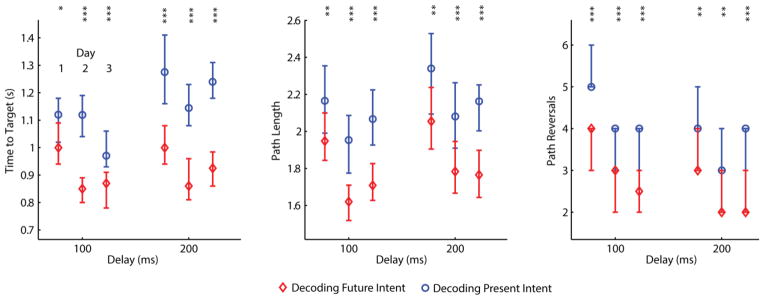
Online performance results for three different days and four different conditions tested on each day: (1) 100 ms delay, future prediction time lead τ =0, (2) 100 ms delay, τ =100, (3) 200 ms delay, τ =0, (4) 200 ms delay, τ =200. For each level of delay (horizontal axis), median performance for τ = 0 (blue circle) and for τ = 100 or 200 (red diamond) are shown, with 95% confidence intervals for the median. In the Path Reversals panel, the extremities of the confidence interval overlap with the median because the median value comprises a large proportion of the total number of observations (observations are integer values). Columns of asterisks indicate the level of significance for a comparison between the present prediction and future prediction condition (p<0.05, p<0.01, and p<0.001 for one, two, and three asterisks respectively).

On day 1, predicting into the future in the presence of 100 ms of delay decreased the median time needed to make a reach by 130 ms, decreased the median path length by 22% of the distance between the targets, and decreased the median amount of unnecessary path reversals by one. Results were similar for the other two experimental sessions as well. Predicting into the future in the presence of 200 ms of delay yielded greater performance benefits, but they were not twice as large as those seen for the 100 ms conditions.

3.4 Online Experiment 3: Effects of Pure Delay on BMI Performance and Future Prediction

In this experiment, we characterized the effect of “pure” delay (a delay added to the system with a buffer and therefore free of low-pass filter effects) on performance, and tested whether or not predicting into the future could compensate for a pure delay added in addition to the fixed delay of 100 ms from the PD controller. The results depicted in figure 7 show that there is a significant, deleterious effect of pure delay on performance for all metrics (significant, positive slope of the regression line predicting performance from delay, p<0.001), indicating that delay significantly decreases performance as expected. The effects of the pure delay are substantial. The slopes of the linear regressions predicting Δ Time to Target, Δ Path Length, and Δ Path Reversals from the number of milliseconds of delay indicate that every 100 ms of pure delay adds 185.5 ± 35.3 ms of additional time to the reach, 23.5 ± 10.3% additional path length, and 1.48 ± 0.24 additional path reversals (with ± indicating a 95% confidence interval). To understand the magnitude of these performance effects, it is useful to note that the average reach across all days for the condition with 0 ms of delay had a Time to Target of 1.38 s, a Path Length of 3.14, and a Path Reversal count of 5.78.

Figure 7.

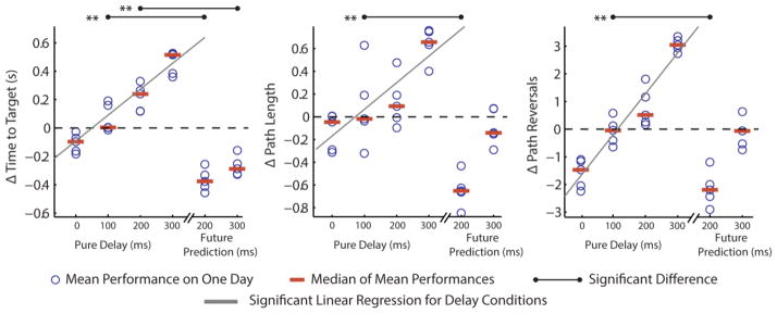
Online performance results from 5 datasets, with 6 conditions tested on each day, ordered as follows on the horizontal axis: (1) 0ms pure delay, (2) 100 ms pure delay, (3) 200 ms pure delay, (4) 300 ms pure delay, (5) 100 ms pure delay + a future prediction time lead (τ) of 200, (6) 200 ms pure delay + a future prediction time lead (τ) of 300. The differences between the mean performance for a given condition and the average level of performance on a given day are shown with blue circles, and the median of these means is plotted for each condition (red bars). Significant linear regressions predicting mean performance from pure delay (first four conditions) are shown in gray, while significant differences in the median of the mean performances between conditions 2 and 5, and conditions 3 and 6, are shown in black (p<0.01). Two effects are illustrated: the effect of pure delay (delay added to the system with a buffer) on performance (first four conditions), and the effect of predicting into the future to compensate for pure delay (condition 2 vs. condition 5, condition 3 vs. condition 6).

Pairwise comparisons between two of the pure delay conditions (pure delay = 100 ms; pure delay = 200 ms) and the two corresponding future prediction conditions (pure delay = 100 ms, τ =200; pure delay = 200 ms, τ =300) also show that predicting into the future significantly improves performance. For the condition where τ =200, the Δ Time to Target, Δ Path Length, and Δ Path Reversal metrics all show significant improvement (Wilcoxon rank sum test on the distributions of mean performances, p<0.01) These results indicate that future prediction can successfully compensate for “pure” delays unaccompanied by low-pass filter effects, in much the same way that performance improved in the other two online experiments. For the case of τ = 300, the Δ Time to Target metric shows a significant improvement (p<0.01) while the Δ Path Length and Δ Path Reversals metrics show no significant improvement, indicating that there is a limit to the amount of delay for which one can successfully compensate using future prediction.

4. Discussion

4.1 Effects of Future Prediction and Delay on Performance

Our offline results from two monkeys demonstrate that future movements can be accurately reconstructed from neural activity without much loss in fidelity up to a time lead of 200 ms, verifying the feasibility of predicting future intended movements (figure 4(a)). The offline results also suggest that future prediction can reduce the effective control delay in BMI systems, decreasing the delay by an amount equal to the future prediction time lead until the improvement begins to level off at 300 ms (figure 4(b)).

Our online results from one monkey confirm that decoding intended future movements and using them as a command signal for a BMI can significantly improve performance, making reaches faster, straighter, and smoother for a range of future prediction time leads (up to 300 ms) and delays (100, 200, and 300 ms). In the first online experiment, performed with a BMI that had a 200 ms control delay (in addition to the base level of delay added by our real-time BMI system), performance improved steadily as the future prediction time lead (τ ) was increased, peaking at τ = 200 ms (figure 5). Future prediction with τ = 200 ms decreased the time it took to complete the reach by 372 ms, decreased the path length by 56% of the distance between the targets, and eliminated 1.45 path reversals as compared to the typical present prediction strategy. In the second online experiment, we confirmed that future prediction yielded a substantial benefit in a BMI system with as little as 100 ms of delay (figure 6). Finally, in the third online experiment we showed that future prediction also significantly improved performance when compensating for delays caused by a buffer as opposed to delays with a low-pass filter effect (figure 7). Taken together, these 16 days of results show that it is possible to compensate for the negative effects of delay in BMI control loops through a simple solution that many algorithms in use today could incorporate with minimal difficulty.

In addition to exploring the benefits of future prediction, in our third online experiment, we also characterized the performance degradation of a BMI as a function of the amount of delay in the system. We showed that reaches took longer, became less smooth, and reversed directions more frequently as the amount of delay in the system increased (figure 7). The magnitude of this effect was large; linear regressions predicting performance from the amount of delay present revealed that every 100 ms of delay added 185.5 ± 35.3 ms of additional time to the reach, 23.5 ± 10.3% additional path length, and 1.48 ± 0.24 additional path reversals (with ± indicating a 95% confidence interval). This evidence confirms the idea that delay is deleterious to performance in BMIs, and that mitigation of delay is a likely mechanism for the improvement of performance. These results, while not unexpected, also highlight the importance of minimizing delay in BMIs, a subject which has not yet been a focus of serious study in the literature at the time of submission.

4.2 Mechanisms by which Future Prediction Improves Performance

We propose two different ways in which future prediction might lead to benefits in BMI performance and therefore might have caused the benefits that we found in this study. Both of the proposed benefits assume that future prediction decreases the effective delay in the BMI control loop. First, if the user’s desired arm state at τ ms into the future is decoded accurately, then, at the very least, the user should reach the target τ ms faster than if the user’s present intent had been decoded. This is because the user’s intent to reach towards a new target will be decoded and implemented by the BMI τ ms earlier. Second, if the user’s intent is decoded inaccurately and a correction must be made during the reach, the user will be able to both perceive the mistake and to make a correction more quickly than if present prediction had been used. This ability to make corrections more quickly will save the user an amount of time proportional to how many corrections are made during the reach. This could decrease the time needed to complete a reach by more than τ ms, as was observed in the first online experiment (reaches were completed 372 ms faster with 200 ms of future prediction), and could make the reaches smoother and more direct.

Both of these mechanisms assume that future prediction compensates for delay in BMIs. We have given strong evidence in favor of this assumption by demonstrating offline that our future prediction decoders can reduce the effective delay of a BMI, and by demonstrating online that delay reduces performance in BMIs and that future prediction can recover this lost performance. We are therefore confident that the first mechanism proposed above was responsible for some of the benefit seen. However, without an experiment specifically designed to do so, we cannot determine to what extent the second mechanism may have also been responsible for the performance improvement seen. Nevertheless, studies analyzing the effects of delayed feedback on reaching in healthy subjects consistently indicate that delay causes reaches to take longer and to be less accurate beyond what would be expected from simply increasing the reaction time of the reach by the amount of delay added (Shimada et al 2004, MacKenzie and Ware 1993). Therefore, if future prediction decreases delay, then we would expect a corresponding increase in performance.

4.3 A Comparison of Delays Encountered in BMIs and Healthy Reaching

We think it instructive to note that the control loop delay a user experiences when making reaches with a BMI is usually different than what a user experiences when making reaches with their own body. In the intact nervous system, sensory information returning from the periphery (i.e. the feedback component) can shape activity in M1 as soon as ~100 ms following somatosensory stimulation or ~200 ms following visual stimulation (Keele and Posner 1968, Flanders et al 1986, Spidalieri et al 1983). Since BMIs do not typically provide somatosensory information, and since the somatosensory feedback delay is smaller than the visual feedback delay, the feedback delay experienced during BMI use is usually higher than that experienced during healthy reaching.

In addition, the feedforward delays experienced during BMI use are typically larger than those experienced during healthy reaching. The average time between activity in M1 and subsequent movement of the upper limb during healthy reaching is typically 100ms (Paninski et al 2004, Schwartz et al 2004) and does not vary based on the modality of sensory feedback used to cue the start of movement (Lamarre et al 1983). The feedforward delay in BMI systems utilizing a physical end effector like a robotic or prosthetic arm is typically higher than the delay in the biological system (there is at least 180 ms of feedforward delay in our configuration), highlighting the need to improve the responsiveness of robotic/prosthetic systems and/or to use future prediction decoding. We do note, however, that some of the delay in our control loop (~50 ms) is due to the visual display that gives feedback to the monkey and would not be present if a real robotic arm were controlled instead of a simulated one.

4.4 Optimal Future Prediction Time Lead

We posit that decoding the user’s intent at a time lead greater than the amount of delay in the BMI control loop could lead to a response time even faster than that observed during healthy functioning. Suppose that performance increases as the future prediction time lead (τ) gets larger (as we have shown), but continues to increase even when τ is larger than the amount of delay in the BMI control loop. Then, the optimal τ should be the maximal τ at which any further increase causes a drop in decoding accuracy so large that performance degrades overall. In the first online experiment, we tested values of τ greater than the delay added to the BMI (200 ms), but found that performance peaked at τ=200, remained approximately equal at τ=300 and began to decrease at τ=400 and τ=500 (figure 5). However, we think that this is because the accuracy of the decoders begins to decrease steeply at τ=200 (figure 4(a)). Future work could test the hypothesis that the optimal future prediction time lead might be greater than the delay of the BMI system by testing BMIs with smaller delays.

4.5 Limitations of Straightness and Smoothness Metrics

Results from all three of the online experiments consistently showed that reaches were made straighter (decrease in Path Length metric) and smoother (decrease in Path Reversals metric) when future prediction was used. However, we emphasize here that a reach was defined to begin at the time immediately after the previous target was acquired; no attempt was made to compute a reaction time interval and to define the reach to begin after this interval had passed. Since our future prediction decoders may have decreased this reaction time interval by compensating for delays, reaches made with future prediction could appear straighter and smoother only because the distance traveled and the direction changes made during this reaction time period were decreased. It is therefore unclear whether or not the straightness and smoothness benefits resulted from a decreased reaction time, an improved reach quality after the initial reaction time interval, or both.

4.6 Limitations of Using Future Prediction to Offset Delay in BMIs

It is worth noting here that any delay in the BMI control system will put an absolute floor on how quickly the BMI will be able to react to a newly formed motor command, even if accurate future prediction is implemented. For example, consider a BMI that controls a computer cursor and that has a “pure” delay of 200 ms (as opposed to a delay from low-pass filtering). In this case, the cursor would be completely unable to move in response to a new movement command for at least 200 ms. However, when the command signal is executed 200 ms later, if it represents a future intent, then the cursor will “catch up” to the subject’s intention. This will never happen if the decoder predicts present intent.

4.7 Generalization beyond Our Decoding Algorithm

While our results were robust in that future prediction improved performance significantly on all 16 days tested, whether or not the results will generalize to different decoding algorithms and different tasks is unknown. One issue is that our decoding algorithm decodes hand position, while many other algorithms decode hand velocity (Taylor et al 2002, Velliste et al 2008, Kim et al 2008, Chadwick et al 2011). Since hand velocity changes more rapidly than hand position and is less well correlated with itself at nearby time points, we might expect future prediction decoders not to be able to decode hand velocity at as large of a time lead as they can decode hand position. We might also expect there to be less of a delay in changing the velocity of a robotic arm than there is in changing the position of a robotic arm. Other variables, such as joint torques or muscle activations, change more rapidly still. Nevertheless, neural activity in the motor cortex should still lead these variables, and we would expect that future prediction could still compensate for delays when decoding these variables even if the delay being mitigated is smaller.

Summary

This study is the first to characterize the effects of control delays in a BMI and to show that decoding the user’s future intent can compensate for the negative effect that control delay has on performance. Our offline results from two subjects show that future movements can be successfully decoded from neural activity at a time lead of up to 200 ms with minimal decrease in decoding accuracy, and that predicting future movements reduces the effective delay in a BMI system. Our online results from one subject show that, on all 16 days of experimentation, decoding future intended movement enabled the subject to make quicker, straighter, and smoother movements when controlling a simulated arm. Our online results also show that control delay significantly decreases BMI performance; every 100 ms of additional delay added 185.5 ± 35.3 ms of additional time to the average reach, 23.5 ± 10.3% additional path length, and 1.48 ± 0.24 additional path reversals (± 95% confidence interval).

References

- Björck Å. Numerical Methods for Least Square Problems. SIAM; 1996. [Google Scholar]
- Carmena JM, Lebedev MA, Crist RE, O’Doherty JE, Santucci DM, Dimitrov DF, Patil PG, Henriquez C, SNicolelis MAL. Learning to Control a Brain Machine Interface for Reaching and Grasping by Primates. PLoS Biology. 2003;1:e2. doi: 10.1371/journal.pbio.0000042. [DOI] [PMC free article] [PubMed] [Google Scholar]
- Cunningham JP, Nuyujukian P, Gilja V, Chestek CA, Ryu SI, Shenoy KV. A closed-loop human simulator for investigating the role of feedback control in brain-machine interfaces. J Neurophysiol. 2011;105:1932–49. doi: 10.1152/jn.00503.2010. [DOI] [PMC free article] [PubMed] [Google Scholar]
- Chadwick E, Blana D, Simeral J, Lambrecht J, Kim S, Cornwell A, Taylor D, Hochberg L, Donoghue J, Kirsch R. Continuous neuronal ensemble control of simulated arm reaching by a human with tetraplegia. Journal of Neural Engineering. 2011;8:034003. doi: 10.1088/1741-2560/8/3/034003. [DOI] [PMC free article] [PubMed] [Google Scholar]
- Fagg AH, Ojakangas GW, Miller LE, Hatsopoulos NG. Kinetic Trajectory Decoding Using Motor Cortical Ensembles. IEEE Transactions on Neural Systems and Rehabilitation Engineering. 2009;17:487–96. doi: 10.1109/TNSRE.2009.2029313. [DOI] [PubMed] [Google Scholar]
- Flanders M, Cordo PJ, Anson JG. Interaction between visually and kinesthetically triggered voluntary responses. J Mot Behav. 1986;18:427–48. doi: 10.1080/00222895.1986.10735389. [DOI] [PubMed] [Google Scholar]
- Foulkes AJM, Miall RC. Adaptation to visual feedback delays in a human manual tracking task. Experimental Brain Research. 2000;131:101–10. doi: 10.1007/s002219900286. [DOI] [PubMed] [Google Scholar]
- Gage GJ, Ludwig KA, Otto KJ, Ionides EL, Kipke DR. Naive coadaptive cortical control. Journal of neural engineering. 2005;2:52. doi: 10.1088/1741-2560/2/2/006. [DOI] [PubMed] [Google Scholar]
- Keele SW, Posner MI. Processing of visual feedback in rapid movements. Journal of Experimental Psychology. 1968;77:155–8. doi: 10.1037/h0025754. [DOI] [PubMed] [Google Scholar]
- Kennedy PR, Bakay RAE, Moore MM, Adams K, Goldwaithe J. Direct control of a computer from the human central nervous system. Rehabilitation Engineering, IEEE Transactions on. 2000;8:198–202. doi: 10.1109/86.847815. [DOI] [PubMed] [Google Scholar]
- Kim SP, Simeral JD, Hochberg LR, Donoghue JP, Black MJ. Neural control of computer cursor velocity by decoding motor cortical spiking activity in humans with tetraplegia. Journal of neural engineering. 2008;5:455. doi: 10.1088/1741-2560/5/4/010. [DOI] [PMC free article] [PubMed] [Google Scholar]
- Kim S-P, Simeral JD, Hochberg LR, Donoghue JP, Friehs GM, Black MJ. Point-and-Click Cursor Control With an Intracortical Neural Interface System by Humans With Tetraplegia. IEEE Transactions on Neural Systems and Rehabilitation Engineering. 2011;19:193–203. doi: 10.1109/TNSRE.2011.2107750. [DOI] [PMC free article] [PubMed] [Google Scholar]
- Lamarre Y, Busby L, Spidalieri G. Fast ballistic arm movements triggered by visual, auditory, and somesthetic stimuli in the monkey. I. Activity of precentral cortical neurons. J Neurophysiol. 1983;50:1343–58. doi: 10.1152/jn.1983.50.6.1343. [DOI] [PubMed] [Google Scholar]
- MacKenzie IS, Ware C. Proceedings of the INTERACT’93 and CHI’93 conference on Human factors in computing systems. 1993. Lag as a determinant of human performance in interactive systems; pp. 488–93. [Google Scholar]
- Miall RC, Jackson JK. Adaptation to visual feedback delays in manual tracking: evidence against the Smith Predictor model of human visually guided action. Experimental Brain Research. 2006;172:77–84. doi: 10.1007/s00221-005-0306-5. [DOI] [PubMed] [Google Scholar]
- Miall R, Weir D, Stein J. Visuomotor tracking with delayed visual feedback. Neuroscience. 1985;16:511–20. doi: 10.1016/0306-4522(85)90189-7. [DOI] [PubMed] [Google Scholar]
- Orsborn AL, Dangi S, Moorman HG, Carmena JM. Closed-Loop Decoder Adaptation on Intermediate Time-Scales Facilitates Rapid BMI Performance Improvements Independent of Decoder Initialization Conditions. IEEE Transactions on Neural Systems and Rehabilitation Engineering. 2012;20:468–77. doi: 10.1109/TNSRE.2012.2185066. [DOI] [PubMed] [Google Scholar]
- Paninski L, Fellows MR, Hatsopoulos NG, Donoghue JP. Spatiotemporal Tuning of Motor Cortical Neurons for Hand Position and Velocity. Journal of Neurophysiology. 2003;91:515–32. doi: 10.1152/jn.00587.2002. [DOI] [PubMed] [Google Scholar]
- Schwartz AB, Moran DW, Reina GA. Differential Representation of Perception and Action in the Frontal Cortex. Science. 2004;303:380–3. doi: 10.1126/science.1087788. [DOI] [PubMed] [Google Scholar]
- Serruya MD, Hatsopoulos NG, Paninski L, Fellows MR, Donoghue JP. Brain-machine interface: Instant neural control of a movement signal. Nature. 2002;416:141–2. doi: 10.1038/416141a. [DOI] [PubMed] [Google Scholar]
- Shimada S, Hiraki K, da Matsuda GOI. Decrease in prefrontal hemoglobin oxygenation during reaching tasks with delayed visual feedback: a near-infrared spectroscopy study. Cognitive brain research. 2004;20:480–90. doi: 10.1016/j.cogbrainres.2004.04.004. [DOI] [PubMed] [Google Scholar]
- Spidalieri G, Busby L, Lamarre Y. Fast ballistic arm movements triggered by visual, auditory, and somesthetic stimuli in the monkey. II. Effects of unilateral dentate lesion on discharge of precentral cortical neurons and reaction time. J Neurophysiol. 1983;50:1359–79. doi: 10.1152/jn.1983.50.6.1359. [DOI] [PubMed] [Google Scholar]
- Suminski AJ, Tkach DC, Fagg AH, Hatsopoulos NG. Incorporating feedback from multiple sensory modalities enhances brain machine interface control. The Journal of Neuroscience. 2010;30:16777–87. doi: 10.1523/JNEUROSCI.3967-10.2010. [DOI] [PMC free article] [PubMed] [Google Scholar]
- Taylor DM, Tillery SIH, Schwartz AB. Direct Cortical Control of 3D Neuroprosthetic Devices. Science. 2002;296:1829–32. doi: 10.1126/science.1070291. [DOI] [PubMed] [Google Scholar]
- Tkach D, Reimer J, Hatsopoulos NG. Congruent activity during action and action observation in motor cortex. The Journal of Neuroscience. 2007;27:13241–50. doi: 10.1523/JNEUROSCI.2895-07.2007. [DOI] [PMC free article] [PubMed] [Google Scholar]
- Velliste M, Perel S, Spalding MC, Whitford AS, Schwartz AB. Cortical control of a prosthetic arm for self-feeding. Nature. 2008;453:1098–101. doi: 10.1038/nature06996. [DOI] [PubMed] [Google Scholar]
- Willett FR, Suminski AJ, Fagg AH, Hatsopoulos NG. Compensating for delays in brain-machine interfaces by decoding intended future movement. 34th Annu. Int. Conf. of the IEEE EMBS; San Diego, CA, USA. 2012. pp. 4087–4090. [DOI] [PubMed] [Google Scholar]