A Kernel of Truth: Statistical Advances in Polygenic Variance Component Models for Complex Human Pedigrees

Abstract

Statistical genetic analysis of quantitative traits in large pedigrees is a formidable computational task due to the necessity of taking the non-independence among relatives into account. With the growing awareness that rare sequence variants may be important in human quantitative variation, heritability and association study designs involving large pedigrees will increase in frequency due to the greater chance of observing multiple copies of rare variants amongst related individuals. Therefore, it is important to have statistical genetic test procedures that utilize all available information for extracting evidence regarding genetic association. Optimal testing for marker/phenotype association involves the exact calculation of the likelihood ratio statistic which requires the repeated inversion of potentially large matrices. In a whole genome sequence association context, such computation may be prohibitive. Toward this end, we have developed a rapid and efficient eigensimplification of the likelihood that makes analysis of family data commensurate with the analysis of a comparable sample of unrelated individuals. Our theoretical results which are based on a spectral representation of the likelihood yield simple exact expressions for the expected likelihood ratio test statistic (ELRT) for pedigrees of arbitrary size and complexity. For heritability, the ELRT is:

$$-\sum \text{ln}[1+{ĥ}^2({\lambda }_{gi}-1)],$$

where ĥ² and λ_gi are respectively the heritability and eigenvalues of the pedigree-derived genetic relationship kernel (GRK). For association analysis of sequence variants, the ELRT is given by

$$ELRT[h_q^2>0:\text{unrelateds}]-\left(ELRT\right[h_t^2>0:\text{pedigrees}]-ELRT[h_r^2>0:\text{pedigrees}\left]\right),$$

where $h_t^2,h_q^2$, and $h_r^2$ are the total, quantitative trait nucleotide, and residual heritabilities, respectively. Using these results, fast and accurate analytical power analyses are possible, eliminating the need for computer simulation. Additional benefits of eigensimplification include a simple method for calculation of the exact distribution of the ELRT under the null hypothesis which turns out to differ from that expected under the usual asymptotic theory. Further, when combined with the use of empirical GRKs—estimated over a large number of genetic markers— our theory reveals potential problems associated with non positive semi-definite kernels. These procedures are being added to our general statistical genetic computer package, SOLAR.

I. INTRODUCTION

With the rise of next generation sequencing (NGS) and the resulting increase in available whole genome sequence (WGS), the modern statistical genetics of complex disease-related phenotypes finds itself confronted with the Herculean task of analyzing an astronomical volume of data. Of particular importance is the fact that, by far, most human sequence variation is rare (1000 Genome Project Consortium et al., 2012), so rare that much sequence variation is effectively private (or lineage-specific). That fraction of the genome that we are most interested in, the phenotypically functional component, is even more likely to be dominated by such rare variation. In man, rare functional variation is best studied in large pedigrees. Basically, pedigree-based studies represent an implicit enrichment strategy for identifying and studying rare functional variants. Mendelian transmissions from parents to offspring maximize the chance that multiple copies of rare variants exist in the pedigree. Alternatively, studies of unrelated individuals like those typically performed in the now receding genome-wide association (GWA) era that has focused only upon common sequence variation can never capture more than one copy of a “private” variant. Whilst there are accumulating methods to examine the joint effects of sequence variation in a gene-centric manner that may be of value in the study of unrelateds, a large part of human genetics will stay focused on the rapid identification of specific rare variants of moderate to large effect on disease risk since such variants more rapidly lead to functional experimental validation and causal gene discovery with all of its concomitant benefits. Thus, it is apparent that the coming WGS era of human genetics will require a return to our fundamental roots with a refocus on pedigree-based studies of phenotypic variation (Blangero, 2004; Ott et al., 2011).

The analysis of the most valuable kinds (for studying rare variation) of large and complex human pedigrees has its own difficulties including substantial statistical and computational issues. At first glance, it would seem anachronistic to attack this issue by retreating to the classical methods of polygenic analysis under a variance components (VC) model, which have their origins almost a century ago now in Fisher (1918). This linear mixed model which allows for the simultaneous analysis of both fixed (e.g., the effects of specific sequence variants on the mean) and random effects (typically the residual polygenic effects and random environmental effects) has been successfully used for many years in human pedigree analysis. However, usage of VC models in large human pedigrees of the kind most likely to be valuable for the study of rare sequence variation has generally been computationally formidable. Similarly, obtaining accurate pedigree information itself is a difficult task in human populations (and especially isolated populations).

In this work, we demonstrate two advances in polygenic VC analysis that can be used to rationally analyze whole genome sequence variation in relation to its effects on phenotypic variation or disease risk. Specifically, we describe an eigenvalue decomposition (EVD) approach to likelihood analysis under a VC polygenic model (hereafter polygenic model) that greatly simplifies/speeds analyses and, more importantly, leads to a remarkable set of closed form analytical equations for power analyses for both heritability studies and marker-based association studies in arbitrary pedigrees. Additionally, this spectral decomposition of the likelihood function effectively removes all barriers to computation for even the largest and most complex of pedigrees. We also describe the use of empirical genetic relationship kernels (GRKs) that substantially broadens the potential to use polygenic models in the absence (or in support) of accurate pedigree information. We tie the two approaches together in a section where we use the EVD-derived likelihood approach to study the statistical properties of a typical GRK usage.

II. VARIANCE COMPONENTS MODELS

A. Standard polygenic model

We start with a standard description of the linear model for a phenotype vector under a VC model, which is a standard modeling approach for human family data (Almasy and Blangero, 1998; Blangero et al., 2001; Lange, 2002; Almasy and Blangero, 2010):

$${\mathbf{y}}_{n\times 1}={\mathbf{X}}_{n\times j}{\mathbf{\beta }}_{j\times 1}+\mathbf{g}+\mathbf{e},$$ (1)

where y, the phenotype vector of interest, X, a design matrix of covariate effects, and β, a vector of regression coefficients, are of dimensions n × 1, n × j, and j × 1, respectively, and n and j give the numbers of individuals in the pedigree and of fixed effects parameters, respectively; and g, and e are unobserved vectors of random genetic and environmental effects, respectively. On assuming that the genetic and environmental effects are uncorrelated, the polygenic model for the phenotypic covariance matrix is as follows:

$$V\left[\mathbf{y}\right]=\mathbf{\Sigma }=\mathbf{K}{h}^2+\mathbf{I}(1-h^2),$$ (2)

where K is the GRK (which is also known as a genetic relationship matrix), I is the identity matrix, and $h^2=\frac{{\sigma }_g^2}{({\sigma }_g^2+{\sigma }_e^2)}=\frac{{\sigma }_g^2}{{\sigma }_p^2}$ is the standard additive genetic heritability, where ${\sigma }_g^2,{\sigma }_e^2$, and ${\sigma }_p^2$ are the additive genetic, residual environmental, and total phenotypic variances, respectively. For this basic model, K = 2Φ, where Φ is the expected kinship matrix generally derived directly from pedigree information. Assuming that the trait follows a multivariate normal (MVN) distribution, the model ln-likelihood function is given as:

$$\text{ln}L(\mathbf{\beta },h^2|\mathbf{y},\mathbf{X})=-\frac{1}{2}[N\text{ln}2\pi +\text{ln}|\mathbf{\Sigma }|+\mathbf{\delta }\prime {\mathbf{\Sigma }}^{-1}\mathbf{\delta }],$$ (3)

where δ = y − Xβ. If the data do not conform to the MVN assumption, we generally advocate direct inverse Gaussian transformation either prior to analysis or post initial covariate adjustment.

Following Boerwinkle et al. (1986), a measured genotype (MG) effect at a single nucleotide polymorphism (SNP) may be included in the model for the mean as a fixed-effect parameter. Earlier approaches to incorporate a MG effect were made by Moll et al. (1979) as a fixed effect and by Hopper and Matthews (1982) as a random effect, but the mature MG model was fully developed by Boerwinkle et al. (1986). Casual inspection of the likelihood equation (Eq. 3) shows that likelihood analysis to the tune of one SNP at a time can be computationally burdensome for a large number of SNPs, and for large pedigrees. This is because computation of the inverse covariance matrix of the pedgiree is required each time the likelihood is maximized in order to find the maximum likelihood estimates (MLEs). In current GWA study designs employing large extended families and having total sample sizes of about a thousand (or appreciably more) individuals, and where a million SNPs are to be analyzed, we would have to invert the covariance matrix of size say 1000×1000 for at least 1M×(number of likelihood evaluations) times. Obviously, this problem is amplified for NGS data analysis where the number of sequence variants to be analyzed can easily approach 25M in a study of similar size.

B. Eigensimplification of the MVN likelihood

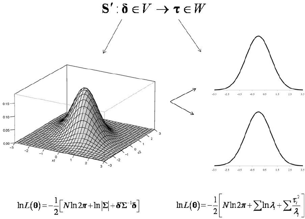
Because of the computational burden inherent in the traditional analytical approach, we earlier proposed a simplified approach to the problem using the EVD of the covariance matrix (Dyer et al., 2009). We call this general process the eigensimplification of the likelihood function. Hints or variations of the basic EVD method have been developed in relation to maximum likelihood estimation, and have been applied in statistics and genetics for decades, always as a means of simplifying the attendant computational rigor (Patterson and Thompson, 1971; Thompson, 1973, 2008; Dempster et al., 1984; Thompson and Cameron, 1986; Thompson and Meyer, 1986; Thompson and Shaw, 1990, 1992, Kang et al., 2008, 2010). Here we similarly employ an orthogonal transformation of the data vector which maps or linearly transforms a vector of non-independent observations to a vector of independent observations. If the trait data was sampled from unrelated individuals, the likelihood would involve the simple product of univariate normal densities. However, because data sampled from families are inherently non-independent, we must of account for the non-independence generated by genetic transmission. After the orthogonal transformation, we will see that the data are "decorrelated" or “whitened”, which essentially diagonalizes the covariance matrix and reduces the likelihood again to the product of univariate normal densities. This consequence arises simply because the data vector has been taken from a vector space of non-independent observations into a vector space of independent observations by way of an orthogonal transformation to the eigenbasis. Figure 1 represents a graphic depiction of this process where a bivariate probability density is transformed into two univariate probability densities.

Figure 1.

Orthogonal transformation the residuals vector. Schematic representation of the linear mapping of a vector in vector space V (of non-independent data) to a vector in vector space W (of independent data).

Assuming for convenience and with complete generality that ${\sigma }_p^2=1$, the EVD of the covariance matrix can be written as:

$$\mathbf{\Sigma }=\mathbf{S}{\mathbf{D}}_p\mathbf{S}\prime =\mathbf{S}[h^2{\mathbf{D}}_g+(1-h^2\left)\mathbf{I}\right]\mathbf{S}\prime =\mathbf{S}[\mathbf{I}+h^2({\mathbf{D}}_g-\mathbf{I}\left)\right]\mathbf{S}\prime ,$$ (4)

where S is an orthogonal matrix of eigenvectors, and D_p = diag {λ_pi} and D_g = diag {λ_gi} are respectively diagonal matrices of phenotypic and additive genetic eigenvalues. The simple linear form for the phenotypic eigenvalues represents the critical component leading to dramatic speed-up of likelihood function evaluation. Likelihood computations can now be greatly simplified by employing a linear transformation of the vector of residuals to the eigenbasis of the covariance matrix, which we denote by τ:

$$\mathbf{\tau }=\mathbf{S}\prime \mathbf{\delta }.$$ (5)

Since δ is multivariate normal, then so is the vector of transformed variables (Anderson, 1984):

$$\mathbf{\tau }=N(\mathbf{S}\prime \mathbf{\mu },\mathbf{S}\prime \mathbf{\Sigma }\mathbf{S}),$$

where V [τ] = S′ΣS = I. One of the chief virtues of this approach, besides leading to a simplified likelihood, is that S and D_g can be computed from an initial EVD of K which needs to be performed only once before subsequent model evaluations. That the EVD of K is sufficient for our purposes is made possible by the facts that the eigenvectors of Σ are also the eigenvectors of K (Thompson and Shaw, 1990, 1992), and the eigenvalues of Σ can be written as a linear function of the eigenvalues of K in the manner stated above. From standard multivariate theory (Stuart and Ord, 1987), we know that the full likelihood is factored into the likelihood for the transformed trait and the likelihood for the transformation, where the latter is given by the Jacobian of the transformation, which is denoted by J_δ→τ. Thus, the full likelihood will be on the natural logarithmic scale a sum of the likelihood of the transformed variable and the natural logarithm of the Jacobian of the transformation:

$$\text{ln}L(\mathbf{\theta }|\mathbf{y},\mathbf{X})=\text{ln}L(\mathbf{\tau })+\text{ln}(J_{\mathbf{\delta }\to \mathbf{\tau }})=-\frac{1}{2}[\text{ln}|\mathbf{S}\prime \mathbf{\Sigma }\mathbf{S}|+\mathbf{\tau }\prime {(\mathbf{S}\prime \mathbf{\Sigma }\mathbf{S})}^{-1}\mathbf{\tau }]+\text{ln}(J_{\mathbf{\delta }\to \mathbf{\tau }})=-\frac{1}{2}[\text{ln}|\mathbf{S}\prime (\mathbf{S}{\mathbf{D}}_p\mathbf{S}\prime \left)\mathbf{S}\right|+\mathbf{\tau }\prime {(\mathbf{S}\prime (\mathbf{S}{\mathbf{D}}_p\mathbf{S}\prime \left)\mathbf{S}\right)}^{-1}\mathbf{\tau }]+\text{ln}|\mathbf{S}\prime |=-\frac{1}{2}[\text{ln}|\mathbf{I}{\mathbf{D}}_p\mathbf{I}|+\mathbf{\tau }\prime {\left(\mathbf{I}{\mathbf{D}}_p\mathbf{I}\right)}^{-1}\mathbf{\tau }]=-\frac{1}{2}[\text{ln}|\mathbf{I}+h^2({\mathbf{D}}_g-\mathbf{I}\left)\right|+\mathbf{\tau }\prime {[\mathbf{I}+h^2({\mathbf{D}}_g-\mathbf{I}\left)\right]}^{-1}\mathbf{\tau }]=-\frac{1}{2}\sum \text{ln}[1+h^2({\lambda }_{gi}-1)]-\frac{1}{2}\sum \frac{{\tau }_1^2}{1+h^2({\lambda }_{gi}-1)},$$ (6)

where θ = [β, h²]′ is the parameter vector, S′S = SS′ = I by definition of an orthogonal matrix, |S′| = 1 on restricting S′ to be a rotation (Pettofrezzo, 1978; Abadir and Magnus, 2005), and the summations are taken over n. Note that the phenotypic eigenvalues are re-expressed as a function of the heritability and the additive genetic eigenvalues. The major result of this spectral decomposition is that the likelihood has been simplified to be a sum of univariate likelihoods, as would be the case for the total likelihood for a sample of unrelated individuals or independent observations. It is interesting to observe that similar simplified likelihoods have been proposed under similar conditions involving the eigenvalues of the covariance matrix (Anderson and Olkin, 1985), but to our knowledge it appears that these simplified likelihoods were not utilized until only recently in statistical genetics in the context of the linear mixed model (Kang et al., 2008). Importantly, we note that because of the linear simplicity of Eq. 4, the required spectral decomposition of the GRK needs to be done only once and the transformation can be performed on the phenotype and covariate vector prior to analysis. For real data, this will be even true across the evaluation of very different models as long as the missing data pattern (for both phenotype and covariates) is constant. This fact was not noted nor implemented by Kang et al (2008). Remarkably, our eigensimplification of the likelihood results in a rapid exact calculation of the usual MVN likelihood that is equivalent in speed to that observed for an equal number of unrelated subjects.

III. EXPECTED LIKELIHOOD RATIO TEST STATISTICS

A. Heritability

The eigensimplification of the multivariate likelihood in Eq.(6) leads to some very useful analytical results of substantial relevance for the genetic analysis of phenotypic variation in arbitrary pedigrees. To show some of these results, it is convenient to work with the expected likelihood ratio test statistic, denoted as ELRT. We employ the ELRT for several reasons: 1) it is the easiest test statistic to analytically derive in comparison to asymptotically equivalent alternatives, 2) it provides an asymptotically uniformly most powerful test statistic for a variance component and, 3) the ELRT leads to dramatically simplified analytical power and ARE analyses.

To derive the ELRT, we require the following expectation:

$$E(\mathbf{\tau }\prime {(\mathbf{S}\prime \mathbf{\Sigma }\mathbf{S})}^{-1}\mathbf{\tau })=E\left(Tr\right(\mathbf{\tau }\prime {(\mathbf{S}\prime \mathbf{\Sigma }\mathbf{S})}^{-1}\mathbf{\tau }\left)\right)=E\left(Tr\right({(\mathbf{S}\prime \mathbf{\Sigma }\mathbf{S})}^{-1}\mathbf{\tau }\mathbf{\tau }\prime \left)\right)=Tr\left(E\right({(\mathbf{S}\prime \mathbf{\Sigma }\mathbf{S})}^{-1}\mathbf{\tau }\mathbf{\tau }\prime \left)\right)=Tr\left({(\mathbf{S}\prime \mathbf{\Sigma }\mathbf{S})}^{-1}E\right(\mathbf{\tau }\mathbf{\tau }\prime \left)\right)=Tr\left({(\mathbf{S}\prime \mathbf{\Sigma }\mathbf{S})}^{-1}E\right(\mathbf{S}\prime \mathbf{\delta }(\mathbf{S}\prime \mathbf{\delta })\prime \left)\right)=Tr({(\mathbf{S}\prime \mathbf{\Sigma }\mathbf{S})}^{-1}\mathbf{S}\prime E(\mathbf{\delta }\mathbf{\delta }\prime \left)\mathbf{S}\right)=Tr({(\mathbf{S}\prime \mathbf{\Sigma }\mathbf{S})}^{-1}\mathbf{S}\prime \mathbf{\Sigma }\mathbf{S})=Tr\left(\mathbf{I}\right)=n,$$

which shows that the quadratic term in the likelihood function cancels out on taking the difference in the ELRT. Thus, for a test of total additive genetic heritability we find:

$$ELRT[{ĥ}^2>0]=E[-2(\text{ln}L(h_0^2=0)-\text{ln}L\left({ĥ}^2\right)\left)\right]=E[-2(-\frac{1}{2}[\text{ln}|\mathbf{S}\prime {\mathbf{\Sigma }}_N\mathbf{S}|+\mathbf{\tau }\prime {(\mathbf{S}\prime {\mathbf{\Sigma }}_N\mathbf{S})}^{-1}\mathbf{\tau }]+\frac{1}{2}[\text{ln}|\mathbf{S}\prime {\mathbf{\Sigma }}_A\mathbf{S}|+\mathbf{\tau }\prime {(\mathbf{S}\prime {\mathbf{\Sigma }}_A\mathbf{S})}^{-1}\mathbf{\tau }]\left)\right]=\left(\text{ln}\right|{\mathbf{D}}_{pN}|+\mathbf{I})-\left(\text{ln}\right|{\mathbf{D}}_{pA}|+\mathbf{I})=\text{ln}|\mathbf{I}+h_0^2({\mathbf{D}}_g-\mathbf{I}\left)\right|-\text{ln}|\mathbf{I}+{ĥ}^2({\mathbf{D}}_g-\mathbf{I})|=-\sum \text{ln}[1+{ĥ}^2({\lambda }_{gi}-1)],$$ (7)

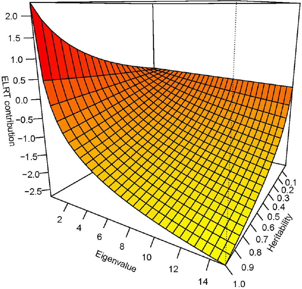
where the covariance matrices, and diagonal matrices of phenotypic eigenvalues under the null and alternative hypotheses are respectively subscripted by N and A, and $h_0^2$ and ĥ² denote the heritabilities under the null and alternative hypotheses, respectively. The relationship between the heritabilities and the eigenvalues in relation to the function in the summand is depicted in Figure 2. Because of the negative sign outside the summation, eigenvalues less than 1 contribute positively to the ELRT while those greater than 1 decrease the ELRT. This makes intuitive sense since eigenvalues below 1 are direct indications of correlation amongst individuals. This remarkably simple formula provides the expected test statistic for heritability in pedigrees of arbitrary size and complexity as a function of the easily obtained eigenvalues of the GRK which will often be the pedigree-derived coefficient of relationship matrix. This is the first general formula for pedigree-based heritability testing that we know of. It proves to be a very simple foundation for calculating power to detect heritability.

Figure 2.

Contribution to the ELRT as a function of the eigenvalues and heritabilities.

B. Association in the Presence of Residual Heritability

Given that association testing of specific sequence variants is often the focus of genetic analysis of human disease-related phenotypic variation, the simplification provided by Eq.(6) can also be used to derive the ELRT required for fixed effect testing of marker association. The effect of a sequence variant through a fixed MG effect influencing the mean, can be revisualized as a component of genetic variance. Basically, inference on a fixed effect parameter can be made by examining the perturbation to the variance due to presence of the fixed effect. This approach is used universally in standard linear regression analysis. Recall that an F statistic is essentially a ratio of variances. For a standard F-test on a regression coefficient, the variance explained by the regression is compared to the unexplained variance. If the regression parameter is significant (i.e. if the fixed effect is statistically important), it will perturb the variance, or rather, increase the ratio of the explained to the unexplained variance. Similarly, for the ELRT, we can make an inference on the significance of a SNP effect by way of the perturbation to the variance due to the SNP.

The foregoing requires a measure of the variance component due to the sequence variant. The modeling of a variance component due to a single variant has been addressed by many investigators in human genetics (Hopper and Mathews, 1982; Boerwinkle and Sing, 1986, 1987; Blangero et al., 2000; Blangero et al., 2005). Here we will use a simple (but widely biologically valid) model employing additive gene action. Consider now a single diallelic locus representative of a quantitative trait nucleotide (QTN) where the alleles have frequencies p and (1 − p). From classical theory, the QTN variance, denoted by ${\sigma }_q^2$, is known to be:

$${\mathrm{\sigma }}_q^2=2p(1-p)a^2,$$ (8)

where a is the displacement between genotypic means. The QTN-specific heritability, denoted by $h_q^2$, is therefore given as:

$$h_q^2=\frac{{\mathrm{\sigma }}_q^2}{{\mathrm{\sigma }}_p^2}.$$ (9)

We use this to define the residual heritability, denoted by $h_r^2$, which is given as:

$$h_r^2=\frac{h_t^2-h_q^2}{1-h_q^2},$$ (10)

where $h_t^2$ is the total heritability. The residual heritability measures the relative amount of additive genetic variation left after accounting for the QTN effect (and any other covariate effects in the model).

Let the covariance matrices under the null and alternative be respectively given as:

$${\mathbf{\Sigma }}_N=[2\mathbf{\Phi }{h}_t^2+(1-h_t^2\left)\mathbf{I}\right]{\sigma }_p^2,$$ (11)

and

$${\mathbf{\Sigma }}_A=[2\mathbf{\Phi }{h}_r^2+(1-h_r^2\left)\mathbf{I}\right]{\sigma }_p^2(1-h_q^2).$$ (12)

Thus, using the eigensimplification of the MVN likelihood, we find for testing association with a sequence variant:

$$ELRT[h_q^2>0:\text{pedigrees}]=E[-2(\text{ln}L(h_q^2=0)-\text{ln}L(h_q^2>0)\left)\right]=n\text{ln}{\sigma }_p^2+\sum \text{ln}[1+h_t^2({\lambda }_{gi}-1\left)\right]-n\text{ln}{\sigma }_p^2-n\text{ln}(1-h_q^2)-\sum \text{ln}[1+h_r^2({\lambda }_{gi}-1\left)\right]=-n\text{ln}(1-h_q^2)+\sum \text{ln}[1+h_t^2({\lambda }_{gi}-1\left)\right]-\sum \text{ln}[1+h_r^2({\lambda }_{gi}-1\left)\right]=ELRT[h_q^2>0:\text{unrelates}]-\left(ELRT\right[h_t^2>0:\text{pedigrees}]-ELRT[h_r^2>0:\text{pedigrees}\left]\right),$$ (13)

where we express the last form of the statistic in terms of the expected statistics for the QTN-specific heritability in a sample of unrelateds, the total heritability in pedigrees, and the residual heritability in pedigrees, respectively. Eq.(13) provides for the first time a completely general analytical formula for calculating expected association test statistics (and hence power) in arbitrary pedigrees. This formula obviates the need for extensive computer simulation which has been the usual method for obtaining power for association studies on pedigrees. Consistent with conventional wisdom regarding association testing (Visscher et al., 2008), the last formulation shows the power to detect association in pedigrees will be less than or at most equal to that in a sample of unrelateds. Eq.(13) should prove of substantial value in study design of pedigree-based association studies.

IV. POWER AND ASYMPTOTIC RELATIVE EFFICIENCY

A. Power

Power can be computed as the probability integral from the point on the alternative distribution corresponding to the nominal significance level or alpha (on the null distribution) to the upper limit of the alternative distribution at positive infinity. Since the total probability of any distribution is 1, power can be conveniently computed as:

$$\text{Pr}({ĥ}^2>0)=\underset{{\chi }_{\alpha ;\nu ,\xi =0}^2}{\overset{\infty }{\int }}d{\chi }_{\nu ,\xi }^2=\underset{0}{\overset{\infty }{\int }}d{\chi }_{\nu ,\xi }^2-\underset{0}{\overset{{\chi }_{\alpha ;\nu ,\xi =0}^2}{\int }}d{\chi }_{\nu ,\xi }^2=1-\underset{0}{\overset{{\chi }_{\alpha ;\nu ,\xi =0}^2}{\int }}d{\chi }_{\nu ,\xi }^2=1-\beta ,$$ (14)

where the distribution under the alternative hypothesis is the non-central chi-square distribution, denoted by ${\chi }_{\nu ,\xi }^2$, ν is the degrees of freedom (d.f.) parameter, ξ is the non-centrality parameter (NCP), ${\chi }_{\alpha ;\nu ,\xi =0}^2$ is the point on the non-central chi-square distribution corresponding to the 100(1 − α) percentage point on the distribution under the null hypothesis, and $\beta =\underset{0}{\overset{{\chi }_{\alpha ;\nu ,\xi =0}^2}{\int }}d{\chi }_{\nu ,\xi }^2$ is the probability of making a type II error (with apologies for the double use of beta).

When ξ = 0 the non-central chi-square degenerates to the usual chi-square, which is the distribution of the test statistic under the null hypothesis. For standard test cases (e.g. regression coefficients), alpha is the nominal significance level, and so the threshold value for the variate corresponding to the significance level is given as:

$$\alpha =0.05\le \text{Pr}(\beta =0)=\text{Pr}\left({\chi }_1^2\right),$$

which gives a threshold chi-square of ${\chi }_1^2={\chi }_{\alpha ;\nu ,\xi =0}^2\cong 3.84146$. This is modified, however, under non-standard test cases, as in a null hypothesis on the heritability, where the null lies on a boundary of the parameter space. For such cases (and assuming that the variates are independently and identically distributed (i.i.d.)), it is known that the statistic is asymptotically distributed as follows (Chernoff, 1954; Miller, 1977; Self and Liang, 1987; Stram and Lee, 1994; Verbeke and Molenberg, 2003; Dominicus et al., 2006; Visscher, 2006; DasGupta, 2008; Giampaoli and Singer, 2009):

$$LRT=\frac{1}{2}{\chi }_0^2+\frac{1}{2}{\chi }_1^2,$$

which is a 50:50 mixture of a variate with a point-mass at 0, denoted by ${\chi }_0^2$, and a chi-square with 1 d.f., denoted by ${\chi }_1^2$. Consequently, this upwardly modifies the effective test size:

$$\alpha =0.05\le \text{Pr}(h^2=0)\frac{1}{2}\text{Pr}\left({\chi }_0^2\right)+\frac{1}{2}\text{Pr}\left({\chi }_1^2\right)\Rightarrow 2\alpha =1.0\le 0+\text{Pr}\left({\chi }_1^2\right),$$

which gives a threshold chi-square of ${\chi }_1^2={\chi }_{2\alpha ;\nu ,\xi =0}^2\cong 2.70554$ (Visscher, 2006). We will revisit this asymptotic distribution of the LRT in a later section of the paper and show that it is generally conservative.

There are two general methods to calculate power in likelihood analysis owing to the fact that there are two approximations of the NCP for the non-central chi-square statistic (Brown et al., 1999). The older of the two approximations was first derived by Wald (1943) and is equal to the Wald statistic. Although the Wald statistic approximation to the NCP has been commonly used in statistical genetics (Williams and Blangero, 1999a&b; Blangero et al., 2001), the requirement of the expected Fisher information matrix makes it burdensome to compute. For the second, work by several investigators has shown that a reasonable NCP approximation is provided by the ELRT (Self et al., 1992; Liu, 1998; Brown et al., 1999; Sham et al., 2000, 2002; Rijsdijk et al., 2001). It will be more convenient to use the ELRT in the ensuing power analysis.

B. Asymptotic relative efficiency

The concept of asymptotic relative efficiency (ARE) is closely related to power. For two test statistics, denoted by T₁ and T₂, the ARE is defined as the ratio, n₁/n₂, where n₁ and n₂ are the respective theoretical sample sizes for T₁ and T₂ to attain the same power at the same alpha against the same alternative (DasGupta, 2008). Currently, there is no known analytic formula to compute these theoretical sample sizes, but several estimates of the ratio have been developed, one of which will be used here, namely the Pitman ARE (Pitman, 1948; cited in Noether, 1950, 1955), denoted as e_p. We give the definition of the Pitman ARE for comparing for T₁ to T₂ as (DasGupta, 2008):

$$e_p={(\underset{n\to \delta }{\text{lim}}\frac{\sqrt{n}{\sigma }_{{\theta }_1}}{{\mu }_{{\theta }_1}}/\underset{n\to \delta }{\text{lim}}\frac{\sqrt{n}{\sigma }_{{\theta }_2}}{{\mu }_{{\theta }_2}})}^2=\frac{{\sigma }_{{\theta }_1}^2}{{\sigma }_{{\theta }_2}^2}{\left(\frac{{\mu }_{{\theta }_2}}{{\mu }_{{\theta }_1}}\right)}^2=\frac{{\sigma }_{{\theta }_1}^2}{{\sigma }_{{\theta }_2}^2}{\left(\frac{{\mathrm{\theta ̂}}_2}{{\mathrm{\theta ̂}}_1}\right)}^2,$$ (15)

where the components are subscripted by test number, and the asymptotic parameter means are equivalent to the parameter MLEs. For many cases, the parameter standard errors (and hence their variances) are test-specific whereas the parameter means or MLEs are asymptotically equivalent (DasGupta, 2008). Thus, for such cases, including the current situation, e_p is given as the ratio of the variances.

The latter most form leads directly to the following useful result:

$$e_p=\frac{{\sigma }_{{\theta }_1}^2}{{\sigma }_{{\theta }_2}^2}{\left(\frac{{\mathrm{\theta ̂}}_2}{{\mathrm{\theta ̂}}_1}\right)}^2=\frac{{\mathrm{\theta ̂}}_2^2}{{\sigma }_{{\theta }_2}^2}/\frac{{\mathrm{\theta ̂}}_1^2}{{\sigma }_{{\theta }_1}^2}=\frac{W_2}{W_1}=\frac{NC{P}_2}{NC{P}_1},$$ (16)

where W․is the Wald statistic. We emphasize that the direction of the comparison is still T₁ to T₂ despite the fact that the direction in terms of NCPs is NCP₂ to NCP₁. This formulation of the ARE has been commonly used in human statistical genetics to compare the relative power of two different tests (Visscher and Duffy, 2006; Kim et al., 2007; Visscher et al., 2008; Bhattacharjee et al., 2010; Yang et al., 2010).

1. Heritability

Eq.(16) suggests we can use the ELRT in a simple alternative measure of the Pitman ARE since it measures the NCP:

$$e_p=\frac{ELR{T}_2}{ELR{T}_1}=\frac{\sum \text{ln}[1+{ĥ}_2^2({\lambda }_{gi2}-1)]}{\sum \text{ln}[1+{ĥ}_1^2({\lambda }_{gi1}-1)]},$$ (17)

where the statistics, heritabilities and eigenvalues are subscripted by test number.

2. Association

Using the ELRT for association, we have the following alternative:

$$e_p=\frac{\text{ln}(1-h_{q2}^2)+\sum \text{ln}[1+h_{t2}^2({\lambda }_{gi2}-1\left)\right]-\sum \text{ln}[1+h_{r2}^2({\lambda }_{gi2}-1\left)\right]}{\text{ln}(1-h_{q1}^2)+\sum \text{ln}[1+h_{t1}^2({\lambda }_{gi1}-1\left)\right]-\sum \text{ln}[1+h_{r1}^2({\lambda }_{gi1}-1\left)\right]}.$$ (18)

Equations 17 and 18 provide simple formula for directly comparing different pedigree designs for optimality of inference.

V. UTILITY OF EIGENSIMPLIFICATION FOR THE POLYGENIC MODEL

A. Analytic eigenvalues for pedigree-derived GRKs

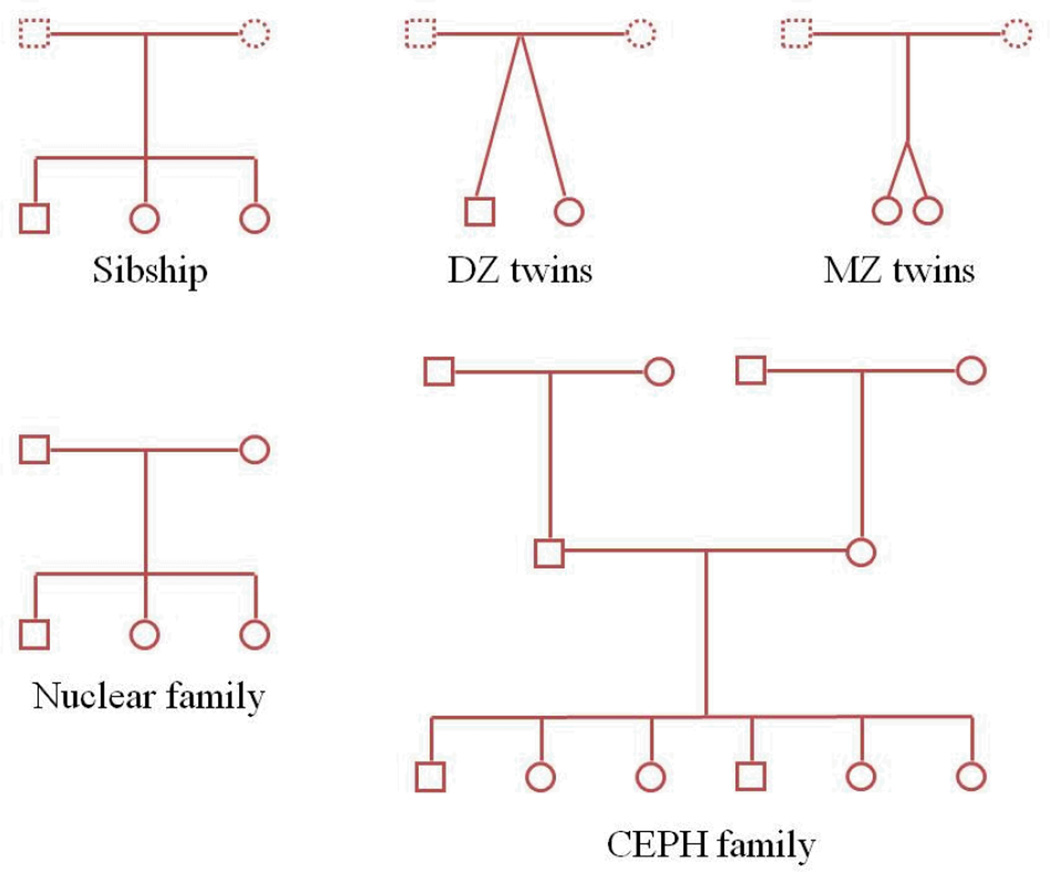
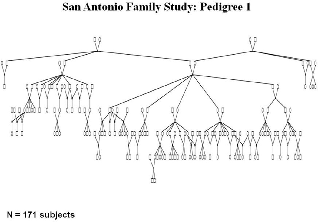
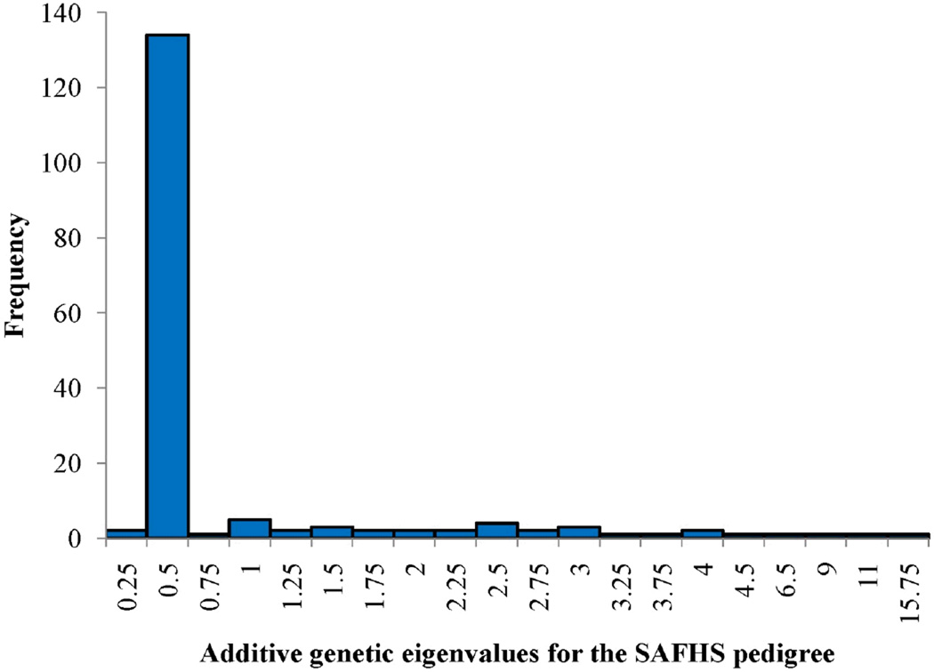
Our analytical results clearly demonstrate the primacy of the eigenvalues distribution for a given GRK as the focal determinant of power to detect heritability. For canonical relationships and simple pedigree structures such as those shown in Figure 3, the eigenvalues of the pedigree-derived GRK can be analytically determined. Such analytical determinations are extremely useful when considering theoretical issues of study design or when trying to determine what type of family would be best for recruitment in a given proposed study. Table 1 shows the analytical eigenvalues for those common pedigree structures depicted in Figure 3. For more complex extended families such as the one depicted in Figure 4 (this is an actual family from our San Antonio Family Heart Study (SAFHS) sample that has undergone WGS), the eigenvalues must be numerically determined by spectral decomposition of the pedigree-derived GRK. Figure 5 shows a histogram of the eigenvalues of the relationship matrix for this large pedigree that were obtained numerically. Recall that eigenvalues less than 1 contribute positively to the test statistic for heritability. As can be seen for relationship structures with more than two individuals in Table 1 and Figure 5, eigenvalues less than 1 are always more frequent. A slight problem arises for the case of monozygotic (MZ) twins in that the ELRT (and, in fact, the multivariate normal likelihood function) becomes degenerate at heritability exactly equal to 1. This problem can be dealt with by bounding the heritability slightly less than 1.

Figure 3.

Some simple relationship and pedigree structures.

Table 1.

Analytic eigenvalues for various relationship structures

Relationship structure	Additive genetic eigenvalues	ELRT per relationship unit
		h2 = 0.3	h2 = 0.7
MZ twins	2 0	0.09 (0.05)*	0.67 (0.34)
Sib pair	3/2 1/2	0.02 (0.005)	0.13 (0.03)
Sibship	(ns + 1)/2 (ns − 1){1/2}**	0.18 (0.04)#	0.85 (0.17)
Relative pair in GRK, K = {Kij}	1 + Kij 1 − Kij	0.006 (0.003)‡	0.03 (0.015)
Nuclear family	$(n_s+3)/4\pm \sqrt{2n_s+{(n_s-1)}^2/4}/2$ 1 (ns − 1){1/2}	0.17 (0.03)	0.90 (0.18)
CEPH family	(2){1} (ns){1/2} $1\pm \sqrt{2}/2$ $(n_s+4)/4\pm \sqrt{2(n_s+1)+{n_s}^2/4}/2$	0.56 (0.05)	2.54 (0.21)
Extended pedigree	Eigenvalues of K	10.30† (0.06)	40.62 (0.24)

^*The number in parentheses is the scaled individual contribution to the ELRT.

^**We use the symbology (x){y} to denote x units of value y. Otherwise, the operators are to be interpreted in the usual manner. For example, the first sibship entry means there is one eigenvalue at that value, and the second entry means that there are (n_s −1) eigenvalues (n_s being the number of sibs) each one equal to 1/2.

^#For 5 sibs.

^‡For grandparent-grandchild, or avuncular, or half-sib relationships.

^†For the extended pedigree in Figure 2 (N = 171).

Figure 4.

A San Antonio Family Heart Study (SAFHS) extended pedigree (N = 171 individuals).

Figure 5.

Numberically estimated eigenvalues of the SAFHS extended pedigree.

B. Power functions for heritability and association

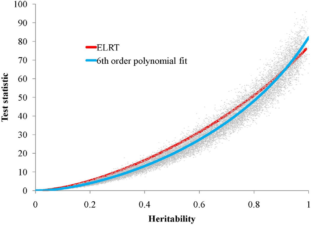
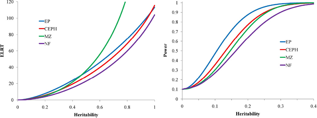
To evaluate the accuracy of the theory, we analyzed parametric bootstrap simulations of a quantitative trait sampled from the SAFS example pedigree. Basically, using the simulations modules in our SOLAR software (Almasy and Blangero, 1998), we simulated heritabilities across the parameter space and examined our empirical power to obtain significant evidence for genetic factors. Using 10,000 simulations including 10 copies of the SAFHS EP in each simulation, we obtained a close correspondence between theory and empirical observation. Figure 6 demonstrates how close the theoretical ELRTs come to a 6^th order polynomial fit of the simulated LRTs. Clearly, our very simple formula for the ELRT is suitably accurate for general use. Table 1 also shows the ELRT per relationship unit and per individual for two levels of heritability (0.30 and 0.70). Our results show a dependence of the ELRT upon the total heritability and the pedigree eigenvalues. Similarly, in Figure 7, we plot on the left panel the ELRTs for four of the different relationship structures, namely MZ twins (noted as MZ), nuclear families with three siblings (NF), CEPH-style families with six siblings (CEPH), and the SAFHS example pedigree (EP), all scaled to 250 individuals for easy comparison. In the right panel of Figure 7, we show the scaled power functions for heritability estimation for the same pedigree structures. Notably, the extended family design is most powerful in the region of the null. However, for heritabilities above approximately 0.47, the MZ design becomes most powerful. Our results indicate that the conventionally and widely held belief that monozygotic twins constitute the most powerful design for estimating heritability is not true in the most important part of the parameter space (i.e., in the local area of the null hypothesis).

Figure 6.

Parametric bootstrap of the LRT distribution. Simulation of 19,000 LRTs where the generating model is for heritability estimation using the SAFHS extended pedigree. 6^th order polynomial fit (blue line). ELRT computed for the SAFHS (red line).

Figure 7.

ELRT and power for heritability estimation. For both panels: SAFHS extended pedigree (EP) (blue line), CEPH-pedigree (red line), monozygotic twins (MZ) (green line), and nuclear family (NF) (purple line) all scaled to 250 individuals.

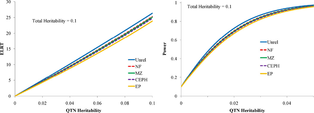
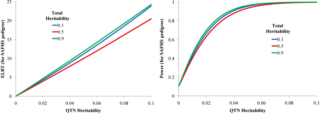
We examined similar study design comparisons in relation to association testing using Eq.(13). For a total heritability of 0.1, we plotted the association ELRTs for the four relationship structures, and power to detect association for the same fixed sample sizes in Figure 8. Figure 8 shows that for this fixed low total heritability and a reasonable range of QTN-specific heritabilities, power to detect associations is greatest in unrelated samples as expected. Loss of power is greatest in the extended pedigree due to the substantial correlation between subjects, however, even for this design the loss of power is low. Figure 9 shows the effect of total heritability on power to detect association for the extended pedigree. Power to detect association is influenced by total heritability with the power loss being maximized at a residual heritability of 0.50. Interestingly, power loss as seen in the ELRT is minimal both near the null region for heritability (as expected) and somewhat counter-intuitively near the maximum of heritability (at 1). Regardless, our theoretical results show little loss of power in the association analysis of even large and complex pedigrees. Furthermore, when considering the increased focus on the analysis of rare variants, power is actually substantially increased in large pedigrees due to the accumulation of multiple copies (and hence, increased genotypic variance) of rare variants incurred through Mendelian transmission in variant-harboring lineages.

Figure 8.

ELRT and power for association testing. For both panels: Unrelateds (blue line), nuclear family (NF) (red dashed line), monozygotic twins (MZ), (green line), CEPH pedigree (purple dashed line), and SAFHS extended pedigree (EP) (yellow).

Figure 9.

Effect of varying the total heritability on ELRT and power for association testing all scaled to 250 individuals. Total heritabilities equal to: 0.1 (blue line), 0.5 (red line), and 0.9 (green line).

C. Asymptotic Relative Efficiency

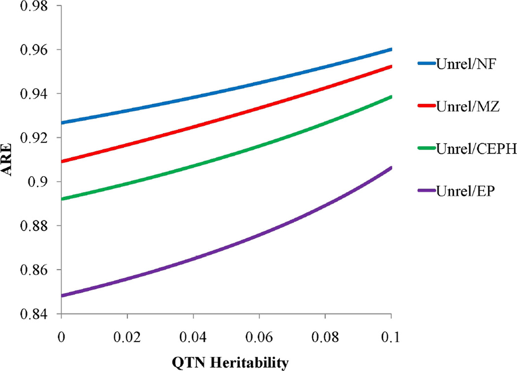
We also calculated the AREs for comparing peidgree-based designs for association analysis. Figure 10 shows all ARE comparisons relative to unrelateds in Figure 10, again scaled to 250 indviduals. Our results are consistent with those from a study by Visscher et al. (2008). They found that there is in fact little power loss on comparing the power to detect association in a sample of unrelateds versus in a sample of relatives. In fact, the power loss becomes even smaller at higher total heritabilities (analyses not shown) as suggested also in Figure 9.

Figure 10.

Pitman Asymptotic Relative Efficiency (ARE) for unrelated in relation to various family structures. Unrelateds in comparison to: nuclear family (NF) (blue line), monozygotic twins (MZ) (red line), CEPH family (green), and SAFHS extended pedigree (EP) (purple line).

D. Inadequacy of the Asymptotic LRT Distribution for Variance Component Testing

As we briefly discussed earlier, the asymptotic distribution of the LRT for testing the null hypothesis with regard to a variance component is given by a 50:50 mixture of ${\chi }_0^2$, which denotes a chi-square random variable with a point-mass at 0, and of ${\chi }_1^2$, a chi-square with 1 d.f. However, this is the appropriate distribution only if the data are i.i.d. (Crainiceanu et al., 2003, 2005; Crainiceanu and Ruppert, 2004a–c; Crainiceanu, 2008). Unfortunately, for most VC models in use in pedigree analyses including the ones under discussion here, this assumption is violated, and this departure has been shown to generate skewed mixture distributions that have an increased frequency of ${\chi }_0^2$ (i.e., an increased incidence of test statistics of zero). Researchers have found that the true frequency of ${\chi }_0^2$ can range from 0.65 to as high as 0.96(!) (Shephard and Harvey, 1990; Shephard, 1993; Kuo, 1999; Pinheiro and Bates, 2000; Crainiceanu et al., 2003; Crainiceanu et al., 2004a). This means that the traditional theory for non-standard cases can be severely conservative and hence show a loss of power. Consequently, Crainiceanu and colleagues developed an elegant and useful theory to recover the appropriate distribution (Crainiceanu et al., 2003, 2005; Crainiceanu and Ruppert, 2004a–c; Crainiceanu, 2008). In fact, like us, they also employ a spectral representation of the likelihood function to obtain a simplified LRT. Tailoring their theory to the present situation, let π_i and λ_gi be the eigenvalues of K^1/2PK^1/2 and K, respectively, where P = I − X(X′X)^{− 1} X′. For the heritability problem and large n, these two matrices (and their eigenvalues) tend towards equality. Then, if the true value of the heritability is given by $h_0^2$, their expression for the LRT is given as:

$$LRT=\underset{h^2}{\text{sup}}\left[n\text{ln}\right\{1+\frac{N}{D}\}-\sum \text{ln}(1+\frac{h^2{\lambda }_{gi}}{e^2}/1+\frac{h_0^2{\lambda }_{gi}}{e_0^2}\left)\right],$$ (19)

where e² =1 − h², $e_0^2=1-h_0^2,N=\sum \frac{{\pi }_i}{\psi }(h^2{e}_0^2-h_0^2{e}^2){\omega }_i^2,D=\sum \frac{e^2}{\mathrm{\psi }}(e_0^2+h_0^2{\mathrm{\pi }}_i){\mathrm{\omega }}_i^2+\sum _{i=1}^{n-j}{\mathrm{\omega }}_i^2,\psi =(e^2+h^2{\pi }_i)e_0^2$, the maximization is with regard to h², the summations are over all n values unless explicitly noted and the ω_i's are independent standard normal random variables, N (0,1) similar to the τ vector in Eq.(5). The probability of ${\chi }_0^2$ is equal to the probability that Eq. (19) has a global maximum at h² = 0. To approximate this probability, Crainiceanu and colleagues recommended computing the probability of a local maximum at h² = 0 for a given sample size. This probability is given as:

$$P\left\{\frac{\sum {\pi }_i{\omega }_i^2}{{\sum }_{i=1}^{n-j}{\omega }_i^2}\right\}\le \frac{1}{n}\sum {\lambda }_{gi}\Rightarrow P\left\{\frac{\sum {\pi }_i{\omega }_i^2}{{\sum }_{i=1}^{n-j}{\omega }_i^2}\right\}\le 1$$ (20)

Unfortunately, it appears that the true distribution of the LRT in finite situations is determined by the asymptotic distribution of the eigenvalues of the matrices involved. Thus, for every study and every covariate configuration, a separate LRT distribution should be examined. While this sounds formidable, these formulae suggest a simple and very rapid method for obtaining the true expected LRT distribution using simulation. We used the R program RLRsim (Scheipl et al., 2008; Scheipl and Bolker, 2012) to simulate the LRTs using the spectral representation of the LRT in Eq. (19) for our extended SAFHS pedigree (Figure 4). Fitting a mixture of a binomial and a ${\chi }_1^2$ distribution as suggested in Crainiceanu (2008) and Greven et al. (2008), we estimated a true mixing proportion of 0.57:0.43 and a multiplicative correction to the ${\chi }_1^2$ distribution of approximately 0.905. The true cut-off is closer to 2.3 than the asymptotic theory prediction of 2.7. Thus, as expected, reliance on the asymptotic theory for non-standard test cases will be conservative. Experimentation shows that there is much less of an effect on association inference and that the non-standard asymptotic theory holds well.

VI. ANALYSIS OF EMPIRICAL GRKs

Empirical GRKs have proven to be quite useful in the development of novel statistical genetic methods. Visscher and colleagues (Yang et al., 2011) have used empirical GRKs to even extract quantitative genetic information from “unrelated” individuals be exploiting deep ancestries. For example, one way to greatly reduce the problem of multiple hypothesis testing when analyzing a prohibitively large number of single nucleotide polymorphisms (SNPs) is to estimate K from the set of SNPs and to use it to model a variance component reflective of the aggregate effects of the SNPs (Wu et al., 2011). Obviously, the multiple testing problem is amplified in the setting of whole genome sequence data analysis, which accordingly increases the utility of a method that produces single degree of freedom tests. This approach has been applied to the analysis of several complex traits (Yang et al., 2010, 2011a), including height, body mass index, von Willebrand factor, and QT interval, and to schizophrenia (Lee et al., 2012). This idea could be extended to computing heritabilities on a chromosomal or a gene segment basis (Yang et al., 2011a). One could also leverage this approach to compute the K relevant for a metabolic pathway and to estimate pathway-specific variance components (Almeida et al., 2012). We have shown that it is possible to accurately recover both total and local (i.e., QTL-specific) heritability estimates by using only empirical GRKs in a known pedigree situation (Day-Williams et al, 2011). However, see Weir and Hill (2011) for cautionary caveats on the potential loss of accuracy in the empirical relatedness of remote relatives.

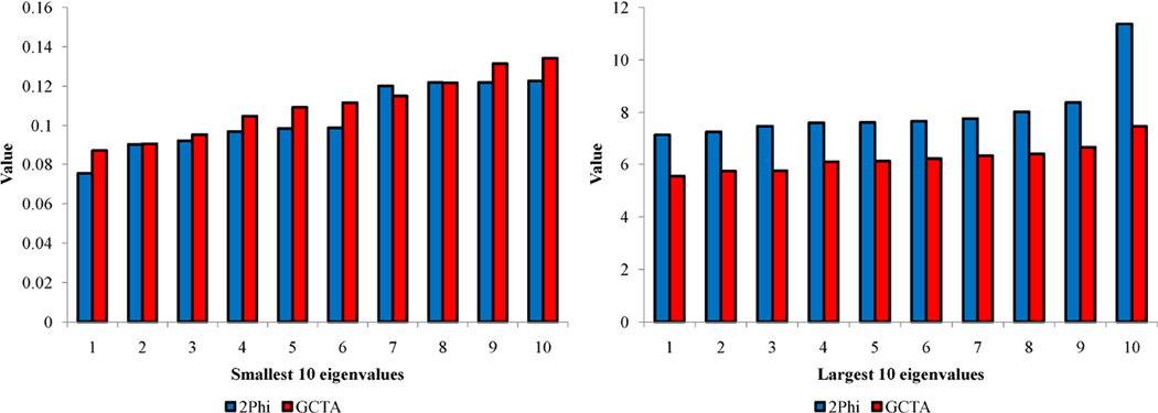
Empirical GRKs have the potential to make significant contributions to the statistical genetic analysis of complex traits and diseases. As an example of their use and to illustrate potential problems, we estimated a GRK using the GCTA software (Yang, Lee et al., 2011). Asymptotically, this procedure should yield a test of heritability that is consistent with that of the underlying average coefficient of relationship matrix. Again, we focused on the extended pedigrees of the general complexity as that shown in Fig. 4. We employed the WGS single nucleotide variant frequency spectrum information (for half the genome, specifically the odd-numbered autosomes)available on 20 SAFS pedigrees including 852 individuals with data utilized in the most recent Genetic Analysis Workshop 18 (Almasy et al., in press) that this pedigree was part of, and simulated 4.1M SNVs with minor allele frequencies > 0.01 for our GRK estimates. The resulting kernel is positive semi-definite (PSD). However, Fig. 11 shows that the critical eigenvalue distribution is different from that observed for the true pedigree-derived relationship matrix. Specifically, the GCTA leading eigenvalues are deflated which occurs when overall correlation amongst individuals is underestimated. Based on our Equation 7, this should lead to inflation of the test statistic. We performed a simulation experiment to test the influence of having an empirical GRK for heritability estimation. Using our SOLAR software, we obtained one million replicates under the null hypothesis of no heritability using the expected kernel given by the observed SAFHS pedigree structure. We then analyzed the simulated quantitative traits under the true generating model (using the pedigree-derived GRK) and under a model using the empirical GRK. We used the approach described in Equations (19) and (20) to obtain the true null distribution under the generating model. Using this cut-off, we observed that type 1 error for the GCTA GRK is inflated with a false positive rate of 0.053, a 6% increase in error. The type 1 error worsens to a 10% excess for a more stringent significance cutoff of 0.001.

Figure 11.

Comparison of the smallest and largest eigenvalues computed from the true pedigree-derived (2Phi) and GCTA relationship kernels. For both panels: 2Phi (blue columns), GCTA (red columns).

Whilst the GCTA GRK was PSD, many empirical GRK estimation procedures can lead to non-PSD kernels. Non-PSD matrices have been a bane in statistics in general and statistical genetics in particular for decades now. It was previously observed that a non-PSD covariance matrix can substantially bias heritability estimates (Hayes & Hill, 1980, 1981; Hill & Thompson, 1978). For non-PSD matrices, the larger eigenvalues are biased upward and the smaller eigenvalues are biased downward (Hayes & Hill, 1980, 1981; Hill & Thompson, 1978; Meyer & Kirkpatrick, 2008). Our ELRT formula (Equation 7) for heritability shows that negative eigenvalues will inflate the test statistic and hence may lead to increased type 1 error under the null hypothesis of no heritability. Because of the shape of the ln function, the negative eigenvalues have a disproportionate effect on the total test statistic. Our results suggest that it is important to constrain empirical GRKs to be PSD. This will typically require some type of post-processing of an estimated GRK. For example, an early approach was to correct such non-PSD matrices by adjusting the eigenvalue distribution so that the smallest eigenvalue equals 0 (Hayes & Hill, 1980, 1981; Kirkpatrick & Lofsvold, 1992). Subsequent approaches instead aimed to obtain a better estimate of the covariance matrix while guaranteeing the matrix to be PSD, and are reviewed in Meyer and Kirkpatrick (2008, 2010) and Meyer (2011). Our theoretical results suggest that care should be given when choosing empirical GRKs.

Discussion

The main theme of this work has been on the practical utility and unifying value of our eigensimplification of the polygenic VC likelihood function. The eigensimplification approach enables much more rapid computations that are equivalent to those required in samples of unrelateds after initial transformation, which is a highly practical benefit in this new era of high dimensional NGS data analysis. Importantly, it also led to elegant theoretical advances in regard to the ELRT, power analysis, and the analysis of GRKs. Our general formulae related to power to detect heritability in arbitrary pedigrees represents a solution to a difficult problem that has typically been handled using computer simulation. Our formulae unequivocally show that the critical parameters for power to detect heritability involve the eigenvalues of the pedigree-relationship matrix. We have also used our approach to examine the expected power of arbitrary pedigrees for detecting associations. Again, to assess power for association testing in pedigrees, investigators have typically been required to rely on cumbersome simulation strategies. Our formulae now allow rapid analytical evaluation of different study designs. Our simple formulation of the ELRT for association in pedigrees also shows exactly how power is lost due to non-independence between relatives. We also show that this power loss is relatively minor even for our largest most complex pedigree analyzed. Given that we are now entering an era where association studies of rare variants in large pedigrees is likely to rapidly increase, our results will be useful for aiding rational study design in the genetic dissection of complex phenotypes.

Our analytical approach is not without its own share of weaknesses. One major criticism that may turn out to be an inroad for future advance is that the exact spectral decomposition approach is limited to VC models with only two variance components. This is because only two kernels at a time can be simultaneously diagonalized whereas generalization to an arbitrary number of matrices requires numerical approximation (Flury and Gautschi, 1986). Thus, neither is the approach immediately able to incorporate a linkage variance component (certainly not analytically), which is known to greatly improve upon the overall VC statistical genetic model, nor is it possible to extend the approach to model genotype-by-environment interaction using an additional variance component. We are now working with empirical eigensimplification approaches which substantially reduce computation but not to the extent of that observed under the simple polygenic VC model, nor do they lead to such obvious insights into the canonical determinants of power. Notwithstanding these important criticisms, we believe that the eigensimplification approach of the classical additive polygenic model will lead to important empirical and possibly even additional theoretical discoveries.

Finally, all of the procedures discussed in this work have been (or will be in the near future) implemented into our general statistical genetic software package, SOLAR available from http://txbiomed.org/departments/genetics/genetics-detail?r=37.

References

- 1000 Genomes Project Consortium. Abecasis GR, Auton A, Brooks LD, DePristo MA, Durbin RM, Handsaker RE, Kang HM, Marth GT, McVean GA. An integrated map of genetic variation from 1,092 human genomes. Nature. 2012;491:56–65. doi: 10.1038/nature11632. [DOI] [PMC free article] [PubMed] [Google Scholar]
- Abadir KM, Magnus JR. Matrix Algebra. Cambridge: Cambridge University Press; 2005. [Google Scholar]
- Almasy L, Blangero J. Multipoint quantitative-trait linkage analysis in general pedigrees. Am. J. Hum. Genet. 1998;62:1198–1211. doi: 10.1086/301844. [DOI] [PMC free article] [PubMed] [Google Scholar]
- Almasy L, Blangero J. Variance component methods for analysis of complex phenotypes. 5. Vol. 2010. Cold Spring Harb Protoc; 2010. pdb.top77. [DOI] [PMC free article] [PubMed] [Google Scholar]
- Almasy L, Dyer TD, Peralta JM, Jun G, Fuchsberger C, Almeida MA, Kent JW, Jr, Fowler S, Duggirala R, Blangero J. Data for Genetic Analysis Workshop 18: Human Whole Genome Sequence, Blood Pressure, and Simulated Phenotypes in Extended Pedigrees. Genet. Epidemiol. doi: 10.1186/1753-6561-8-S1-S2. (In Press). [DOI] [PMC free article] [PubMed] [Google Scholar]
- Almeida M, Peralta J, Farook V, Puppala S, Duggirala R, Blangero J. Random Effect Burden Tests to Screen Gene Pathways. Genetic Analysis Workshop 18; October 13–17, 2012; Stevenson, WA. 2012. [Google Scholar]
- Anderson TW, Olkin I. Maximum-likelihood estimation of the parameters of a multivariate normal distribution. Lin. Alg. Appl. 1985;70:147–171. [Google Scholar]
- Bhattacharjee S, Wang Z, Ciampa J, Kraft P, Chanock S, Yu K, Chatterjee N. Using principal components of genetic variation for robust and powerful detection of gene-gene interactions in case-control and case-only studies. Am. J. Hum. Genet. 86:331–342. doi: 10.1016/j.ajhg.2010.01.026. [DOI] [PMC free article] [PubMed] [Google Scholar]
- Blangero J. Localization and identification of human quantitative trait loci: King Harvest has surely come. Curr. Op. Genet. Dev. 2004;14:233–240. doi: 10.1016/j.gde.2004.04.009. [DOI] [PubMed] [Google Scholar]
- Blangero J, Williams JT, Almasy L. Quantitative trait locus mapping using human pedigrees. Hum. Biol. 2000;72:35–62. [PubMed] [Google Scholar]
- Blangero J, Williams JT, Almasy L. Variance component methods for detecting complex trait loci. Advances in Genetics, v. 42. In: Rao DC, Province MA, editors. Genetic Dissection of Complex Traits. New York: Academic Press; 2001. pp. 151–181. [DOI] [PubMed] [Google Scholar]
- Blangero J, Göring HHH, Kent JW, Jr, Williams JT, Peterson CP, Almasy L, Dyer TD. Quantitative trait nucleotide analysis using Bayesian model selection. Hum Biol. 2005;77:541–559. doi: 10.1353/hub.2006.0003. [DOI] [PubMed] [Google Scholar]
- Boerwinkle E, Chakraborty R, Sing CF. The use of MG information in the analysis of quantitative phenotypes in man. I. Models and analytical methods. Ann. Hum. Genet. 1986;50:181–194. doi: 10.1111/j.1469-1809.1986.tb01037.x. [DOI] [PubMed] [Google Scholar]
- Boerwinkle E, Sing CF. The use of MG information in the analysis of quantitative phenotypes in man. III. Simultaneous estimation of the frequencies and effects of the apolipoprotein E polymorphism and residual polygenetic effects on cholesterol, betalipoprotein and triglyceride levels. Ann. Hum. Genet. 1987;51:211–226. doi: 10.1111/j.1469-1809.1987.tb00874.x. [DOI] [PubMed] [Google Scholar]
- Brown BW, Lovato J, Russell K. Asymptotic power calculations: description, examples, computer code. Stat Med. 1999;18(22):3137–3151. doi: 10.1002/(sici)1097-0258(19991130)18:22<3137::aid-sim239>3.0.co;2-o. [DOI] [PubMed] [Google Scholar]
- Chernoff H. On the distribution of the likelihood ratio. Ann. Math. Stat. 1954;25:573–578. [Google Scholar]
- Crainiceanu CM, Ruppert D, Vogelsang TJ. Some properties of the likelihood ratio tests in linear mixed models. 2003 Available at: http://legacy.orie.cornell.edu/davidr/papers/zeroprob_rev01.pdf. [Google Scholar]
- Crainiceanu CM, Ruppert D. Restricted likelihood ratio tests in nonparametric longitudinal models. Statistica Sinica. 2004a;14:713–729. [Google Scholar]
- Crainiceanu CM, Ruppert D. Likelihood ratio tests in linear mixed models with one variance component. J. R. Statist. Soc. B. 2004b;66:165–185. [Google Scholar]
- Crainiceanu CM, Ruppert D. Likelihood ratio tests for goodness-of-fit of a nonlinear regression model. J. Multivar. Anal. 2004c;91:35–52. [Google Scholar]
- Crainiceanu CM, Ruppert D, Claeskens G, Wand MP. Exact likelihood ratio tests for penalized splines. Biometrika. 2005;92:91–103. [Google Scholar]
- Crainiceanu CM. Likelihood ratio testing for zero variance components in linear mixed models. In: Dunson DB, editor. Random Effect and Latent Variable Model Selection. New York: Springer; 2008. pp. 3–17. [Google Scholar]
- DasGupta A. Asymptotic Theory of Statistics and Probability. New York: Springer; 2008. [Google Scholar]
- Day-Williams AG, Blangero J, Dyer TD, Lange K, Sobel EM. Linkage analysis without defined pedigrees. Genet Epidemiol. 2011;35:360–370. doi: 10.1002/gepi.20584. [DOI] [PMC free article] [PubMed] [Google Scholar]
- Dempster AP, Patel CM, Selwyn MR, Roth AJ. Statistical and computational aspects of mixed model analysis. Appl. Stat. 1985;33:203–214. [Google Scholar]
- Dominicus A, Skrondal A, Gjessing HK, Pedersen NL, Palmgren J. Likelihood ratio tests in behavioral genetics: Problems and solutions. Behav. Genet. 2006;36:331–340. doi: 10.1007/s10519-005-9034-7. [DOI] [PubMed] [Google Scholar]
- Dyer TD, Diego VP, Kent JW, Jr, Göring HHH, Blanger J. Rapid exact likelihood-based quantitative trait association analysis in large pedigrees. American Society of Human Genetics Annual Meeting; October 20–24, 2009; Honolulu, HI. 2009. [Google Scholar]
- Fisher RA. The correlation between relatives on the supposition of Mendelian inheritance. Trans. R. Soc. Edinburgh. 1918;52:399–433. [Google Scholar]
- Flury BN, Gautschi W. An algorithm for simultaneous orthogonal transformation of several positive definite symmetric matrices to nearly diagonal form. S.I.A.M. J. Sci. Stat. Comput. 1986;7:167–184. [Google Scholar]
- Giampaoli V, Singer JM. Likelihood ratio tests for variance components in linear mixed models. J. Statist. Plan. and Infer. 2009;139:1435–1448. [Google Scholar]
- Greven S, Crainiceanu CM, Küchenhoff H, Peters A. Restricted likelihood ratio testing for zero variance components in linear mixed models. J. Comput. Graph. Stat. 2008;17:870–891. [Google Scholar]
- Hayes JF, Hill WG. A reparameterization of a genetic selection index to locate its sampling properties. Biometrics. 1980;36:237–248. [PubMed] [Google Scholar]
- Hayes JF, Hill WG. Modification of estimates of parameters in the construction of genetic selection indices ('bending') Biometrics. 1981;37:483–493. [Google Scholar]
- Hill WG, Thompson R. Probabilities of non-positive definite between-group or genetic covariance matrices. Biometrics. 1978;34:429–439. [Google Scholar]
- Hill WG, Weir BS. Variation in actual relationship as a consequence of Mendelian sampling and linkage. Genet. Res. 2011;93:47–64. doi: 10.1017/S0016672310000480. [DOI] [PMC free article] [PubMed] [Google Scholar]
- Hopper JL, Matthews JD. Extensions to multivariate normal models for pedigree analysis. Ann. Hum. Genet. 1982;46:373–383. doi: 10.1111/j.1469-1809.1982.tb01588.x. [DOI] [PubMed] [Google Scholar]
- Kang HM, Sul JH, Service SK, Zaitlen NA, Kong SY, Freimer NB, Sabatti C, Eskin E. Variance component model to account for sample structure in genome-wide association studies. Nat Genet. 2010;42:348–354. doi: 10.1038/ng.548. [DOI] [PMC free article] [PubMed] [Google Scholar]
- Kang HM, Zaitlen NA, Wade CM, Kirby A, Heckerman D, Daly MJ, Eskin E. Efficient control of population structure in model organism association mapping. Genetics. 2008;178:1709–1723. doi: 10.1534/genetics.107.080101. [DOI] [PMC free article] [PubMed] [Google Scholar]
- Kim W, Gordon D, Sebat J, Ye KQ, Finch SJ. Computing power and sample size for case-control association studies with copy number polymorphism: Application of mixture-based likelihood ratio test. PLoS One. 2008;3:e3475. doi: 10.1371/journal.pone.0003475. [DOI] [PMC free article] [PubMed] [Google Scholar]
- Kirkpatrick M, Lofsvold D. Measuring Selection and Constraint in the Evolution of Growth. Evolution. 1992;46:954–971. doi: 10.1111/j.1558-5646.1992.tb00612.x. [DOI] [PubMed] [Google Scholar]
- Kuo B-S. Asymptotics of ML estimator for regression models with a stochastic trend component. Econometr. Theor. 1999;15:24–49. [Google Scholar]
- Lange K. Mathematical and Statistical Methods for Genetic Analysis. 2nd ed. New York: Springer-Verlag; 2002. [Google Scholar]
- Lee SH, DeCandia TR, Ripke S, Yang J. Schizophrenia Psychiatric Genome-Wide Association Study Consortium (PGC-SCZ); International Schizophrenia Consortium (ISC); Molecular Genetics of Schizophrenia Collaboration (MGS) Estimating the proportion of variation in susceptibility to schizophrenia captured by common SNPs. In: Sullivan PF, Goddard ME, Keller MC, Visscher PM, Wray NR, editors. Nat. Genet. Vol. 44. 2012. pp. 247–250. [DOI] [PMC free article] [PubMed] [Google Scholar]
- Liu B. Statistical Genomics: Linkage, Mapping, and QTL Analysis. Boca Raton: CRC Press; 1999. [Google Scholar]
- Meyer K. Performance of penalized maximum likelihood in estimation of genetic covariances matrices. Genet. Sel. Evol. 2011;43:39. doi: 10.1186/1297-9686-43-39. [DOI] [PMC free article] [PubMed] [Google Scholar]
- Meyer K, Kirkpatrick M. Perils of parsimony: properties of reduced-rank estimates of genetic covariance matrices. Genetics. 2008;180:1153–1166. doi: 10.1534/genetics.108.090159. [DOI] [PMC free article] [PubMed] [Google Scholar]
- Meyer K, Kirkpatrick M. Better estimates of genetic covariance matrices by "bending" using penalized maximum likelihood. Genetics. 2010;185:1097–1110. doi: 10.1534/genetics.109.113381. [DOI] [PMC free article] [PubMed] [Google Scholar]
- Miller JJ. Asymptotic properties of maximum likelihood estimates in the mixed model of the analysis of variance. Ann. Stat. 1977;5:746–762. [Google Scholar]
- Moll PP, Powsner R, Sing CF. Analysis of genetics and environmental sources of variation in serum cholesterol in Tecumseh, Michigan V. Variance components estimated from pedigrees. Ann. Hum. Genet. 1979;42:343–354. doi: 10.1111/j.1469-1809.1979.tb00668.x. [DOI] [PubMed] [Google Scholar]
- Noether GE. Asymptotic properties of the Wald-Wolfowitz test of randomness. Ann. Math. Stat. 1950;21:231–246. [Google Scholar]
- Noether GE. On a theorem of Pitman. Ann. Math. Stat. 1955;26:64–68. [Google Scholar]
- Ott J, Kamatani Y, Lathrop M. Family-based designs for genome-wide association studies. Nat. Rev. Genet. 2011;12:465–474. doi: 10.1038/nrg2989. [DOI] [PubMed] [Google Scholar]
- Patterson HD, Thompson R. Recovery of inter-block information when block sizes are unequal. Biometrika. 1971;58:545–554. [Google Scholar]
- Pettofrezzo AJ. Matrices and Transformations. New York: Dover Publications; 1978. [Google Scholar]
- Pinheiro JC, Bates DM. Mixed-Effects Models in S and S-Plus. New York: Springer; 2000. [Google Scholar]
- Rijsdijk FV, Hewitt JK, Sham PC. Analytic power calculation for QTL linkage analysis of small pedigrees. Eur. J. Hum. Genet. 2001;9:335–340. doi: 10.1038/sj.ejhg.5200634. [DOI] [PubMed] [Google Scholar]
- Scheipl F, Greven S, Küchenhoff H. Size and power of tests for zero random effect variance or polynomial regression in additive and linear mixed models. Comput. Stat. Data Anal. 2008;52:3283–3299. [Google Scholar]
- Scheipl F, Bolker B. Package 'RLRsim'. 2012 Available at: http://cran.r-project.org/web/packages/RLRsim/index.html. [Google Scholar]
- Self SG, Liang K-Y. Asymptotic properties of maximum likelihood estimators and likelihood ratio tests under nonstandard conditions. J. Am. Statist. Assoc. 1987;82:605–610. [Google Scholar]
- Self SG, Mauritsen RH, Ohara J. Power calculations for likelihood ratio tests in generalized linear models biometrics. 1992;48:31–39. doi: 10.1111/j.0006-341x.2000.01192.x. [DOI] [PubMed] [Google Scholar]
- Sham PC, Cherny SS, Purcell S, Hewitt JK. Power of linkage versus association analysis of quantitative traits, by use of variance-components models, for sibship data. Am. J. Hum. Genet. 2000;66:1616–1630. doi: 10.1086/302891. Erratum in: Am. J. Hum. Genet., 2000, 66: 2020. [DOI] [PMC free article] [PubMed] [Google Scholar]
- Sham PC, Purcell S, Cherny SS, Abecasis GR. Powerful regression-based quantitative-trait linkage analysis of general pedigrees. Am. J. Hum. Genet. 2002;71:238–253. doi: 10.1086/341560. [DOI] [PMC free article] [PubMed] [Google Scholar]
- Shephard NG, Harvey AC. On the probability of estimating a deterministic component in the local level model. J. Time Series Anal. 1990;11:339–347. [Google Scholar]
- Shephard N. Maximum likelihood estimation of regression models with stochastic trend components. J. Am. Statist. Assoc. 1993;88:590–595. [Google Scholar]
- Stram DO, Lee JW. Variance components testing in the longitudinal mixed effects model. Biometrics. 1994;50:1171–1177. [PubMed] [Google Scholar]
- Stuart A, Ord JK. Kendall’s Advanced Theory of Statistics. Volume 1. Distribution Theory. 5th ed. New York: Oxford University Press; 1987. [Google Scholar]
- Thompson EA, Shaw RG. Pedigree analysis for quantitative traits: Variance components without matrix inversion. Biometrics. 1990;46:399–413. [PubMed] [Google Scholar]
- Thompson EA, Shaw RG. Estimating polygenic models for multivariate data on large pedigrees. Genetics. 1992;131:971–978. doi: 10.1093/genetics/131.4.971. [DOI] [PMC free article] [PubMed] [Google Scholar]
- Thompson R. The estimation of variance and covariance components with an application when records are subject to culling. Biometrics. 1973;29:527–550. [Google Scholar]
- Thompson R. Estimation of quantitative genetic parameters. Proc. R. Soc. Lond., Biol. Sci. 2008;275:679–686. doi: 10.1098/rspb.2007.1417. [DOI] [PMC free article] [PubMed] [Google Scholar]
- Thompson R, Cameron ND. Estimation of genetic parameters. 3rd World Congress on Genetics Applied to Livestock Production; University of Nebraska, Institute of Agriculture and Natural Resources; July 16-22, 1986; Lincoln. 1986. pp. 371–381. Lincoln, Neb. [Google Scholar]
- Thompson R, Meyer K. Estimation of variance components: What is missing in the EM algorithm? J. Statist. Comput. Simul. 1986;24:215–230. [Google Scholar]
- Verbeke G, Molenberghs G. The use of score tests for inference on variance components. Biometrics. 2003;59:254–262. doi: 10.1111/1541-0420.00032. [DOI] [PubMed] [Google Scholar]
- Visscher PM. A note on the asymptotic distribution of likelihood ratio tests to test variance components. Twin Res. Hum. Genet. 2006;9:490–495. doi: 10.1375/183242706778024928. [DOI] [PubMed] [Google Scholar]
- Visscher PM, Duffy DL. The value of relatives with phenotypes but missing genotypes in association studies for quantitative traits. Genet Epidemiol. 2007;30:30–36. doi: 10.1002/gepi.20124. Erratum in: Genet Epidemiol., 2007, 31, 801. [DOI] [PubMed] [Google Scholar]
- Visscher PM, Andrew T, Nyholt DR. Genome-wide association studies of quantitative traits with related individuals: Little (power) lost but much to be gained. Eur J Hum Genet. 2008;16:387–390. doi: 10.1038/sj.ejhg.5201990. [DOI] [PubMed] [Google Scholar]
- Wald A. Tests of statistical hypotheses concerning several parameters when the number of observations is large. Trans. Am. Mathemat. Soc. 1943;54:426–482. [Google Scholar]
- Williams JT, Blangero J. Power of variance component linkage analysis to detect quantitative trait loci. Ann. Hum. Genet. 1999a;63:545–563. doi: 10.1017/S0003480099007848. [DOI] [PubMed] [Google Scholar]
- Williams JT, Blangero J. Asymptotic power of likelihood ratio tests for detecting quantitative trait loci using the COGA data. Genet. Epidemiol. 1999b;17:S397–S3402. doi: 10.1002/gepi.1370170767. [DOI] [PubMed] [Google Scholar]
- Wu MC, Lee S, Cai T, Li Y, Boehnke M, Lin X. Rare-variant association testing for sequencing data with the sequence kernel association test. Am. J. Hum. Genet. 2011;89:82–93. doi: 10.1016/j.ajhg.2011.05.029. [DOI] [PMC free article] [PubMed] [Google Scholar]
- Yang J, Wray NR, Visscher PM. Comparing apples and oranges: equating the power of case-control and quantitative trait association studies. Genet Epidemiol. 2010;34:254–257. doi: 10.1002/gepi.20456. [DOI] [PubMed] [Google Scholar]
- Yang J, Manolio TA, Pasquale LR, Boerwinkle E, Caporaso N, Cunningham JM, de Andrade M, Feenstra B, Feingold E, et al. Genome partitioning of genetic variation for complex traits using common SNPs. Nat Genet. 2011;43:519–525. doi: 10.1038/ng.823. [DOI] [PMC free article] [PubMed] [Google Scholar]
- Yang J, Lee SH, Goddard ME, Visscher PM. GCTA: a tool for genome-wide complex trait analysis. Am. J. Hum. Genet. 2011;88:76–82. doi: 10.1016/j.ajhg.2010.11.011. [DOI] [PMC free article] [PubMed] [Google Scholar]
- Yang J, Benyamin B, McEvoy BP, Gordon S, Henders AK, Nyholt DR, Madden PA, Heath AC, Martin NG, Montgomery GW, et al. Common SNPs explain a large proportion of the heritability for human height. Nat Genet. 2010;42:565–569. doi: 10.1038/ng.608. [DOI] [PMC free article] [PubMed] [Google Scholar]