Using the power balance model to simulate cross-country skiing on varying terrain

Abstract

The current study adapts the power balance model to simulate cross-country skiing on varying terrain. We assumed that the skier’s locomotive power at a self-chosen pace is a function of speed, which is impacted by friction, incline, air drag, and mass. An elite male skier’s position along the track during ski skating was simulated and compared with his experimental data. As input values in the model, air drag and friction were estimated from the literature based on the skier’s mass, snow conditions, and speed. We regard the fit as good, since the difference in racing time between simulations and measurements was 2 seconds of the 815 seconds racing time, with acceptable fit both in uphill and downhill terrain. Using this model, we estimated the influence of changes in various factors such as air drag, friction, and body mass on performance. In conclusion, the power balance model with locomotive power as a function of speed was found to be a valid tool for analyzing performance in cross-country skiing.

Introduction

Humans have devised various tools (eg, skis, skates, and snowshoes) to move more easily and fast across surfaces covered by snow or ice, and Scandinavians have been using skis for travel and transport across snow-covered terrain for over 4,000 years. Due to the effectiveness of skiing, it evolved into a competitive sport, and a 5 km race in Tromsø, in Northern Norway, on March 30, 1843, is considered to be the world’s first official cross-country skiing competition. Since the first Winter Games in Chamonix, France, in 1924, cross-country skiing has been an Olympic event, with competitions performed on varying terrain and at widely varying speeds. In such terrain, a skier must constantly alter his technique and locomotive power according to the incline, snow friction, and air drag,1–3 and elite cross-country skiers are found to produce higher locomotive power and use higher exercise intensities (ie, metabolic rate) on uphill compared with flatter terrain.2,4,5 However, a skier’s locomotive power not only correlates with incline, but with technique and metabolic rate.4,6,7 Since these factors are all influenced by a skier’s speed, we assumed that the skier’s locomotive power during self-paced skiing in varying terrain could be simulated as a function of speed.

The power balance equation relates power production and power dissipation, enables more thorough scrutinization of how various factors interact in influencing endurance performance, and has been shown to be successful for predicting performance in running, cycling, and speed skating.8–10 Recently, power balance equations have been used on cross-country skiing.5,6,11,12 In a numerical simulation by Carlsson et al,13 the authors accounted for gravitational force, normal force between snow and skis, drag force from the wind, frictional force between snow and ski, and propulsive force. A further development was done by Sundstrøm et al,12 who developed an optimization process of locomotive power. A locomotive power function, described as a function of speed, was used as a constraint, together with a constraint in the average locomotive power during the race. However, the outcomes were not compared with experimental results. The aim of our paper, therefore, was to adapt the power balance model to simulate cross-country skiing performance on varying terrain and compare simulated with experimental results. We hypothesized that a skier’s position and time at each position along the track during a race could be accurately simulated by a power balance model, where the skier’s locomotive power is a function of speed.

Methods

Overall design

The current study adapted a power balance model to simulate cross-country skiing at a self-chosen pace in varying terrain. The skier’s locomotive power was assumed to be a function of speed. Thereafter, a skier’s simulated position along the track during ski skating was compared with experimental data. Using this model, we estimated the influence of changes in various factors such as air drag, friction, and body mass on performance. As input values, air drag and friction were estimated from the literature. The simulations were performed in Mathematica 9 (Wolfram Research Inc., Champaign, IL, USA). Before providing the written consent to participate, the subject was fully informed of the nature of the study, which was preapproved by the Norwegian Regional Ethics Committee.

Power balance equation

A skier’s rate of change in kinetic energy (E_k) equals body mass (m) multiplied by speed (v) of the center of mass of the skier and acceleration (dv/dt), where t is time. The locomotive power (P) is exclusively the power that generates locomotion. The power balance equation11,14 states that:

$$\begin{array}{l}\underset{\begin{array}{l}\mathit{\text{Rate of change of kinetic energy of skier}}\end{array}}{\underbrace{d\left(E_{\mathrm{k}}\right)/dt}}=mv\frac{dv}{dt}\\ =\underset{\begin{array}{l}\mathit{\text{Locomotive power}}\end{array}}{\underbrace{P}}-\underset{\begin{array}{l}\mathit{\text{Friction power}}\end{array}}{\underbrace{\mu F_{\mathrm{N}}v}}-\underset{\begin{array}{l}\mathit{\text{Gravitational power}}\end{array}}{\underbrace{mgSin\left(\alpha \right)v}}-\underset{\begin{array}{l}\mathit{\text{Air drag power}}\end{array}}{\underbrace{\frac{1}{2}\rho C_{\mathrm{d}}A{v}^3}}\end{array}$$ (1)

where μ is the friction coefficient, g is the gravitational acceleration, ρ is the air density, C_d is the drag coefficient, A is the projected front area of the skier (m²), m is the body mass, and α is the angle of inclination measured in radians between a tangent of the track and the horizontal level. Tan(α) = dh(s)/dx, Sin(α) = dh(s)/ds, where h(s) is the height of the terrain relative to the starting point, as a function of the accumulated distance s along the terrain from the beginning of the track, and x is the horizontal position. With this geometry, α=π/4=0.79 corresponds with 45°, and α=π/2 corresponds with vertical. We used straight lines between points, which means a piecewise linear track. For the relatively small angles of inclination used in the current study, Tan (α) ≈ Sin (α) ≈ α. F_N is the normal force on the terrain and is given as F_N = mgCos (α)−mv²/R, where R is the radius of curvature of the track. However, in this study we only use a track that is piecewise linear, and this term is thus set to zero. All parameters are positive; α has a maximum value of π/2, and the parameters μ, ρ, C_d, and m can have arbitrarily high values and be functions of time. The parameters α, μ, ρ, C_d, and m can change continuously and abruptly, but not discontinuously. This allows us to solve the differential equation in Equation 1.

Comparing simulated cross-country skiing with experimental data

By using the power balance model, 4,218 m cross-country skiing at a self-chosen pace on varying terrain was simulated for a skier with a mass of 77.5 kg. The track profile is shown in Figure 1, where the 13 filled squares are the points where time measurements were made for the skier along the track, and the 50 stars are the height measurement points. A straight line was drawn between each star. The blue curve is the track profile when fitting the 50 height measurements to a cubic spline function tabulated as piecewise linear. The model was solved for each straight line. As input to the power balance model, air drag and friction were estimated from the literature. Research assistants measured time by synchronized stopwatches when the skier passed the defined points along the track. An inverse relationship exists between time and distance, so that time measured as a function of distance can be used in a model where distance is a function of time. We did not perform any repeated measures of performance for this skier, which might be regarded a weakness of the current design. However, ski results from national and international sprint competitions, as well as performance tests in our laboratory indicate that elite skiers, like the skier in our study, are able to reproduce performance by a standard deviation of less than 2%.

Figure 1.

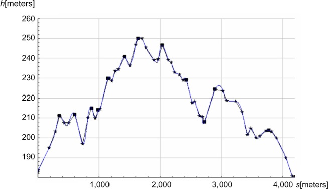
The height (h) in the terrain as a function of accumulated distance (s).

Notes: Straight lines are drawn between each star, which means a piecewise linear track; ■ denotes 13 points where time measurements were made; blue curve is a cubic spline fit.

The racing terrain was described by height (h) in meters as a function of distance (s) in meters along the terrain and used as input to the simulations. A constant friction coefficient μ of 0.037 was applied. This friction coefficient was based on findings for snow conditions similar to the test day, with old grained snow and −2°C. Air drag depends on the posture of the skier, which can be upright, semi-squatting, or deep tuck. Leirdal et al15 estimated C_dA =0.45 m² in upright posture, and C_dA =0.39 m² in semi-squatting posture. Spring et al16 reported C_dA values of 0.6 for upright posture and 0.3 in a deep-tuck posture. The deep-tuck posture incurs a metabolic cost but no locomotive power (since no propulsive force is generated). Here, we assumed that when the speed is higher than 10 m/second, the skier mainly uses the deep-tuck posture, and we set C_dA =0.35 m² when and C_dA =0.55 m² the speed was ≤10 m/second and an upright posture was employed. The air density (ρ) was 1.29 g/cm³.

Equation 1 can be divided by v. This gives the motion equations of the skier’s center of mass as:

$$\begin{array}{l}m\frac{dv}{dt}=P/v(t)-\mu mg\sqrt{1-h\prime {(s(t))}^2}-mgh\prime (s(t))-\frac{1}{2}\rho C_{\mathrm{d}}A{\left(V+v(t)\right)}^2\mathit{\text{Sign}}[V+v(t)],\\ \frac{ds}{dt}=v(t),\mathit{\text{Sign}}[V+v(t)]=\{\begin{array}{l}1\text{when}V+v(t)>0\hfill \\ -1\text{when}V+v(t)<0\hfill \\ 0\text{when}V+v(t)=0\hfill \end{array}\end{array}$$ (2)

where V is the wind speed in m/second, which is negative for tailwind and positive for headwind. The equations in Equation 2 were solved numerically, as two coupled nonlinear ordinary differential equations, to find the accumulated distance s(t) from the beginning of the track and the speed v(t) of the skier as a function of time; s(t) and h(s(t)) were compared with experimental results.

In the literature, a cross-country skier’s physiological response to different work rates has been repeatedly studied.4,7,8 However, no study to date has provided a model that predicts how the skier’s locomotive power P depends on the variety of factors involved when skiing outdoors. The skier’s locomotive power P can be optimized for minimum racing time applying various constraints. Sundstrøm et al12 used a given locomotion as a function of speed as a constraint together with constraint in the average locomotive power during the race. However, it may be questioned whether the constraint for average locomotive power may be reformulated to include the increased accumulation of fatigue. In this present study, we chose a different method: we assumed that the chosen P is a function of the skier’s speed, specific for each skier, where speed, in turn, depends on other factors. That is, through v, P depends indirectly on the angle of incline,4,7,8,13 friction, air drag, and the skier’s pace. It can be hypothesized that for typical racing speeds, locomotive power P decreases with increasing speed at a given intensity (note that the higher speeds are used at lower inclines). Various tests done for this paper and the findings of Sandbakk et al6 show that for speeds below 6 m/second, the locomotive power for a given metabolic energy decreases only marginally with increasing speed, while for racing speed above 6 m/second, locomotive power significantly decreases with increasing speed. However, the exact functional form of P(v) is unknown in the literature. Skiers may generate locomotive power above 10 m/second, but Andersson et al17 showed that skiers prefer to use techniques where they save their energy for the flat and uphill parts rather than producing work downhill at high speeds. Thus, skiers usually use the deep-tuck posture for speeds above 10 m/second. The dependence of P on α through v means that in steep uphill terrain, with high α, speed (v) is low, and locomotive power (P) is high. We here studied three functional forms for P(v) that each depends on two parameters determined by two optimization methods. These are exponential decrease, nonlinear decrease, and the inverse logistic function, ie:

$$\begin{array}{l}\text{Model}1:P(v)=P_{\max }Exp\left(-{(v/b)}^n\right)\\ \text{Model}2:P(v)=P_{\max }Max[0,1-{(v/b)}^n]\\ \text{Model}3:P(v)=P_{\max }\left(1-\frac{1}{1+Exp(a/b)Exp(-v/b)}\right)\end{array}$$ (3)

Figure 2 shows the locomotive power (P) as a function of speed (v) for the three models, with various parameter values. Here, for comparison, we also show the model by Sundstrøm et al.12 First, we minimized the summed square difference between the experimental distance and simulated distance at the measured time for the 12 track lengths considered separately. Second, we minimized the summed square difference between the experimental and simulated average speed for the 12 track lengths considered separately. The time was restarted at each subsequent experimental position datapoint. The experimental time and simulated time until the next experimental position was determined. The average experimental speed between these two experimental position datapoints is the experimental distance divided by the experimental time. The average simulated speed between the two points is the experimental distance divided by the simulated time. The maximum metabolic rate of the skier was assumed to be 1,890 J/second, and the gross efficiency for an uphill incline was around 0.155, based on treadmill roller ski testing of this skier. The lactate threshold for this skier was a fraction (0.88) of the maximum metabolic rate. Based on experience, the skier may use a mean metabolic rate approximately 5%–10% above the lactate threshold in uphill parts of a 4,218 m competition, ie, 1,746–1,830 J/second. Applying a visual curve fitting exercise, we used 7% above the lactate threshold as baseline, ie, 1,780 J/second. Multiplying the latter with 0.155 gives P_max =275 J/second, which we set as the maximum of P. To find the speed dependency of P(v), we used the inductive–deductive method. The P(v) was the induction. The simulated position versus time was the deduction, which was compared with the experimental data. Thus, P(v) is specific for each skier under the same fitness.

Figure 2.

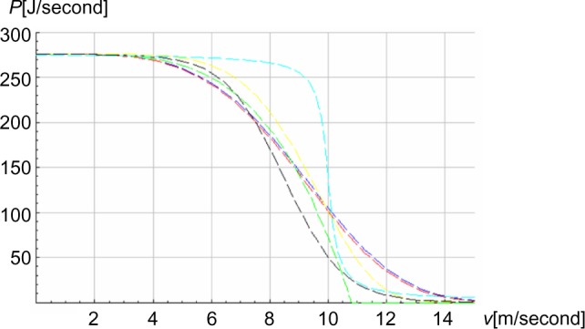
The locomotive power (P) as a function of speed (v) for the three models for various parameter values.

Notes: Blue, model 1 (n=4, b=10.1 m/s); red, model 1 (n=4, b=10.0 m/s); yellow, model 1 (n=6, b=10.0 m/s); green: model 2 (n=4, b=10.8 m/s); black, model 3 (a=8.5 m/s, b=1.0 m/s); cyan, function from Sundstrøm et al12 scaled vertically to reach maximum P_max=275 when v=0.

Methodological basis for sensitivity analysis

In this section, we discuss realistic lower and upper limits for the six parameters m, μ, ρ, V, P_max, and C_dA to test in a sensitivity analysis. First, we set that the mass of an elite skier can vary ±15 kg from baseline. Variation above this may change the technique of and therefore the locomotive power (P) in Figure 2 directly. Second, friction depends on mass, temperature, and velocity. During very wet or very cold conditions, it can be as low as 0.01, but 0.06 is probably maximum during racing conditions. Here, we vary between 0.03 and 0.06. Third, the density depends strongly on temperature and height above sea level. Assuming a temperature of +10°C at 2,000 m height and standard atmospheric pressure of 1,013 mb, at sea level, the pressure is 800 mb and the density is 0.98 g/cm³ at 2,000 m according to the barometric height formula. However, assuming a low pressure of 960 mb at sea level, the standard atmospheric pressure is 758 mb and the density is 0.93 g/cm³ at 2,000 m above sea level. Assuming −15°C at sea level and standard atmospheric pressure of 1,013 mb, the density is 1.37 g/cm³. However, assuming a high pressure of 1,030 mb, the density is 1.39 g/cm³. We set that the density can vary from 0.9 to 1.4 g/cm³ as the maximum range. Fourth, wind speed can vary substantially, but we considered the range from −5 to +5 m/second. Fifth, regarding the maximum locomotive power, the skier is not always in optimum fitness. How fitness development of a skier influences the locomotive function is unknown. Thus, varying the P_max parameter in Equation 3 may be relevant. We varied P_max by a factor of 0.8–1.2 for our skier, and model the locomotive power when the skier performs his best in a race. This model does not account for a skier racing less than 100%, for example to save energy for the last part of the race. Racing less than 100% means to choose locomotive power P(v) distinctly lower than that expressed in Equation 3 and shown in Figure 2. In such cases, the skier chooses lower rather than higher P(v) for a lower speed (v) to save energy. Sixth, as mentioned above, uncertainties in C_dA often exist, according to the literature (eg, Spring et al16), and pacing behind other skiers can also reduce the drag. We set that the C_dA function can vary by a factor of 0–1.5. C_dA =0 corresponds to treadmill conditions without any drag. We let the wind speed vary from V =−5 to +5 m/second.

Results

Figure 1 shows the track profile. Table 1 shows the root of the summed squared difference for Models 1 and 2 using the two optimization methods to determine the optimal integer values of the parameters n and b in Equation 3. Allowing one decimal place in the parameters, for the first method (distance difference), the optimal values were (n, b, r) = (4.0, 10.1 m/second, 171), (n, b, r) = (4.0, 10.8 m/second, 168), and (a, b, r) = (8.5 m/second, 1.0 m/second,169) for models 1, 2, and 3, respectively, where r is the root of the summed square difference. For the second method (speed difference) the optimal values were (n, b, r) = (4.0, 10.1 m/second, 2.81), (n, b, r) = (4.0, 10.8 m/second, 2.81), (a, b, r) = (8.5 m/second, 1.0 m/second, 2.81) for models 1, 2, and 3, respectively. Due to the uncertainty in the track profile, time measurements, coefficient of friction, and drag we do not find it reasonable to examine the optimum values of the parameters n, b, and a for more than one digit after the decimal point. However, the summed squared difference is virtually indistinguishable for the three models, making all of them applicable in practice.

Table 1.

The root of the summed squared difference using the two optimization methods and integer parameter values

n		b
		9 m/s		10 m/s		11 m/s
		First method	Second method	First method	Second method	First method	Second method
2	M1	976	3.61	783	13.1	613	3.21
	M2	1,230	4.42	992	3.87	795	3.43
4	M1	292	3.08	171	2.91	272	2.94
	M2	454	3.51	227	3.04	185	2.82
6	M1	170	2.94	279	2.81	439	2.95
	M2	231	3.22	204	2.85	361	2.77

Notes: M1 is model 1 and M2 is model 2. First method: the root of the summed square difference between the experimental distance and simulated distance at the measured time for the 12 track lengths, considered separately. Second method: the root of the summed square difference between the experimental and simulated average speeds. The optimal values are shown in bold. First method: (n, b) = (6, 9 m/s) for M1 and (n, b) = (4, 11 m/s) for M2. Second method: (n, b) = (6, 10 m/s) for M1 and (n, b) = (6, 11 m/s) for M2.

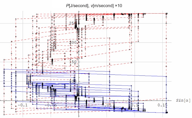
Figure 3 shows locomotive power (P) and speed (v) as functions of the inclination α. The correlation between P and sin(α), and between v and sin(α), is −0.40. A least square fit to linear functions gives P=212+611.7 sin(α) and v=6.18−31.2 sin(α).

Figure 3.

Blue: Locomotive power (P) versus inclination sin(α). Red: Speed (v) ×10 versus inclination sin(α).

Using P(v) for n =4 and b =10 m/second for model 1, we simulated the height and distance as functions of time (t). The agreement between data and simulation was good (Figure 4) since the difference in racing time was 2 seconds for the 815 seconds racing time, with good fit both in uphill and flat terrain. The simulated accumulated distance for the measured time points deviates less than 70 meters from the experimental accumulated distance.

Figure 4.

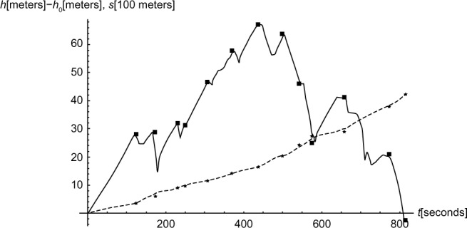
The experimental height (h−h₀) and accumulated distance (s), and simulated height (h−h₀) and accumulated simulated distance (s) as functions of time (t) in seconds.

Notes: h₀ =183 m is initial height. ■ denotes 13 points where time measurements were made for height. The height is relative to initial height in meters; ★denotes 13 points where time measurements were made for accumulated distance. The distance is in units of 100 m; — denotes simulated height (h−h₀); ------ denotes accumulated simulated distance (s).

Figure 5 shows the locomotive power (P) and height (h) as functions of time (t). The skier maintained above 0.90×P_max =248 J/second 62% of the time, with time average of $P_{\text{bas}}^{\mathrm{a}}=232\text{J}/\text{second}$. Figure 6 shows the average experimental and simulated speed, whereas Figure 7 shows the time difference for the 12 track lengths.

Figure 5.

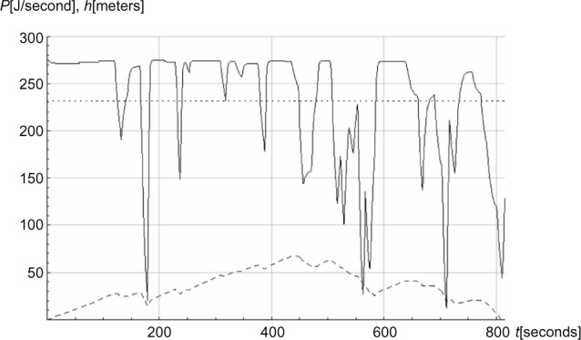
The locomotive power (P) and height (h) of the racing track as functions of time (t) in seconds.

Notes: _____ denotes P(t); -------- denotes average P(t); - - - - - denotes track profile h(t).

Figure 6.

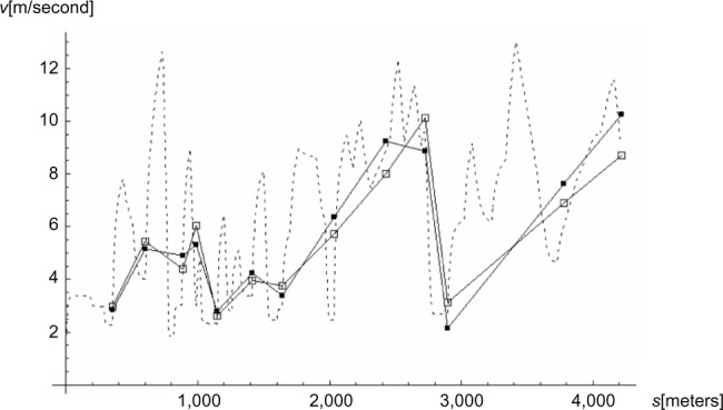
The experimental and simulated average speed, and the simulated speed as functions of accumulated distance (s).

Notes: ■ denotes experimental average speed in m/second; □ denotes simulated average speed in m/second; .... denotes simulated speed in m/second.

Figure 7.

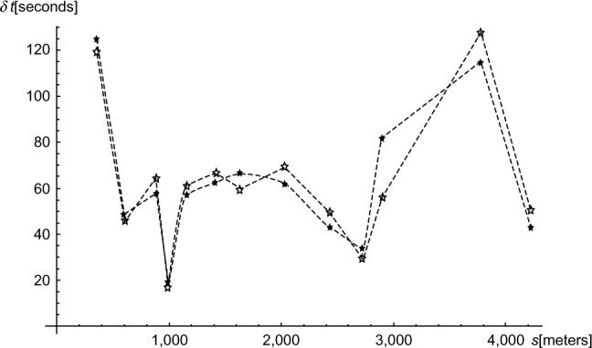
The experimental and simulated time difference (δt) between the points where time measurements were made, as functions of accumulated distance (s).

Notes: ★ denotes experimental time difference between two subsequent points; ✩ denotes simulated time difference between two subsequent points.

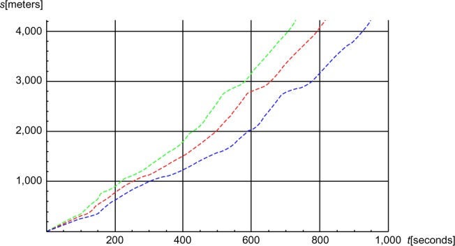
Figures 8–15 show the impact of changes in parameter values relative to the baseline values m=77.5 kg, μ=0.037, ρ=1.29 g/cm³, V=0 m/s, P_max=275 J/second, and the C_dA function as described in detail above. We let χ denote the proportion of mass, friction, density, wind speed, P_max, and C_dA relative to the baseline value of these five symbols and the C_dA function. For example, χ =0.9 means m=69.75 kg, μ=0.0333, ρ=1.161 g/cm³, etc. For wind speed, we let χ denote the wind speed times 0.1. Figure 8 shows the racing time relative to the baseline racing time (hereafter expressed as relative time to complete the race) of 815 seconds as a function of χ; Figure 9 shows the average locomotive power (hereafter expressed as relative locomotive power) P^a relative to the average baseline locomotive power $P_{\text{bas}}^{\mathrm{a}}=232\text{J}/\text{second}$; Figure 10 shows the racing time relative to baseline racing time as a function of $P^{\mathrm{a}}/P_{\text{bas}}^{\mathrm{a}}$; and Figures 11–15 plot the accumulated distance as a function of time for each of the five parameters m, μ, ρ, C_dA, and P_max when the other parameters are held at their baseline values. Finally, to check the sensitivity of the track profile, we included Figure 16, which shows the accumulated distance versus time when using the baseline profile and the profile based on the cubic spline function. Note that this track profile is not more realistic than the chosen piecewise linear track.

Figure 8.

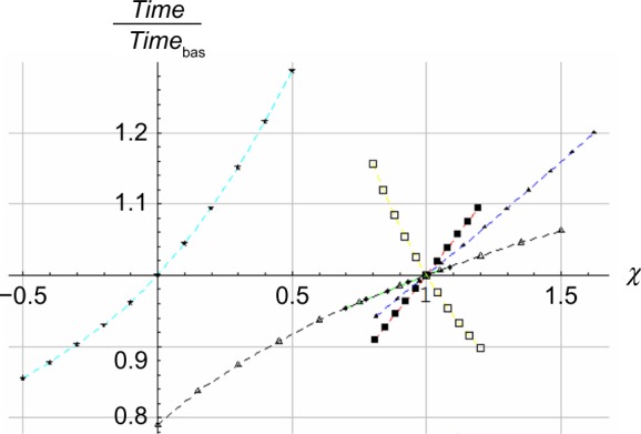
The relative time to complete the race as a function of the proportion χ of the baseline values for m, μ, ρ, V, P_max, and C_dA.

Notes: ■ Red, mass; ▲ blue, friction; ♦ green, density; ★ cyan, wind speed; □ yellow, maximum locomotive power; △ black, drag.

Figure 15.

The accumulated simulated distance (s) in meters as functions of time (t) in seconds.

Notes: Red, baseline; blue, P_max =220 J/second; green, P_max =330 J/second (where P_max is maximum locomotive power).

Figure 9.

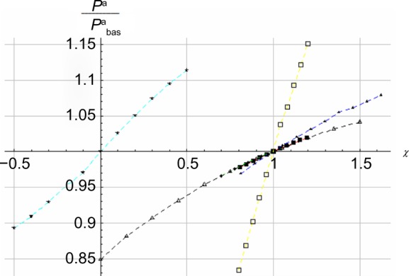
The relative locomotive power $(P^{\text{a}}/P_{\text{bas}}^{\text{a}})$ as a function of the the proportion χ of the baseline values for m, μ, ρ, V, P_max, and C_dA.

Notes: ■ Red, mass; ▲ blue, friction; ♦ green, density; ★ cyan, wind speed; □ yellow, maximum locomotive power; △ black, drag.

Figure 10.

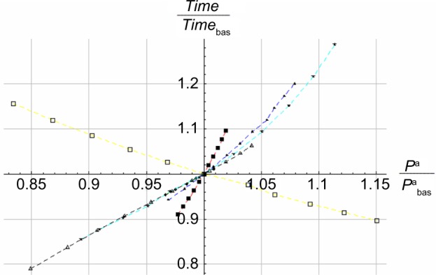
The relative time to complete the race as a function of the relative locomotive power.

Notes: ■ Red, mass; ▲ blue, friction; ♦ green, density; ★ cyan, wind speed; □ yellow, maximum locomotive power; △ black, drag.

Figure 11.

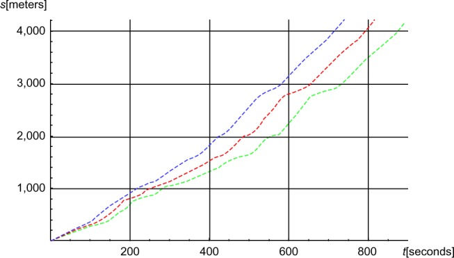
The accumulated simulated distance (s) in meters as functions of time (t) in seconds.

Notes: Red, baseline; blue, m =62.5 kg; green, m =92.5 kg (where m is body mass).

Figure 16.

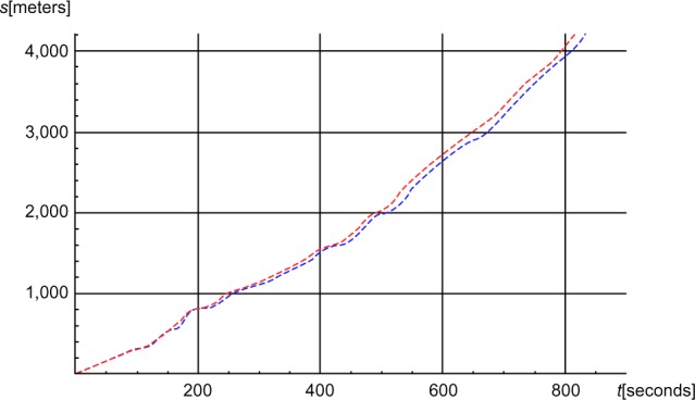
The accumulated simulated distance (s) in meters as functions of time (t) in seconds.

Notes: Red, baseline; blue, cubic spline.

Discussion

In the current study, we adapted the power balance model to simulate cross-country skiing and compared simulated and experimental results for one skier at a self-chosen pace in varying terrain. Here, a model of a skier’s locomotive power as a function of speed was developed, which is a novel modeling approach. The experimental positions of the skier during the race showed a good fit with the simulations, both on uphill and downhill terrain, which support our hypothesis that a skier’s performance in terms of position along the track during a race can be accurately predicted by the power balance model with locomotive power as a function of speed. However, the model needs to be adjusted for each skier, with different locomotive powers and body masses. Furthermore, the locomotive power depends on a variety of physiological parameters such as VO₂max (maximal oxygen consumption), efficiency, technique, and fatigue resistance. We have not yet developed a model that relates locomotive power to these variables, and this remains to be elucidated in future research.

The skier with the highest locomotive power is not necessarily the fastest skier, since different skiers have different friction, drag area, and body mass. Previous studies12,13 contributed to our understanding of the resistant forces caused by ski friction and air drag interacting with locomotive forces. The current simulations extended these previous findings by comparing simulations with experimental data, showing good fit both uphill and downhill. Thus, the power balance model is a useful tool for analyzing cross-country skiing performance on varying terrain. Using this model, we can estimate the influence of changes in various factors such as air drag, friction, and body mass on performance, which is difficult to compare in experimental studies. However, changing these external conditions could even change the technique of a skier and therefore the locomotive power directly. These conditions were maintained constant in our experiment, and we therefore encourage future examinations to address these aspects in more detail.

The logic of the model is such that the two performance measures Time/Time_bas and $P_{\text{bas}}^{\mathrm{a}}$ are approximately linear, especially close to baseline. For example, increasing the skier’s mass 10 kg (from 77.5 to 87.5 kg) increases the runtime from 815 to 868 seconds, ie, 53 seconds, or 6.5%. Furthermore, when decreasing friction from 0.037 to 0.030, the runtime decreases from 815 to 767 seconds, ie, 48 seconds, or 5.9%. The wind speed sensitivity in Figure 8 reveals slight convexity for V>.0 m/second, which is reasonable since increasing headwind makes it increasingly challenging to maintain a high speed. Conversely, increasing tailwind V <0 m/s is initially beneficial, but the benefit decreases, as limits exist for the degree to which tailwind can propel a skier forwards. Air drag in Figure 8 shows slight concavity; that is, a skier with increased projected front area A above the baseline suffers decreasingly as A increases, and benefits increasingly as A decreases below the baseline. Figure 9 reveals sensitivities similar to Figure 7, but $P^{\mathrm{a}}/P_{\text{bas}}^{\mathrm{a}}$ is almost linear for wind speed.

Figure 2 shows that increasing locomotive power (P) corresponds to decreasing skier speed (v). The reason, explained in Equation 3, is the dependence of v on α, which means that in steep uphill terrain, with high α, speed (v) is low and locomotive power (P) is high. This is illustrated more thoroughly in Figure 3, which shows how P increases with α, and how v decreases with α.

Figure 10 shows some linearity close to the baseline, and slight convexity as $P^{\mathrm{a}}/P_{\text{bas}}^{\mathrm{a}}$ increases above the baseline, especially for wind speed (V). That is, exerting average locomotive power above the baseline causes increasing time to complete the race due to increased mass, friction, density, wind speed, and drag, but not due to increased maximum locomotive power (yellow curve with unfilled boxes), which causes increased $P^{\mathrm{a}}/P_{\text{bas}}^{\mathrm{a}}$ and thereby decreased Time/Time_bas. Hence, the curves in Figure 10 proceed through the first and third quadrants, except for the curve for maximum locomotive power, which proceeds through the second and fourth quadrants. Since the estimated effects of the abovementioned changes in various factors on performance are difficult to investigate with experimental methods, using such simulation models provides complementary understanding.

Along the same line, Figures 11–15 enable us to assess how the accumulated distance s varies as a function of time to complete the race when five parameters are altered with fixed amounts below and above their baseline values. Sensitivity analysis of the kind illustrated in Figures 8–15 provide a rich tool, illustrating how models like the one presented in this paper can be applied in practice, answering specific questions about how performance measures such as time to complete the race and locomotive power are impacted by changes in parameter values. Finally, Figure 16 shows the difference between the accumulated distance versus time when using the baseline profile and the profile based on the cubic spline function.

More generally, researchers, coaches, and ski preparers can use the model in this paper to estimate how performance is impacted by changes in the parameters. To extend upon our model, future research can conduct more extensive sensitivity analysis for these parameters, plot the performance measures in three dimensions as functions of the parameters to illustrate nonlinearities, conduct sensitivity analysis for various track profiles expressed with the inclination α changing differently as a function of time, and can conduct sensitivity analysis for performance dependent on changes in technique.

As an alternative to letting the exogenously given locomotive power P in Equation 3 and Figure 2 be a function of speed, future research can endogenize P into the model or let P vary as a function of speed and, in addition, incline, mass, friction, density, wind speed, maximum locomotive power, and projected front area, where additionally speed depends on these other parameters. Some speculation has been made as to whether locomotive power P is better simulated as a function of the terrain’s incline α. Here, the hypothesis is that on steep climbs, the skier generates maximum locomotive power. As incline decreases to near flat, locomotive power smoothly decreases from the maximum. On downhill inclines, locomotive power decreases toward zero as the incline steepens. However, experience shows that the skier when moving downhill accelerates to a certain speed before choosing the deep-tuck posture for speeds above approximately 10 m/second for any decline. Similarly, when transitioning from flat to uphill, it takes some time until locomotive power P has stabilized as a function of incline. We thus propose that if the P(α) dependence of locomotive power on incline α is researched, this dependence is considered under stationary conditions, with additional theory building for the transitions in incline. More generally, the locomotive power P can be endogenized more thoroughly into the model equations (Equations 1 and 2).

To further improve the simulation model, the track profile has to be much more accurately monitored. Additionally, more data on how locomotive power and efficiency change across the different skating techniques, speeds, and inclines in the terrain would be advantageous. For example, we find the greatest differences between the simulation and the experimental data on terrain with rapidly changing curvature. Another interesting objective is to establish a more detailed and generic model on how the skier changes the intensity on uphill and downhill terrain.

Figure 12.

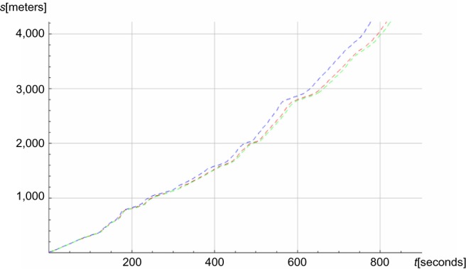
The accumulated simulated distance (s) in meters as functions of time (t) in seconds.

Notes: Red, baseline; blue, ρ =0.90 g/cm³; green, ρ =1.40 g/cm³ (where ρ is air density).

Figure 13.

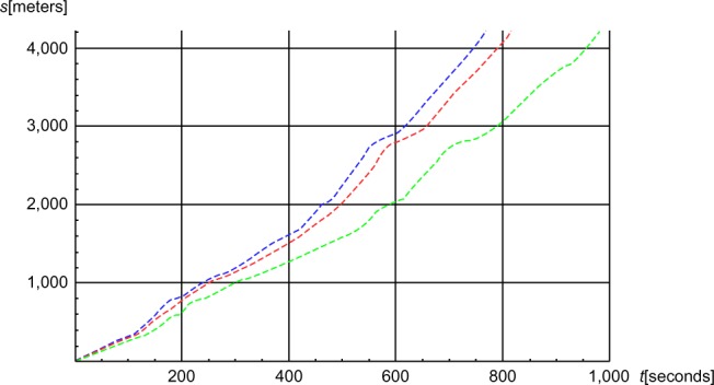
The accumulated simulated distance (s) in meters as functions of time (t) in seconds.

Notes: Red, baseline; blue, μ =0.03; green, μ =0.06 (where μ is the friction coefficient).

Figure 14.

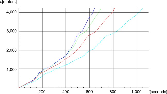
The accumulated simulated distance (s) in meters as functions of time (t) in seconds.

Notes: Red, baseline; blue, C_dA =0; green, −5 m/second tailwind; cyan, +5 m/second headwind (where C_d is the drag coefficient, and A is the projected front area of the skier).

References

- 1.Bergh U, Forsberg A. Influence of body mass on cross-country ski racing performance. Med Sci Sports Exerc. 1992;24(9):1033–1039. [PubMed] [Google Scholar]
- 2.Norman RW, Komi PV. Mechanical energetics of world-class cross-country skiing. Int J Sport Biomech. 1987;3:353–369. [Google Scholar]
- 3.Smith GA. Biomechanical analysis of cross-country skiing techniques. Med Sci Sports Exerc. 1992;24(9):1015–1022. [PubMed] [Google Scholar]
- 4.Sandbakk O, Ettema G, Holmberg HC. The influence of incline and speed on work rate, gross efficiency and kinematics of roller ski skating. Eur J Appl Physiol. 2012;112(8):2829–2838. doi: 10.1007/s00421-011-2261-0. [DOI] [PubMed] [Google Scholar]
- 5.Moxnes JF, Sandbakk Ø, Hausken K. A simulation of cross-country skiing on varying terrain by using a mathematical power balance model. Open Access J Sports Med. 2013;4:127–139. doi: 10.2147/OAJSM.S39843. [DOI] [PMC free article] [PubMed] [Google Scholar]
- 6.Sandbakk O, Ettema G, Leirdal S, Jakobsen V, Holmberg HC. Analysis of a sprint ski race and associated laboratory determinants of world-class performance. Eur J Appl Physiol. 2011;111(6):947–957. doi: 10.1007/s00421-010-1719-9. [DOI] [PMC free article] [PubMed] [Google Scholar]
- 7.Sandbakk O, Holmberg HC, Leirdal S, Ettema G. Metabolic rate and gross efficiency at high work rates in world class and national level sprint skiers. Eur J Appl Physiol. 2010;109(3):473–481. doi: 10.1007/s00421-010-1372-3. [DOI] [PubMed] [Google Scholar]
- 8.de Koning JJ, Bobbert MF, Foster C. Determination of optimal pacing strategy in track cycling with an energy flow model. J Sci Med Sport. 1999;2(3):266–277. doi: 10.1016/s1440-2440(99)80178-9. [DOI] [PubMed] [Google Scholar]
- 9.de Koning JJ, van Ingen Schenau GJ. On the estimation of mechanical power in endurance sports. Sports Sci Rev. 1994;3:34–54. [Google Scholar]
- 10.van Ingen Schenau GJ, Jacobs R, de Koning JJ. Can cycle power predict sprint running performance? Eur J Appl Physiol Occup Physiol. 1991;63(3–4):255–260. doi: 10.1007/BF00233857. [DOI] [PubMed] [Google Scholar]
- 11.Moxnes JF, Hausken K. Cross-country skiing motion equations, locomotive forces and mass scaling laws. Math Comp Model Dynamic Syst. 2008;14(6):535–569. [Google Scholar]
- 12.Sundstrøm D, Carlsson P, Ståhl F, Tinnsten M. Numerical optimization of pacing strategy in cross-country skiing. Struct Mulitidisc Optim. 2013;47:943–950. [Google Scholar]
- 13.Carlsson P, Tinnsten M, Ainegren M. Numerical simulation of cross-country skiing. Comput Methods Biomech Biomed Engin. 2011;14(8):741–746. doi: 10.1080/10255842.2010.493885. [DOI] [PubMed] [Google Scholar]
- 14.van Ingen Schenau GJ, Cavanagh PR. Power equations in endurance sports. J Biomech. 1990;23(9):865–881. doi: 10.1016/0021-9290(90)90352-4. [DOI] [PubMed] [Google Scholar]
- 15.Leirdal S, Saetran L, Roeleveld K, et al. Effects of body position on slide boarding performance by cross-country skiers. Med Sci Sports Exerc. 2006;38(8):1462–1469. doi: 10.1249/01.mss.0000227536.13175.52. [DOI] [PubMed] [Google Scholar]
- 16.Spring E, Savolainen S, Erkkila J, Hamalainen T, Pihkala P. Drag area of cross-country skier. Int J Sport Biomech. 1988;4:103–113. [Google Scholar]
- 17.Andersson E, Supej M, Sandbakk O, Sperlich B, Stoggl T, Holmberg HC. Analysis of sprint cross-country skiing using a differential global navigation satellite system. Eur J Appl Physiol. 2010;110(3):585–595. doi: 10.1007/s00421-010-1535-2. [DOI] [PubMed] [Google Scholar]