Balanced Cortical Microcircuitry for Spatial Working Memory Based on Corrective Feedback Control

Abstract

A hallmark of working memory is the ability to maintain graded representations of both the spatial location and amplitude of a memorized stimulus. Previous work has identified a neural correlate of spatial working memory in the persistent maintenance of spatially specific patterns of neural activity. How such activity is maintained by neocortical circuits remains unknown. Traditional models of working memory maintain analog representations of either the spatial location or the amplitude of a stimulus, but not both. Furthermore, although most previous models require local excitation and lateral inhibition to maintain spatially localized persistent activity stably, the substrate for lateral inhibitory feedback pathways is unclear. Here, we suggest an alternative model for spatial working memory that is capable of maintaining analog representations of both the spatial location and amplitude of a stimulus, and that does not rely on long-range feedback inhibition. The model consists of a functionally columnar network of recurrently connected excitatory and inhibitory neural populations. When excitation and inhibition are balanced in strength but offset in time, drifts in activity trigger spatially specific negative feedback that corrects memory decay. The resulting networks can temporally integrate inputs at any spatial location, are robust against many commonly considered perturbations in network parameters, and, when implemented in a spiking model, generate irregular neural firing characteristic of that observed experimentally during persistent activity. This work suggests balanced excitatory–inhibitory memory circuits implementing corrective negative feedback as a substrate for spatial working memory.

Introduction

Working memory refers to an ability to hold information “on-line” in the absence of sensory inputs. In spatial working memory, the item held in memory is the spatial location of an object that must be recalled after a delay period of up to several seconds. Electrophysiological recordings have revealed neurons in the parietal and frontal cortices that encode the remembered location of a cue through spatially tuned patterns of persistent neural firing (Funahashi et al., 1989; Constantinidis and Steinmetz, 1996; Chafee and Goldman-Rakic, 1998), but the circuit mechanisms maintaining this sustained neural activity remain poorly understood.

Computational modeling has been useful in suggesting possible mechanisms for the generation and storage of spatially specific patterns of persistent neural activity. The vast majority of models consist of networks of excitatory and inhibitory neuronal populations connected by short-range excitation and longer range inhibition (for review, see Ermentrout, 1998; Compte, 2006). Local recurrent excitation between neurons having similar preferred features provides positive feedback that supports long-lasting reverberation of activity, while long-range inhibition stabilizes and shapes the spatially localized patterns of activity. However, although long-range inhibition could be achieved through disynaptic pathways (Melchitzky et al., 2001) or large basket cells (Markram et al., 2004), the neural substrate for widespread inhibition in memory circuits remains unclear because inhibitory projections are typically shorter ranged than excitatory projections (Braitenberg and Schüz, 1998; Douglas and Martin, 2004).

Recent studies of frontal cortical microcircuitry suggest an alternative mechanism, based on negative-derivative feedback rather than positive feedback, may play a critical part in maintaining persistent neural activity. The key experimental observations motivating this hypothesis are that, first, inhibitory and excitatory inputs have been suggested to be balanced in strength in frontal cortical neurons (Shu et al., 2003; Haider et al., 2006) or more generally positively covary in other cortical neurons (Rudolph et al., 2007; Haider and McCormick, 2009), and, second, the kinetics of excitatory-to-excitatory synaptic connections are slower than those of excitatory-to-inhibitory connections (Wang et al., 2008; Wang and Gao, 2009; Rotaru et al., 2011). Recent modeling work (Lim and Goldman, 2013) has shown how these two conditions provide a mechanism for maintaining persistent activity through negative-derivative feedback that opposes drifts in firing rate: changes in firing rate trigger fast negative feedback that opposes the drift, followed by slower excitatory feedback that rebalances the net synaptic input. Here, we show how such negative-derivative feedback can operate in a spatially specific manner to maintain spatial working memory. Unlike traditional spatial working memory networks that have stereotyped spatial profiles of activity, and thus lose information about stimulus amplitude, we show that negative-derivative feedback models can temporally integrate their inputs and store analog values of stimulus amplitudes as well as spatial locations. Furthermore, by examining the relationship between the structure of the synaptic connectivity and the spatial profiles of persistent activity, we show that derivative-feedback memory networks do not require widespread, lateral inhibition. Finally, we show that the balance of inhibition and excitation that underlies persistent activity is robustly maintained across a range of common perturbations and leads to irregular neuronal firing similar to that observed experimentally (Compte et al., 2003).

Materials and Methods

Here we describe how our firing rate and spiking networks are structured to maintain spatially tuned patterns of persistent firing through a negative-derivative feedback mechanism. Consistent with experimental observations in prefrontal cortex (Goldman-Rakic, 1995), the model networks are organized in a functionally columnar architecture of excitatory and inhibitory neurons (Fig. 1) with each column defined by having a similar preferred spatial feature of the stimulus. Following previous work (Ermentrout, 1998; Wang, 2001; Compte, 2006), we assume that these preferred spatial features are uniformly distributed along a ring and can be characterized by an angular variable θ. Below, we first describe the network structure and equations governing the dynamics of both the firing rate and spiking models. Then, we analytically derive conditions for producing spatially localized persistent activity in networks with either linear or nonlinear dynamics, and with or without translation-invariant symmetry.

Figure 1.

Structure of network model for spatial working memory. We consider a columnar architecture of excitatory and inhibitory neurons such that neurons in the same column have similar preferred feature θ. The connectivity strength J is dependent only on the preferred features θ and θ′ of the presynaptic and postsynaptic neurons and τ represents the decay time of synaptic currents at the shown connections. Blue and red curves represent excitatory and inhibitory connections, respectively.

Firing rate model of spatial memory network.

In the firing rate models, the activities of, and synaptic interactions between, the neurons are parameterized by their preferred spatial feature θ, which ranges from –π to π. The dynamics of the firing rates and synaptic state variables are governed by the equations:

where r_i(θ,t) represents the mean firing rate of the excitatory (E) or inhibitory (I) population i with preferred feature θ. s_ij(θ′,t) denotes the synaptic state variable for the connections from population j with preferred feature θ′ onto population i for i,j = E or I, and approaches the presynaptic firing rate r_j(θ′,t) with time constant τ_ij.

The mean firing rate r_i(θ,t) approaches f_i(x_i(θ,t)) with intrinsic time constant τ_i, where f_i(x) represents the steady-state neuronal response to input current x. We consider two types of neuronal response functions: linear f(x) = x (Figs. 4, 5A–D, top, 6–10) and a nonlinear neuronal response function (Fig. 5A–D, bottom) having the Naka–Rushton (Wilson, 1999) form

where M represents the maximal neuronal response, x_θ represents the input threshold, x₀ defines the value of (x − x_θ) at which f(x) reaches its half-maximal value, and h(x) denotes the step function h(x) = 1 for x ≥ 0 and h(x) = 0 for x < 0.

Figure 4.

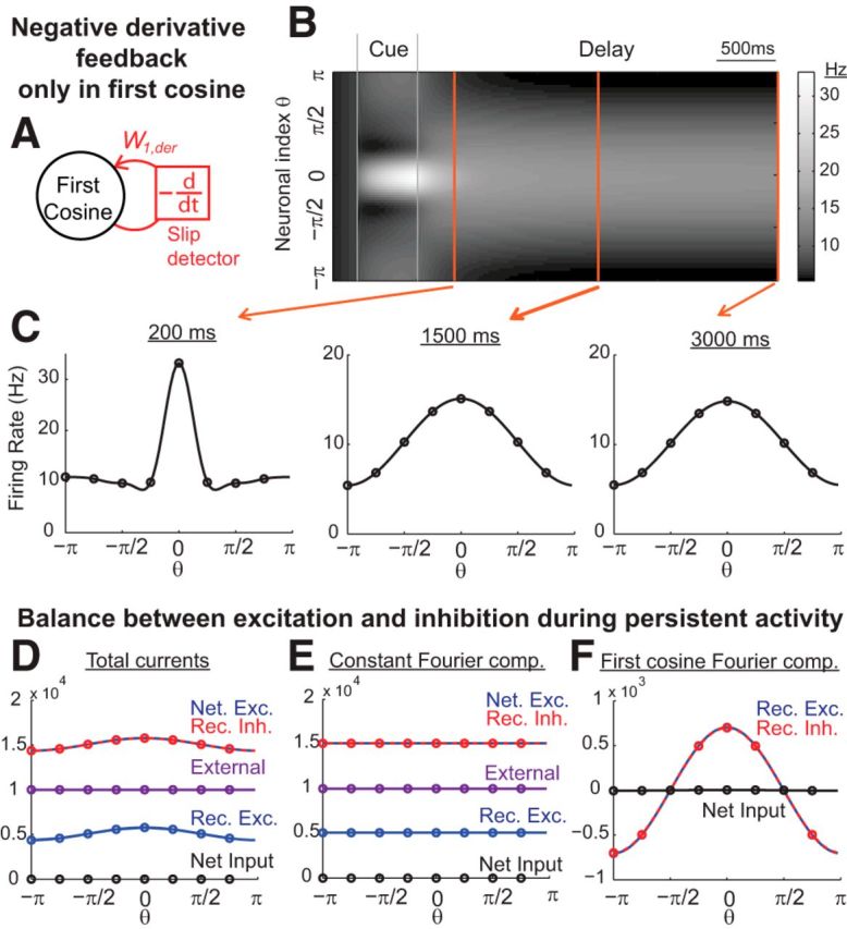
Temporal evolution of activity and balance between excitation and inhibition during memory performance. A, Example network with negative-derivative feedback only in the first cosine component. B, Grayscale-coded spatiotemporal activity pattern. The x-axis represents time and the y-axis represents the neuronal index parameterized by its preferred cue direction θ. C, Spatial profiles of firing activity at different times corresponding to the orange vertical slices in B. D–F, Close balance between excitation and inhibition during the delay period. The shown neuron receives strong net excitation and inhibition that are balanced in strength. The first cosine Fourier component, but not the constant Fourier component, is maintained by negative-derivative feedback, as indicated in F by the balance of recurrent excitation with recurrent inhibition within this first cosine component. Values in D–F are illustrated for the inputs onto an excitatory neuron at 3 s into the delay period.

Figure 5.

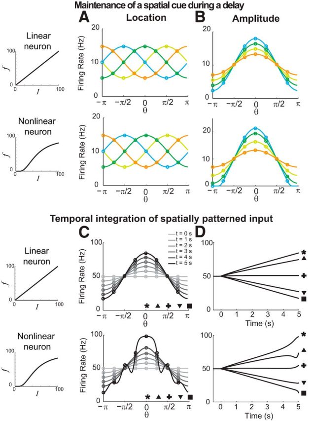
Location codes, amplitude codes, and temporal integration of negative-derivative feedback networks with linear (top) and nonlinear (bottom) firing rate (f) versus input current (I) relationships. A, Maintenance during the delay period of spatial patterns of activity centered at different locations in the network, corresponding to different spatial cues (shown as different colors). B, Maintenance of spatial patterns of activity of different amplitudes during a delay period for inputs at the same spatial location but with different strengths. Input amplitudes for the linear case were smaller than those for the nonlinear case to avoid the negative firing rates that are permitted in linear networks. C, D, Temporal integration of spatially structured input. After time 0, a spatially structured input is continuously present and the amplitude of the spatial pattern of activity linearly increases in time (C), resulting in ramp-like changes (D). Patterns in A and B are shown at 3 s into the delay period. In C and D (bottom), the ripply activity pattern at t = 5 s reflects the effect of reaching the extreme, saturating limit of the neuronal response function, when the neuron with preferred location θ = 0 has approached its limiting firing rate of 100 Hz and becomes insensitive to additional input.

Figure 6.

Networks receiving negative-derivative feedback in multiple Fourier components and maintenance of multiple bumps of activity. A, B, Example networks with negative-derivative feedback in multiple Fourier components (A). The synaptic connectivity profiles for this example were Gaussian shaped (B). C, D, The presence of negative-derivative feedback in higher order Fourier components permits the maintenance of narrowly tuned patterns of activity (C) and multiple bumps of activity (D). Data in C and D are shown at 3 s into the delay period.

Figure 7.

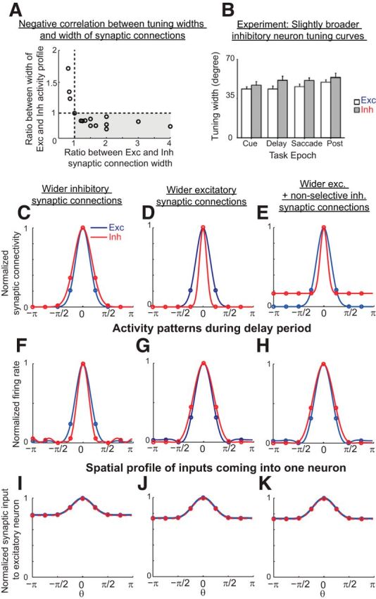
Maintenance of spatially localized, persistent activity with short-range inhibition and long-range excitation and relation between the profile of synaptic connectivity and the tuning widths of activity. A, Negative correlation between tuning widths and width of synaptic connections in negative-derivative feedback networks. The spatial profiles of the excitatory and inhibitory connections in this example were Gaussian, and the widths of both the excitatory and inhibitory connections were varied. To obtain the tuning widths of the activity of the excitatory and inhibitory populations, the activity was fit by the sum of constant and Gaussian functions and the tuning width was defined as the width of the Gaussian function during the delay period as in Constantinidis and Goldman-Rakic, (2002). B, Experimentally observed broader tuning of inhibitory neurons than of excitatory neurons during the different task epochs of a delayed saccade task. (Adapted from Constantinidis and Goldman-Rakic, 2002). C–E, Spatial profile of excitatory (blue; same for the E-to-E and E-to-I connections) and inhibitory (red; same for the I-to-E and I-to-I connections) connectivity with broader inhibitory connections (C), broader excitatory connections (D), or broader tuned component of excitatory than inhibitory connections but with inhibitory connections additionally having a nonselective (constant) component (E). Spatial profiles of synaptic connectivity are normalized by their maximum height. F–H, Activity patterns of excitatory (blue) and inhibitory (red) populations in response to a stimulus centered at θ = 0, illustrated 3 s into the delay period. Firing rates were normalized for comparison by subtracting off the minimum activity and scaling the resulting firing rates to unit amplitude. A broader tuned component of the inhibitory connections (C) results in a narrower profile of the inhibitory population activity (F). A broader tuned component of excitatory connections, with (E) or without (D) an additional nonselective component of inhibitory projections, results in a narrower profile of sustained excitatory activity (G, H). I–K, Spatial profiles of balanced excitatory (blue) and inhibitory (red) synaptic inputs coming into an excitatory neuron. Inputs are normalized by the maximum of the excitatory inputs.

Figure 8.

Comparison of activity patterns and synaptic inputs with spatial memory networks without negative-derivative feedback networks that have equal timescales for positive and negative feedback pathways. A–H, Network structures and spatial profile of synaptic connectivity. For simplicity, the E-to-E (blue), E-to-I (green), and I-to-E (red) connections without the I-to-I connection are included and the spatial profile of synaptic connectivity is normalized by its maximum height (E–H). I–L, Activity patterns of excitatory (blue) and inhibitory (red) populations in response to a stimulus centered at θ = 0 (3 s into the delay period). When both the E-to-I and I-to-E connections are narrow, the network cannot sustain spatially localized activity, resulting in spatially uniform activity. Firing rates were normalized for comparison by subtracting off the minimum activity and scaling the resulting firing rates to unit amplitude except for the case showing spatially uniform patterns of activity (I). With broader negative feedback (B–D, F–H), spatially localized activity can be stabilized, with broader tuning of the inhibitory population. M–P, Spatial profiles of balanced excitatory (blue) and inhibitory (red) synaptic inputs coming into an excitatory neuron. Inputs are normalized by the maximum of the excitatory inputs. The networks receive broader inhibitory than excitatory inputs for spatially localized activity, resulting in an overall Mexican-hat (i.e., center-surround) type input (N–P).

Figure 9.

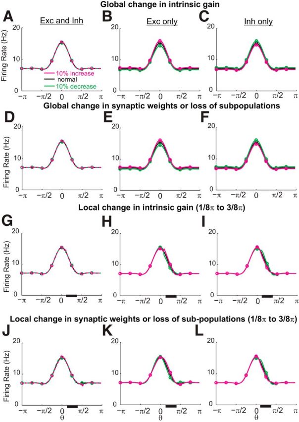
Robustness to common perturbations in memory networks with negative-derivative feedback. The networks can maintain spatially localized, persistent activity robustly against either global (A–F) or local (G–L) perturbations that preserve the balance between excitation and inhibition such as changes in intrinsic gain (A–C, G–I) or changes in synaptic weights or loss of a fraction of the neurons in a given subpopulation (D–F, J–L). The local perturbations were in neurons whose preferred directions lie between 1/8π and 3/8 π, represented by the black bar along the x-axis. Activity profiles are shown for 3 s into the delay period.

Figure 10.

Memory performance following perturbations under which the E-I balance is maintained (A–D) or disrupted (E–H). A–D, Time course of activity under global (A, B) or local (C, D) perturbations in all excitatory synaptic weights, or equivalently under loss of a corresponding fraction of the excitatory subpopulation. Since loss of a fraction of the cells or of all excitatory synapses affects both the positive and negative feedback pathways equally, the balance between positive and negative feedback is maintained and persistent firing is minimally affected. The time course of activity is shown for an example neuron receiving an external input stimulus centered on its preferred direction and for an example neuron receiving external input in its nonpreferred directions. E–H, Disruption of persistent firing under global (E, F) or local (G, H) perturbations in the E-to-E connections, mimicking perturbations in slow NR2B subunit-containing NMDA receptors located predominantly in this connection (Wang et al., 2013). Global perturbations led to similar changes in activity throughout the entire network (E, F), while local perturbations disrupted activity most severely in the perturbed neurons (G, H). I, J, Time constant of activity decay τ_eff in a neuron receiving an external input stimulus centered on its preferred direction as a function of the strengths of positive and negative feedback pathways. τ_eff is estimated by fitting the time course of delay activity between 500 and 2000 ms with an exponential function. As the overall strengths J_pos and J_neg of the positive and negative feedback pathways change, τ_eff decays approximately in inverse proportion to 1 − J_pos/J_neg (linear change in 1/|τ_eff| in I). Local perturbations (data not shown) provided similar results. In J, J_neg was fixed and only J_pos changed, corresponding to the red arrow in I. The black fit curve is given by 0.075 sec/|1 − J_pos/J_neg|∼(τ_pos − τ_neg)/(1 − J_pos/J_neg).

The input x_i(θ,t) to population i with the preferred feature θ is a sum of the recurrent synaptic currents J_ij(θ,θ′) s_ij(θ′,t) from population j with the preferred feature θ′ and the external current i_i(θ,t) (not to be confused with the subscript i). J_ij(θ,θ′) represents the synaptic connectivity strength and, except for the nontranslationally invariant model described in the final section of the Materials and Methods, we assume that it depends only on the distance between θ and θ′ and can be rewritten as J_ij(θ − θ′). In Figures 6–10, we consider networks with Gaussian-shaped profiles of synaptic connectivity J_ij(θ − θ′) = J_ij exp[ − (θ − θ′)²/σ_ij²], where σ_ij here and below denotes $\sqrt{2}$ times the standard deviation of the Gaussian. In Figures 4 and 5, in which only the first cosine Fourier component is tuned to provide negative-derivative feedback, we consider networks that have a (different) Gaussian-shaped profile, plus additional constant and cosine components J_ij(θ − θ′) = J_ij,const + J_ij,cos cos(θ − θ′) + J_ij,gaus exp[ − (θ − θ′)²/σ_ij²].

We assume that the external input i_i(θ,t) is the sum of constant background input i_i,c and time-varying input, where the time-varying component can be expressed separably as the product of a spatial component i_i,s(θ) and a temporal component i_i,t(t), so that i_i(θ,t) = i_i,c + i_i,s(θ) i_i,t(t). The temporal component i_i,t(t) represents an external pulse of input that has undergone smoothing before its arrival at the memory network, and is modeled as a pulse of duration t_window = 500 ms that is exponentially filtered with time constant τ_ext = 100 ms. The spatial component i_i,s(θ) is a Gaussian function centered at θ₀. For the unimodal activity described in most of the paper, i_i,s(θ) = i_i,s,0 + i_i,s,1 exp[ − (θ − θ₀)²/σ_iO²]. For the multi-modal activity in Figure 6D, it is the sum of Gaussian functions i_i,s(θ) = i_i,s,0 + ∑_k=1³ i_i,s,1^k exp[ − (θ − θ₀^k)²/(σ_iO^k)²], where the superscript k denotes the Gaussian component and is not an exponent. For the temporal integration of spatially localized input in Figure 5, i_i,s(θ) is given by i_i,s(θ) = i_i,s,0 + i_i,s,1 cos(θ − θ₀).

Throughout the paper except in Figure 8, the intrinsic time constants of excitatory and inhibitory neurons, τ_E and τ_I, are 20 and 10 ms, respectively (McCormick et al., 1985). The time constants of GABA_A-type inhibitory synapses, τ_EI and τ_II, are each 10 ms (Salin and Prince, 1996; Xiang et al., 1998). Based upon experimental measurements of excitatory synaptic currents in prefrontal cortex (Rotaru et al., 2011), the time constants of excitatory synaptic currents, τ_EE and τ_IE, were set to 100 and 25 ms, respectively. Note that these time constants reflect the kinetics of postsynaptic potentials triggered by activation of NMDA- and AMPA-type receptors, but likely include the effects of additional intrinsic ionic conductances since these experiments were performed without blocking intrinsic ionic currents (Rotaru et al., 2011).

For the nonlinear function of Naka–Rushton form in Equation 2, the maximal response M = 100, the half-activation parameter x₀ = 40, and the input threshold x_θ = 10. The parameters for the spatial components of the synaptic connectivity and external input were assigned as follows: in Figures 4 and 5, the parameters for the Gaussian component of the connectivity are J_EE,gaus = 50/π, J_IE,gaus = J_EI,gaus = J_II,gaus = 100/π, σ_EE= σ_IE = σ_EI = σ_II = 0.2π. The parameters for the amplitudes of the constant and cosine terms of the connectivity were defined as J_EE,const = 250/π − J_EE,gaus a₀, J_IE,const = J_EI,const = J_II,const = 300/π − J_IE,gaus a₀, J_EE,cos = 150/π − J_EE,gaus a₁, J_IE,cos = 300/π − J_IE,gaus a₁, J_EI,cos = 100/π − J_EI,gaus a₁, J_II,cos = 200/π − J_II,gaus a₁, where a₀ and a₁ are multiplicative factors deriving from the constant and first cosine components of the Gaussian portion of the connectivity, and are defined as $a_0=\frac{1}{2\pi }{\displaystyle {\int }_{-\pi }^{\pi }d\theta \exp \left[-{\left(\theta /0.2\pi \right)}^2\right]\approx 0.1\sqrt{\pi }}$ and $a_1=\frac{1}{\pi }{\displaystyle {\int }_{-\pi }^{\pi }d\theta \cos (\theta )\exp \left[-{\left(\theta /0.2\pi \right)}^2\right]\approx 0.2e^{-0.01{\pi }^2}\sqrt{\pi }}$. With these definitions, the overall first cosine component of the connectivity satisfied the balance condition of Equation 9 below. σ_EO = 0.25π, i_Ec = 10,000, i_Ic = 9000, i_E0 = 500, i_I0 = 0, and i_I1 = 0 in Figures 4 and 5A,B. i_E1 = 300 in Figures 4 and 5A, varies between 200 and 500 in Figure 5B, top, and varies between 200 and 800 in Figure 5B, bottom. i_Ec = 5000, i_Ic = 0, i_I0 = i_I1 = 0, i_E0 = i_E1 = 80 in Figure 5C,D. The parameters in Figures 6–9 are the following: J_EE,1 = 100, J_IE,1 = 200, J_EI,1 = 100, J_II,1 = 200, σ_EE = σ_IE = 0.1π, σ_EI = σ_II = 0.2π, σ_EO = 0.4π, i_Ec = i_Ic = 0, i_E0 = 100, i_I0 = 0, i_E1 = 135, and i_I1 = 0, except in Figure 6D where i_E0 = 100, i_I0 = 0, i_I1 = 0, and i_E,1¹ = 150, i_E,1² = i_E,1³ = 100, θ₀¹ = 0, θ₀^2,3 = ± 2π/3 and σ_EO^1,2,3 = π/6.

In the spatial working memory networks without negative-derivative feedback (Fig. 8), τ_EE and τ_IE equal 100 ms, and the remaining time constants are the same as the corresponding ones for the negative-derivative feedback networks. The neuronal response (input current–output firing rate) functions in this figure were chosen to be linear for the inhibitory neurons and, for the excitatory neurons, a piecewise linear function given by f(x) = 1.4(x − 1) + 3.5 for x < 1, f(x) = 14(x − 1) + 3.5 for 1 ≤ x < 2, and f(x) = 7(x − 2) + 17.5 for 2 ≤ x. The spatial component of the synaptic connectivity is a Gaussian function J_ij(θ − θ′) = J_ij exp[ − (θ − θ′)²/σ_ij²] with no I-to-I connection (and, for Fig. 8D,H,L,P only, with the addition of a constant function). The corresponding parameters are as follows: J_EE,gaus= J_IE,gaus = 0.5/π, J_EI,gaus = 2.5/π, σ_EE = σ_IE = 0.2π, σ_EI = 0.1π for Figure 8A, E, I, and M; J_EE,gaus = 0.5/π, J_IE,gaus = 1/π, J_EI,gaus = 0.5/π, σ_EE = 0.2π, σ_IE = π, σ_EI = 0.1π for Figure 8B, F, J, and N; J_EE,gaus= J_IE,gaus = J_EI,gaus = 0.5/π, σ_EE= σ_IE = 0.2 π, σ_EI = π for Figure 8C, G, K, and O; and J_EE,gaus= J_EI,gaus = 0.5/π, J_IE,gaus = 1/π, σ_EE= σ_IE = 0.2π, σ_EI = 0.1π, and with the addition of a constant value 0.1/π to the I-to-E connection for Figure 8D,H, L, and P. The spatial profile of the transient external input is the same for all networks and is given by i_i,s(θ) = 0.5 + 0.5 cos(θ).

All the simulations of the firing rate models were run with a fourth-order explicit Runge–Kutta method in MATLAB.

Spiking network of leaky integrate-and-fire neurons.

In Figure 11, we constructed a recurrent network of excitatory and inhibitory populations of spiking neurons with balanced excitation and inhibition. The activities of, and synaptic interactions between, the neurons are parameterized by their preferred spatial feature θ, which ranges from –π to π, as in the firing rate models. Here, we describe the intrinsic dynamics of the individual neurons and the synaptic currents connecting the neurons.

Figure 11.

Irregular firing in spiking networks. A, Experimentally measured irregular firing, as captured by the local coefficient of variation CV₂ during persistent activity in a delayed-saccade tasks. (Adapted from Compte et al., 2003). B–H, Simulation of spiking network models with negative-derivative feedback. B, Activity of excitatory neurons during the delay period in response to a transient, Gaussian-shaped stimulus. The firing rate distribution shown represents averages of neuronal activity between 2500 and 3000 ms after the stimulus offset (black curve) and is fit with a sum of constant and Gaussian functions (gray curve). C–H, Activity of neurons receiving a stimulus in their preferred directions (C–E, computed for neurons 7601–8400 in B) or neurons receiving stimuli in their nonpreferred directions (F–H, computed for neurons 1–400 and 15601–16000). C, F, Instantaneous, population-averaged activity, computed within time bins of 1 ms (gray) or 10 ms (black). Vertical red lines indicate the times of the start and end of the stimulus. D, G, Raster plots illustrating the irregular persistent firing of 40 example neurons. E, H, Histogram of CV₂ values of active neurons during the persistent firing. Note that, for the activity of neurons receiving preferred stimuli, a small set of neurons fired regularly at high firing rate and exhibited low CV₂ values. This is due to the heterogeneity of our completely randomly connected networks, resulting in excess positive feedback in some clusters of neurons.

The spiking network consists of N_E excitatory and N_I inhibitory current-based leaky integrate-and-fire neurons that emit a spike when a threshold is reached and then return to a reset potential after a brief refractory period. The neurons are recurrently connected to each other and receive transient stimuli from an external population of N_O neurons. The connectivity between neurons is sparse and random with constant connection probability ρ_i so that, on average, each neuron receives N_Eρ_E, N_Iρ_I, and N_Oρ_O synaptic inputs from the excitatory, inhibitory, and external populations, respectively. The strengths of the recurrent connections and connections from the external population are dependent on the difference between the preferred feature θ of the postsynaptic neuron and the preferred feature θ′ of the presynaptic neuron.

The dynamics of the subthreshold membrane potential V_i^l of the lth neuron in population i and the dynamics of the synaptic input variables s_ij^lm onto this neuron from the mth neuron in population j are given as follows:

The first term on the right-hand side of Equation 3 corresponds to a neuronal intrinsic leak process such that, without the input, the voltage decays to the resting potential V_L with time constant τ_i. The second term is the sum of the recurrent NMDA- and AMPA-mediated excitatory synaptic currents. The dynamic variables s_iE^lm,N and s_iE^lm,A represent NMDA- and AMPA-mediated synaptic currents from cell m of the excitatory population. The fractions of NMDA- and AMPA-mediated currents are assumed to be uniform across the population and are denoted by q_iE^N and q_iE^A = 1 − q_iE^N, respectively. p_iE^lm is a binary random variable with probability ρ_E and represents the random connectivity between neurons. The sum of the strengths of the NMDA- and AMPA-mediated synaptic currents is a Gaussian function given by the following:

Similarly, the third and fourth terms represent the total synaptic inputs from the inhibitory population and the external population. The dynamic variables s_iI^lm and s_iO^lm denote inhibitory and external synaptic currents of strengths J̃_iI^lm and J̃_iO^lm, respectively, and p_iI^lm and p_iO^lm are binary random variables with probability ρ_I and ρ_O, respectively.

In the dynamics of s_ij^lm,k in Equation 4, a presynaptic spike at time t_j^m from neuron m in population j causes a discrete jump in synaptic current followed by an exponential decay with time constant τ_ij^k. The spikes arriving from the external population represent stimulus-driven inputs to be remembered and are generated by a Poisson process with rate r_O during a time window t_window (r_O = 0 during the memory period). Note that the strength of s_ij^lm,j, denoted by J̃_ij^lm in Equation 3, corresponds to the integrated area under a single postsynaptic potential, not the height of a single postsynaptic potential. Furthermore, the connectivity strengths J̃_ij^lm were scaled as follows:

This scaling enabled the fluctuations in the input to remain of the same order of magnitude as the mean input as the network size varied (van Vreeswijk and Sompolinsky, 1996, 1998).

In Figure 11, E and H, the coefficients of variation of the interspike intervals were computed for 3 s from time 300 to 3300 ms using all excitatory neurons that exhibited >5 spikes during this period. CV₂ measures the variability of the interspike intervals locally when the activity is not stationary, and is defined as $\langle C{V}_2\rangle =\frac{1}{N-1}{\displaystyle {\sum }_{n}C{V}_2\left(n\right),C{V}_2\left(n\right)=\frac{2\left|IS{I}_{n+1}-IS{I}_n\right|}{IS{I}_{n+1}+IS{I}_n}}$ where ISI_n denotes the nth interspike interval (Holt et al., 1996).

In all spiking simulations, N_E = 16000, N_I = 4000, N_O = 20000, ρ_E = ρ_O = 0.2, and ρ_I = 0.4. The time constants and the fractions of NMDA-mediated currents were τ_E = 20ms, τ_I = 10ms, τ_EI = τ_II = 10ms, τ_EE^N = 150ms, τ_EE^A = 50ms, τ_IE^N = 45ms, τ_IE^A = 20ms, q_EE^N = 0.5, and q_IE^N = 0.2 (Rotaru et al., 2011). Note that, as in the rate models, these time constants reflect the kinetics of postsynaptic potentials triggered by activation of NMDA- and AMPA-type receptors, but likely include the effects of additional intrinsic ionic conductances since these experiments were performed without blocking intrinsic ionic currents (Rotaru et al., 2011). The remaining parameters of the integrate-and-fire neuron, which were the same for both excitatory and inhibitory neurons, were V_L= −60 mV, V_θ = −40 mV, and V_reset = −52 mV, with a refractory period τ_ref = 2 ms. The parameters for the synaptic strengths were tuned to achieve a balance, on average, between the excitatory and inhibitory inputs arriving onto each population during sustained activity (Eq. 9), and were set as follows: J_EE =J_IE = 29.70, J_IE =J_II = 42.43, J_EO,0 = 2.1, J_IO,0 = 0, J_EO,1 = 2.1, J_IO,1 = 0, σ_EE = σ_IE = 0.25π, and σ_EI = σ_II = 0.2π. r_O = 40 Hz for excitatory external input neurons with indices from 0.45N_E (7200) to 0.55N_E (8800) and was zero otherwise.

The numerical integration of the network simulations was performed using the second-order Runge–Kutta algorithm. Spike times were approximated by linear interpolation, which maintains the second-order nature of the algorithm (Hansel et al., 1998).

Derivation of conditions for negative-derivative feedback using Fourier analysis: linear dynamics.

Here, we analytically derive conditions for maintaining persistent spatial patterns of activity in firing rate models based on negative-derivative feedback control. First, to illustrate the conditions for negative-derivative feedback control in a simple manner, we assume that the network dynamics are linear and the connectivity pattern is translation invariant. In such a case, Fourier analysis can be used to obtain the conditions for negative-derivative feedback in terms of the Fourier coefficients of the synaptic strengths.

Under the assumption that the connectivity is translationally invariant, that is, the connectivity strength depends only on the difference θ − θ′ between the preferred features of the presynaptic and postsynaptic neurons so that J_ij(θ,θ′) = J_ij(θ − θ′), all variables and functions of θ in Equation 1 can be rewritten in terms of their Fourier series so that

where the x̂(n) are the Fourier coefficients of the function x(θ), and are defined by x̂(n) = $\frac{1}{2\pi }{\displaystyle {\int }_{-\pi }^{\pi }x(\theta )e^{-in\theta }d\theta }$ (Folland, 2009). The expression for the recurrent input is obtained by using the convolution theorem, which states that the Fourier coefficient of ${\displaystyle {\int }_{-\pi }^{\pi }{J}_{ij}\left(\theta -\theta \prime \right)s_{ij}\left(\theta \prime ,t\right)d\theta \prime }$ is the product of the Fourier coefficients of J_ij(θ) and s_j(θ). Furthermore, if we assume linear dynamics with f_E,I(x) = x, the Fourier components of the different spatial frequencies do not interact with each other and the equation governing the dynamics of each Fourier coefficient is given by the following:

Thus, we obtain a 6D linear system for each Fourier component, obeying $d\overrightarrow{y}/dt=\overleftrightarrow{A}\overrightarrow{y}$ where y⃗ = (r̂_E(n),r̂_I(n),ŝ_EE(n),ŝ_IE(n),ŝ_EI(n),ŝ_II(n)), and $\overleftrightarrow{A}$ is defined in terms of the time constants τ_E,τ_I, and τ_ij and the Fourier components Ĵ_ij(n).

The conditions for negative-derivative feedback control within each Fourier mode of this spatially structured network are analogous to those found previously for spatially uniform networks (Lim and Goldman, 2013). Here, we summarize the approach taken in the previous work, and refer the reader to that work for more extensive analysis. To analyze the linear networks, we used the eigenvector decomposition to decompose the coupled 6D system into noninteracting eigenvectors. For a linear system obeying $d\overrightarrow{y}/dt=\overleftrightarrow{A}\overrightarrow{y}$, the right eigenvectors q⃗_i^r and corresponding eigenvalues λ_i satisfy the equation $\overleftrightarrow{A}{\overrightarrow{q}}_i^r={\lambda }_i{\overrightarrow{q}}_i^r$ and the decay of each mode is exponential with time constant τ_i,eff = − 1/Re(λ_i), where Re denotes the real part. To obtain persistent firing (large τ_i,eff), the system should have at least one eigenvector with its corresponding eigenvalue equal to or close to zero. Also, to maintain persistent activity without unbounded growth of activity in the nonpersistent modes requires that all eigenvalues except those close to 0 have a negative real part (Lim and Goldman, 2013, their Supplementary information 1.2 and 1.3).

Applying this analysis to the system in Equation 8, we found conditions for the maintenance of persistent activity in each Fourier component by negative-derivative feedback. The conditions for each Fourier mode n are given by the following:

where here we have assumed that the magnitudes of the Ĵ_ij(n) are large so that lower order terms in Ĵ_ij(n) can be neglected. Equation 9 represents the balance between the strengths of positive feedback Ĵ_EE(n) and negative feedback Ĵ_EI(n)Ĵ_IE(n)/Ĵ_II(n) in each mode, and we thus refer to it as the balance condition (Fig. 3B). Equation 10 constrains the time constants of the positive and negative feedback. The time constants multiplying the feedback strengths correspond to the timescales for the positive and negative feedback, that is, τ₊ = τ_EE + τ_II and τ₋ = τ_IE + τ_EI, where we note that τ_II acts as a time constant for positive feedback since the I-to-I connection inhibits the negative feedback pathway. From Equation 10, these time constants must be unequal, τ₊ ≠τ₋. Under these conditions, the recurrent input approximates derivative feedback and thus defines the derivative-feedback models.

Figure 3.

Negative-derivative feedback in linear networks can be analyzed through the Fourier decomposition. A, Example spatial pattern of persistent activity (top) and its Fourier decomposition (middle). Negative-derivative feedback can occur within any or all of the Fourier components (bottom). B, Conditions for negative-derivative feedback in each Fourier component. Top, Illustration of the projection onto the nth Fourier component of the network's activity r̂_i and connectivity Ĵ_ij. To have negative-derivative feedback in each Fourier component, the positive feedback within this component must have equal strength, but slower kinetics, than the negative feedback within the component.

Additionally, we found the stability conditions on the network parameters for a system in which all eigenvalues except those close to 0 have a negative real part. Using the Routh–Hurwitz criterion (Nise, 2004), we found necessary conditions for stability given by the following:

The last condition is similar to Equation 10, which showed that the timescales for the positive and negative feedback must be different to have stable persistent firing. The stability condition above additionally specifies that the positive feedback should be slower than the negative feedback. The third condition is similar to the last condition, except that it constrains the product of the time constants, and the first two conditions require that the excitatory time constants be slower than the inhibitory ones.

Derivation of conditions for negative-derivative feedback using Fourier analysis: nonlinear dynamics.

In this section, we consider a network model in which the individual neurons have a nonlinear firing rate versus input current relationship. In the presence of such nonlinearity, the Fourier components of the firing rates and synaptic variables are no longer independent for the different Fourier modes. However, as shown below, the core principles for the conditions on the network parameters are similar to those for the linear networks, that is, negative-derivative feedback requires, first, a balance between the strengths of positive and negative feedback and, second, that positive feedback is slower than negative feedback.

To find analytically the conditions on negative-derivative feedback in nonlinear networks, we consider a simple model in which the connection strengths and the external input are described by their first two Fourier components, a constant mode and a cosine mode (Ben-Yishai et al., 1995). The first two Fourier coefficients of the quantity x, denoted a_0,x and a_1,x, are given by a_l,x = ${\displaystyle {\int }_{-\pi }^{\pi }\cos \left(l\theta \right)x(\theta )d\theta }$ for l = 0 or 1 (note that a_0,x = 2x̂(0) and a_1,x = x̂(1) + x̂( − 1) = Re {x̂(1)} in Eq. 8). Then, by projecting the system of Equation 1 onto the first two Fourier components, we obtain the following equations governing the dynamics of a_0,x and a_1,x, for x = r_E, r_I, s_EE, s_IE, s_EI, or s_II, during the memory period (when the external input is zero):

In the presence of nonlinearity, global analysis of the network dynamics through the eigenvector decomposition is not possible. Instead, we find the conditions by locally linearizing the system around possible steady states and note that the conditions obtained must hold for all steady states that can be maintained persistently. For the steady state to belong to a continuous attractor, there should be at least one eigenvector equal to or close to 0 in the local linearization. If we assume that there exists a steady state and denote it by the superscript SS as a_0,x^SS and a_1,x^SS for x = r_E, r_I, s_EE, s_IE, s_EI, or s_II, Equation 12 becomes

In the above, f_i′(x_i) denotes the derivative of f_i(x) evaluated at x_i, δa_0,x = a_0,x − a_0,x^SS, and δa_1,x = a_1,x − a_1,x^SS for x = r_E, r_I, s_EE, s_IE, s_EI, or s_II. Thus, these equations describe a 12D linear system (two coupled 6D systems, one for the constant mode and the other for the cosine mode). As shown in the previous section, we obtain the conditions for negative-derivative feedback by examining the conditions for the system given by Equation 13 to have an eigenvalue close to 0. These conditions are given by the following:

Equation 15 is the condition for slower positive feedback, which is the same as Equation 11 for the linear networks. Equation 14 can be achieved either when a_0,JEEa_0,JII − a_0,JEIa_0,JIE≪O(J²) or a_1,JEEa_1,JII − a_1,JEIa_1,JIE≪O(J²), that is, when either the constant mode or the first cosine mode satisfies a balance condition identical to Equation 9 for the linear networks. Additional inequality conditions for the stability of the system can likewise be obtained by analogy to the analysis underlying Equation 11 for the linear networks.

We note that, for both the linear and nonlinear networks, the condition that positive and negative feedback are balanced leads to a corresponding requirement that the excitatory and inhibitory inputs onto at least the excitatory cells (and, unless J_EI and J_IE are very different, also the inhibitory cells) are closely balanced as well. The reason for this is that achieving large negative-derivative feedback requires correspondingly large excitatory and inhibitory recurrent inputs. If these inputs were unbalanced, then the total current driving the neural response functions f_E and f_I would be very large. This would cause very large synaptic input to the neurons that would drive strong changes in firing rates rather than maintaining persistent activity. Thus, even in the presence of higher Fourier components of the connection strengths or nonlinear response functions, the balance condition remains the same (derivation not shown) and the core principles for negative-derivative feedback remain the same as in the linear networks.

Derivation of conditions for negative-derivative feedback to maintain arbitrary patterns of activity in nontranslationally invariant networks.

In the previous sections, we found the conditions necessary for negative-derivative feedback when the connection strengths are translationally invariant. In this section, we extend our analysis to networks without translation invariance and generalize the conditions for negative-derivative feedback control to such networks.

For simplicity, we assume the network obeys linear dynamics and assume that the neuronal index θ is discrete and uniformly spaced along the ring, with the total number of neurons in either the excitatory or inhibitory population equal to N_θ. Then, in Equation 1, the firing activities and synaptic variables are vectors of length N_θ, the connection strengths are N_θ × N_θ matrices that we denote as ${\overleftrightarrow{M}}_{ij}$ for i,j = E or I, and Equation 1 can be rewritten as follows:

In this case, the slower positive than negative feedback can be achieved under the same conditions (bottom two equations of Equation 11) found for the translationally invariant networks. On the other hand, the balance condition now is expressed as a relation between the connectivity matrices

and the persistent pattern of activity under this condition is

For example, if the ${\overleftrightarrow{M}}_{ij}$'s commute with each other and have a common eigenvector v⃗ such that ${\overleftrightarrow{M}}_{ij}$v⃗ = λ_ijv⃗, then the balance condition becomes λ_EE ∼ λ_EIλ_IE/λ_II for large λ, and r⃗_E ∼ v⃗ and r⃗_I ∼ λ_EE/λ_EIr⃗_E ∼ λ_IE/λ_IIr⃗_E. Note that if ${\overleftrightarrow{M}}_{ij}$ is translationally invariant, the common eigenvectors of ${\overleftrightarrow{M}}_{ij}$ are the Fourier components discussed previously.

Results

Principle of negative-derivative feedback control for spatial working memory

We consider a spatial working memory model that maintains persistent activity through a negative-derivative feedback mechanism that counteracts drift in memory representations. In this section, we review recent work (Lim and Goldman, 2013) showing how a negative-derivative feedback mechanism can maintain spatially uniform patterns of persistent activity in networks with no spatial structure. In the following sections, we show how this framework can be extended to networks whose spatial structure allows them to maintain stimulus-dependent spatial patterns of activity, and we describe salient properties of these networks.

To illustrate how negative-derivative feedback networks slow memory decay and maintain a graded range of spatially uniform persistent activity, we consider a simple mathematical model of a memory cell with mean firing rate r(t), which receives transient input I(t) to be integrated and maintained during a delay period (Fig. 2A):

The first term on the right side of the top equation, –r, represents intrinsic leak processes that lead to activity decay with time constant τ in the absence of feedback. The second term, $W_{der}\frac{dr}{dt}$, represents negative-derivative feedback that resists changes in activity such that increases (decreases) in firing rates result in a feedback signal of negative (positive) sign (Fig. 2B). For strong derivative feedback, W_der ≫ τ, the effective time constant of activity decay τ_eff = τ + W_der is dominated by this derivative feedback, so that the system becomes proportionately more resistant to memory decay as the strength of derivative feedback increases.

Figure 2.

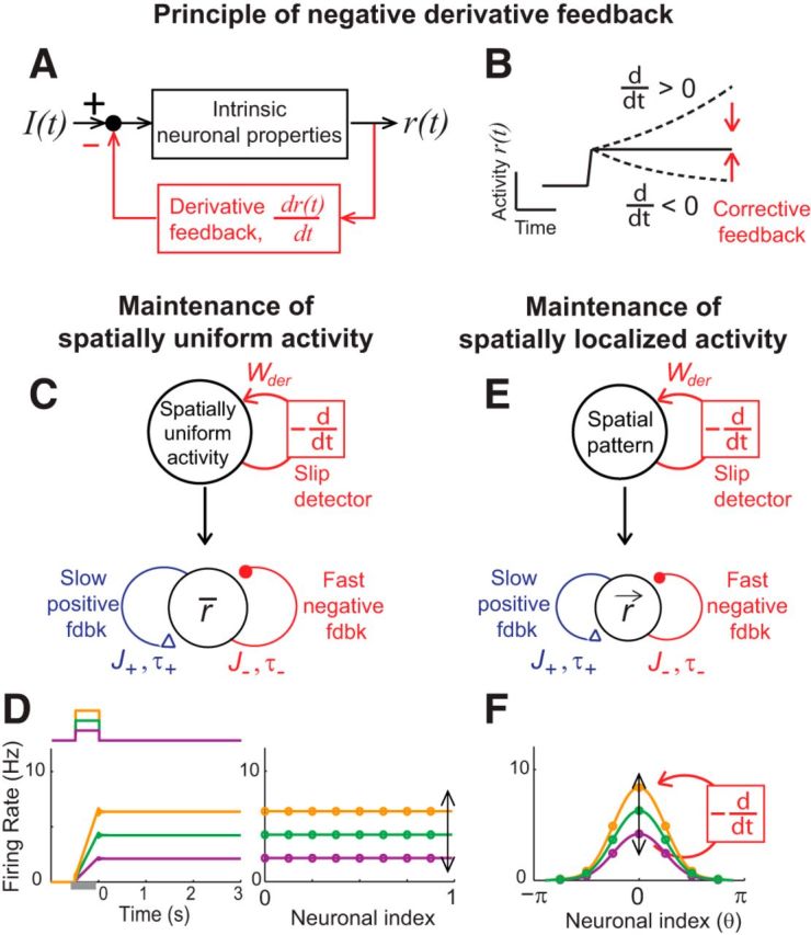
Memory networks with negative-derivative feedback. A, Block diagram illustrating the principle of negative-derivative feedback control for a system with transient external input I(t) and output firing rate r(t). B, A negative-derivative feedback mechanism maintains persistent activity by providing corrective feedback that opposes upward or downward changes in activity. C, Simple black-box model of a neural population with negative-derivative feedback that maintains spatially uniform patterns of persistent activity (top) and simplified network illustrating key components underlying the conditions on the positive and negative feedback pathways for negative-derivative feedback (bottom). D, Time course of average firing rates in spatially uniform negative-derivative feedback networks in response to three example amplitudes of transient stimuli (left) and corresponding maintenance of spatially uniform patterns of activity at different amplitudes (right) during the delay period. E, F, Extension of the mechanism of negative-derivative feedback control to maintaining spatially localized patterns of activity. The basic principles are the same as for the negative-derivative feedback networks for spatially uniform patterns of activity (E), but what negative-derivative feedback detects and corrects is the amplitude of particular spatial patterns of activity (F). In D, the neurons were rank ordered and the neuronal index is the neuron's order number divided by the network size. In F, the neuronal index is the neuron's preferred spatial feature θ.

Mechanistically, this negative-derivative feedback can arise from recurrent network interactions in memory-storing circuits that contain positive and negative feedback pathways (Fig. 2C). When positive feedback mediated by recurrent excitation and negative feedback mediated by recurrent inhibition have equal strength, but positive feedback has slower kinetics, a neuron receives derivative-like recurrent input: the equal-strength positive and negative feedback lead to nearly zero net input during persistent activity, but the faster negative feedback leads to large input that opposes changes in activity whenever activity fluctuates. In spatially uniform networks, the strength of negative-derivative feedback has been shown (Lim and Goldman, 2013) to be proportional to the strength of the balanced positive and negative feedback and the difference in their timescales, so that

where J denotes the strength of the balanced positive and negative feedback pathways, and τ₊ and τ₋ denote the timescales of positive and negative feedback, respectively (Fig. 2C). Thus, when the recurrent synaptic interactions contain strong positive and negative feedback that are balanced in strength (large J) but with slower positive feedback (τ₊ > τ₋), the network temporally integrates its input with long integration time constant τ_eff ≈ W_der, showing step-like activity in response to spatially uniform transient input (Fig. 2D). We note that, although the derivative-feedback mechanism maintains persistent activity by resisting changes in firing rate, this does not keep the system from responding to external inputs as long as these inputs are of the same scale as the recurrent synaptic inputs, which would be expected if the strengths of recurrent and external inputs both scale with population size. Furthermore, external input can transiently imbalance the recurrent excitatory and inhibitory feedback, allowing for more rapid response to external inputs (Lim and Goldman, 2013).

Requirements for negative-derivative feedback in circuits with functionally columnar architecture

Here we describe how the mechanism of negative-derivative feedback described above can be extended to networks that maintain spatially localized patterns of persistent neural activity characteristic of those observed during spatial working memory tasks (Fig. 2E). The basic concept is the same as above, but for spatial working memory, the feature that negative-derivative feedback detects and corrects is a deviation in the amplitude of a particular spatial pattern of activity r⃑ = (r₁,r₂,…,r_n), where r_i is the firing rate of the ith neuron in the network (Fig. 2F). That is, for any maintained spatial pattern r⃑, we require that this activity drives recurrent synaptic interactions containing positive and negative feedback signals of equal strength but with slower kinetics for the positive feedback (Fig. 2E). Below, we show mathematically how these conditions can be met in a spatially structured network and find the conditions on the spatial profile and kinetics of the synaptic connectivity for negative-derivative feedback control.

We consider networks of excitatory and inhibitory populations that store the angular location of a transiently presented spatial cue that must be remembered during a subsequent delay period. Recordings of the persistent activity of spatially selective memory cells identified in such tasks suggest a functionally columnar architecture in which neurons in the same column have similar preferred features of the stimulus (Goldman-Rakic, 1995; Wimmer et al., 2014). To capture this functional organization, we parameterize the activities of the excitatory and inhibitory neurons by their preferred feature θ, which we assume to be uniformly distributed along a ring (Fig. 1). The connection strength between a presynaptic neuron from the jth population with preferred feature θ′and a postsynaptic neuron from the ith population with preferred feature θ is denoted by J_ij(θ,θ′), where i =E or I denotes whether the presynaptic and postsynaptic neurons are part of the excitatory (E) or inhibitory (I) populations. Time constants for these connections similarly are denoted as τ_ij, which is assumed to be independent of θ and θ′ for given population types i and j (Fig. 1).

The core requirements for negative-derivative feedback, a balance between the strengths of the positive and negative feedback pathways and slower positive than negative feedback, impose a tuning condition on the connection strengths J_ij(θ,θ′) and a constraint on the time constants of the connections, τ_ij. To derive the tuning condition on J_ij(θ,θ′), we assume as in most previous models of orientation-selective spatial working memory that the connectivity J_ij(θ,θ′) is translationally invariant, that is, independent of the absolute values of θ and θ′ but dependent on the difference between θ and θ′ as J_ij(θ − θ′) (Ermentrout, 1998; Wang, 2001; Compte, 2006). Furthermore, if the dynamics of the system is linear, Fourier analysis can be used to decompose the spatial activity and recurrent interactions into cosine and sine functions of θ that do not interact with each other (Fig. 3A). In this case, the strengths of the recurrent connections within each Fourier component are denoted by Ĵ_ij(n) and their timescales are given by τ_ij (Fig. 3B, top; see Materials and Methods). However, we note that, although translation invariance and linear dynamics are helpful in building intuition and providing a simple illustration of conditions for negative-derivative feedback, neither of these features are necessary requirements for negative-derivative feedback (see Materials and Methods and Fig. 5 for networks with nonlinear dynamics and Materials and Methods for linear networks without translationally invariant connectivity).

Since the dynamics of each Fourier component are independent, negative-derivative feedback can be achieved independently for each component (Fig. 3A). Specifically, for the nth Fourier component to be governed by negative-derivative feedback, the positive feedback and negative feedback pathways onto this Fourier component should have equal strength, and the positive feedback pathway should have slower kinetics than the negative feedback pathway. This can be accomplished when two conditions are met:

Equation 21 is the condition for balancing positive feedback and negative feedback for the nth Fourier component. The left side of this condition represents the strength of positive feedback in this Fourier component, which is mediated by the E-to-E connection. The right side represents the strength of negative feedback and is mediated by the E-to-I-to-E feedback loop, with normalization of the strength of this loop provided by the I-to-I connection (Fig. 3B, bottom). Equation 22 is the condition for slower positive than negative feedback. The sum τ₊ = τ_EE + τ_II represents the sum of the positive feedback contributions, where τ_II plays the role of a positive feedback time constant because the I-to-I connection inhibits the negative feedback pathway, and this feedback must be slower than the time constant associated with the traversal time around the negative feedback loop τ₋ = τ_EI + τ_IE (Fig. 3B, bottom; see Materials and Methods).

Throughout this paper, we assume that τ_EE is longer than the time constants of the other connections. This assumption is based upon recent experimental observations in prefrontal cortex that found that E-to-E connections are much slower than E-to-I connections, due to a relative prominence of slow NMDA-type synapses (Wang et al., 2008; Wang and Gao, 2009; Rotaru et al., 2011). Thus, because the time constants are independent of the particular Fourier component, Equation 22 is satisfied for all Fourier components.

In contrast, the balance condition, given by Equation 21, can be satisfied independently for each Fourier component. To maintain spatially nonuniform persistent activity across the population, this condition must be satisfied by at least one of the nonconstant Fourier components, and the specific spatial profile of persistent activity observed during the delay period reflects the relative balance of the different components satisfying the balance condition.

Maintenance of spatially modulated activity based on a balance between excitation and inhibition

To illustrate the dynamics of the negative-derivative feedback networks and how they maintain spatially localized patterns of persistent activity, we first consider a simple network that has been structured to receive negative-derivative feedback only in its first cosine component (Fig. 4A). This network's synaptic connectivity profile contained three components, an untuned uniform component of the connectivity, an untuned component with Gaussian connectivity profile, and a tuned component with cosine profile (see Materials and Methods). The network received a spatially localized input of narrow Gaussian profile centered at 0 degrees during a brief cue period, plus a constant background input that was present during both the cue and delay periods (Fig. 4B,C). During the cue presentation and shortly after the offset of the cue, the spatial profile of the network activity had a narrow width that directly followed the spatial profile of the transient input (Fig. 4B, bright horizontal band centered at 0 degrees during the cue period; C, left). However, during the delay period, the activity profile quickly broadened so that only the activity pattern of the first cosine component was maintained (Fig. 4B,C, middle and right). This is because all Fourier components except the first cosine component decayed quickly back to their baseline activity, which was zero for the higher Fourier components and a constant level driven by the tonic background input for the constant component. In contrast, the first cosine component was maintained throughout the delay period by the negative-derivative feedback (Fig. 4B, broad brighter region during delay period; C, middle and right). More generally, this example illustrates that the profile of activity maintained by the network reflects only those components that receive negative-derivative feedback.

A feature of the derivative-feedback networks is that, during the delay period, neurons in the network receive strong excitatory and inhibitory inputs that are closely balanced with each other (Fig. 4D; see Materials and Methods). The cosine component receives a balance of recurrent excitatory and inhibitory synaptic inputs, as required by the balance condition (Fig. 4F). The constant component likewise receives a balance of excitation and inhibition (Fig. 4E). However, this balance is achieved through inclusion of the external background input; the recurrent inputs, in contrast, are dominated by inhibition so that the network does not contain negative-derivative feedback in this component and cannot maintain spatially uniform activity in the absence of background input (data not shown). This reflects that both the excitatory and inhibitory inputs to each neuronal population (but not necessarily the excitatory and inhibitory tuning curves or connectivity, as shown in Fig. 7) are spatially localized and have the same spatial tuning widths.

A close balance between excitatory and inhibitory inputs in memory cells is a distinct feature of negative-derivative feedback. In most previous studies, it has been suggested that spatially localized activity patterns result from excess excitation in high-firing rate neurons and widespread lateral inhibition that stabilizes the bump of activity during the delay period (Ermentrout, 1998; Wang, 2001; Compte, 2006). This leads to inhibitory synaptic inputs onto a postsynaptic cell being more broadly tuned than excitatory inputs in such networks, whereas the spatial tuning of excitatory and inhibitory inputs are similar in negative-derivative feedback networks. Thus, a balance between excitation and inhibition is one prediction of the negative-derivative feedback mechanism that can be tested experimentally (see Discussion).

Location codes, amplitude codes, and neural integration in negative-derivative feedback networks

Traditional spatial working memory models maintain the analog spatial location of a stimulus through stereotyped patterns of network activity centered on the maintained stimulus location, as observed experimentally (Goldman-Rakic, 1995; Wang, 2001). However, a fundamental feature of these models is that the amplitude of the pattern of neuronal activity during the delay period is bistable, either exhibiting untuned background activity or participating in a fixed-amplitude pattern of activity corresponding to the location of the maintained stimulus (Ermentrout, 1998; Wang, 2001; Compte, 2006). Because of this bistability, only the location of the cue can be stored in such networks and, for example, the amplitude or value of the cue cannot be distinguished beyond a binary discrimination.

Negative-derivative feedback networks likewise can maintain an analog spatial location in memory (Fig. 5A) and, as in traditional memory models, this can be achieved by having a translation-invariant network connectivity profile that permits the network to maintain a given spatial pattern of activity centered at any location in the network. However, because the negative-derivative feedback models operate by resisting changes in activity, without regard for the absolute level of activity, they can also maintain analog amplitudes of activity at a given location (Fig. 5B). Thus, these networks can convey information simultaneously about the amplitude and location of a spatial cue (for related examples in the context of optimal Bayesian cue combination and storage and efficient spike-based coding, see Boerlin and Denéve, 2011; Boerlin et al., 2013).

A related feature of the negative-derivative feedback networks is that they can temporally integrate their inputs. Temporal integration is the defining property of neural accumulators that integrate evidence over time (in the sense of calculus) during decision-making processes (Gold and Shadlen, 2007). However, most previous work modeling evidence accumulation has focused primarily upon temporal aspects of this facility, without considering that the accumulated evidence could occur across an analog range of spatial locations. A hallmark of feedback control theory is that the input–output transformation performed by systems with strong negative feedback is approximately equal to the inverse of the function that was fed back. In the case of the negative-derivative feedback networks, the signal that is negatively fed back is the derivative of the activity pattern. Thus, since the functional inverse of a temporal derivative is a temporal integral, these networks output a temporal integral of their inputs. For example, if the inputs are spatially structured, but constant in time, the negative-derivative feedback networks accumulate these signals into a uniformly increasing spatial pattern of activity (Fig. 5C,D). Thus, negative-derivative feedback networks can maintain in memory both the spatial identity of accumulated evidence as well as its running total.

Notably, even in the presence of nonlinearities in intrinsic neuronal dynamics such as thresholds and saturation, negative-derivative feedback networks accumulate and maintain spatially localized activity under the same conditions as in linear networks: a balance between positive and negative feedback, with slower positive feedback than negative feedback, leads to negative-derivative feedback. This occurs even though the Fourier components in a nonlinear network are no longer decoupled and cannot easily be decomposed into independent components (see Materials and Methods). Furthermore, the features of negative-derivative feedback discussed for linear dynamics are maintained under nonlinear dynamics, that is, the networks receive balanced excitation and inhibition during persistent activity (data not shown), and can accumulate and maintain spatially localized patterns of activity at different locations (Fig. 5A, bottom) or at different amplitudes (Fig. 5B–D, bottom; note that at t = 5 s, the neuron with preferred location θ = 0 has approached its absolute maximum firing rate of 100 Hz, demonstrating that in this extreme case the profile does become significantly affected by the nonlinearity).

Maintaining multiple bumps of activity in negative-derivative feedback networks

In the previous sections, we considered networks receiving negative-derivative feedback only in the first cosine component and used this example to illustrate important features of the negative-derivative feedback mechanism–a close balance between excitation and inhibition during persistent activity (Fig. 4D–F) and the ability to encode information both in the location and in the amplitude of spatial patterns of activity (Fig. 5). While these features are hallmarks of negative-derivative feedback networks, the specific activity profile that is maintained during persistent activity is not constrained to simple sinusoids and ultimately is determined by which Fourier components receive negative-derivative feedback. Here, we consider more general networks that receive negative-derivative feedback in all Fourier components and show that such networks can be obtained by a condition analogous to the tuning condition used for the simple cosine example discussed above.

To construct more general networks receiving negative-derivative feedback (Fig. 6A), we consider networks with the same spatial profiles of the excitatory E-to-E and E-to-I connections (Fig. 6B, left) and the same spatial profiles of the inhibitory I-to-E and I-to-I connections (Fig. 6B, right), so that J_ij(θ) = J̃_ijw_j(θ) for i, j = E or I (note that this assumption leads to a simple form of the balance condition, but is not essential to tuning negative-derivative networks more generally). In this case, the Fourier components of the synaptic connectivity profiles are given by Ĵ_ij(n) = J̃_ijŵ_j(n), and the condition for having a balance in strength of positive and negative feedback in a given Fourier mode is given by Ĵ_EE(n)Ĵ_II(n) = J̃_EEJ̃_IIŵ_E(n)ŵ_I(n)∼J̃_EIJ̃_IEŵ_E(n)ŵ_I(n) = Ĵ_EI(n)Ĵ_IE(n), so that J̃_EEJ̃_II ∼ J̃_EIJ̃_IE for large values of J̃_ij for all n. When, in addition, positive feedback is slower than negative feedback (due to a relatively slow combination of self-excitatory and self-inhibitory time constants τ_EE + τ_II > τ_EI + τ_EI), the network interactions provide negative-derivative feedback to all Fourier components.

Unlike the network of Figure 4, which only could maintain broad patterns of activity corresponding to its tuned, first cosine component (Fig. 6C), networks that receive negative-derivative feedback in multiple Fourier components can maintain spatially localized activity with narrower tuning widths that reflect higher order Fourier components. Furthermore, these networks can maintain more general spatial patterns of activity comprised of these different Fourier components, such as activity profiles with multiple bumps (Fig. 6D), which have been suggested as a neural correlate of the storage of multiple items (Laing et al., 2002; Edin et al., 2009; Wei et al., 2012). Thus, networks receiving negative-derivative feedback in multiple Fourier components have a higher memory capacity than those that receive negative-derivative feedback only in a single cosine component. Note, however, that the strength of negative-derivative feedback in each Fourier component, and thus the integration time constant associated with this component, in general will not be the same for all Fourier components, because this strength depends linearly upon the amount of the frequency component that is present within the synaptic connectivity profile. For this reason, the network capacity over a given timescale will in general depend both upon the specific form of the connectivity and the shape of the profile to be maintained so that, for example, networks with broad synaptic connectivity profiles would not be expected to maintain very long-lasting activity for high-frequency components that are minimally represented in their synaptic connectivity. This feature may explain why the long-lasting profiles observed experimentally during spatial working memory tend to be of relatively broad width that likely reflects features of the underlying connectivity profile.

Relation between the profile of synaptic connectivity and tuning widths of activity

Traditional spatial working memory networks require long-range inhibition to maintain the stability of localized patterns of activity in memory (Ermentrout, 1998; Wang, 2001; Compte, 2006). Such long-range inhibition is not prevalent anatomically in cortical networks, although it might be achieved functionally through disynaptic connections (Melchitzky et al., 2001) or through the broadly projecting basket cell subclass of inhibitory interneurons (Markram et al., 2004). In any case, an interesting question is whether long-range inhibition is critical for storing spatial working memory, and what constraints experimental observations may place upon the form of synaptic connectivity.

Unlike traditional models, negative-derivative feedback networks are capable of maintaining spatially localized patterns of activity regardless of the relative widths of excitatory and inhibitory connections (Fig. 7A,C–E). In fact, narrower inhibitory connections are required for our models to generate the experimental observation (Rao et al., 1999, 2000; Constantinidis and Goldman-Rakic, 2002) that inhibitory neurons have broader tuning of activity (after subtracting off any constant baseline) than excitatory neurons (Fig. 7B). When we define “widths” of the activity or connectivity as the spatial spread of the tuned portion after subtracting off any constant, untuned baseline (Constantinidis and Goldman-Rakic, 2002), short-range excitation and long-range inhibition lead to a spatially localized activity profile with the excitatory neurons having broader tuning of activity than the inhibitory neurons (Fig. 7C,F). On the other hand, the reverse relationship of the excitatory and inhibitory synaptic projections, that is, long-range excitation and short-range inhibition (Fig. 7D, or with the addition of nonselective inhibitory projections, Fig. 7E) lead to stable persistent activity with broader tuning of the inhibitory neurons than that of the excitatory neurons (Fig. 7G,H), as seen experimentally (Rao et al., 1999, 2000; Constantinidis and Goldman-Rakic, 2002). In all cases, neurons receive closely balanced excitation and inhibition and thus, the excitatory and inhibitory inputs show the same tuning widths (Fig. 7I–K). This balance of excitation and inhibition with the same spatial tuning is a general feature of negative-derivative feedback networks, since the large amount of excitation and inhibition required for strong derivative feedback must cancel to avoid saturation or total silencing of firing rates.

Thus, in the negative-derivative feedback networks, the relative tuning widths of the excitatory and inhibitory neurons are inversely correlated with the widths of the excitatory and inhibitory synaptic connections (Fig. 7A). This reciprocal relationship between the tuning widths of the neurons and the widths of synaptic projections is a consequence of the balance of excitatory and inhibitory inputs (Fig. 7I–K): because the tuning width of the total excitatory or inhibitory synaptic input onto a neuron is given by a convolution of the synaptic connectivity onto this neuron and the width of the presynaptic neurons' tuning curves, achieving balanced inhibitory and excitatory inputs requires that the experimentally observed broader inhibitory (compared with excitatory) tuning curves be offset by relatively narrower inhibitory synaptic connectivity profiles. This is different from most previous models for spatial working memory, which require broader negative feedback and show no reciprocal relationship between tuning widths of synaptic connectivity and activity profiles. Without different timescales for positive and negative feedback pathways (and, thus, without negative-derivative feedback), narrower negative feedback cannot sustain spatially localized activity (Fig. 8A,E,I,M; see Ermentrout and Cowan, 1980 for a mathematical proof). To stabilize spatially localized activity in such traditional lateral inhibitory models, broader negative feedback than positive feedback is required. This can be achieved either by long-range E-to-I connections (Fig. 8B,F) or long-range I-to-E synaptic connections (Fig. 8C,D,G,H). With broader negative feedback, the excitatory neurons receive broader inhibitory inputs than excitatory inputs (Fig. 8N–P). With no requirement of a close balance between excitation and inhibition, the reciprocal relationship between tuning widths and widths of synaptic projections is not observed in these previous models (Fig. 8J–L). Thus, this reciprocal relationship is a distinct feature of the negative-derivative feedback networks that highlights the mechanism underlying spatial working memory based on balanced excitatory and inhibitory inputs.

Robust memory performance against common perturbations to synaptic weights

A major challenge in short-term memory networks is stably maintaining analog memory representations in the face of perturbations. Although many types of memory networks, including the negative-derivative feedback networks, are quite robust against random noise in synaptic weights that largely can be averaged out across the network or random noise inputs that are filtered out by the slow network dynamics underlying persistent activity, resisting systematic perturbations in weights or intrinsic neuronal response properties has proven to be more challenging. An advantage of negative-derivative networks is that the balance condition that defines these networks is robust against many types of such naturally occurring perturbations. For example, global increases in the intrinsic gains of all neurons, which is equivalent to multiplicatively scaling the strengths of all synaptic connections, does not affect the balance of excitation and inhibition upon which negative-derivative feedback depends. As a result, such perturbations have minimal effect upon the ability of the network to maintain spatially localized persistent activity (Fig. 9A). Conceptually, this is because each neuronal population participates in both positive (through the E-to-E and, effectively, the I-to-I connections) and negative (through E-to-I and I-to-E connections) feedback loops so that such perturbations produce offsetting changes in positive and negative feedback. Quantitatively, this result reflects that the balance condition for derivative-feedback networks is ratiometric, depending only upon the ratio of the synaptic strengths Ĵ_EE(n)Ĵ_II(n)/Ĵ_EI(n)Ĵ_IE(n)∼1 (see Eq. 21). Similarly, examination of this ratiometric condition shows that maintenance of persistent activity with negative-derivative feedback is also robust against global changes in the intrinsic gain of excitatory neurons alone (changes in Ĵ_EE(n) and Ĵ_EI(n); Fig. 9B) or inhibitory neurons alone (changes in Ĵ_IE(n) and Ĵ_II(n); Fig. 9C). Likewise, global changes in excitatory synaptic inputs (Figs. 9E, Fig. 10A,B; changes in Ĵ_EE(n) and Ĵ_IE(n)), inhibitory synaptic inputs (Fig. 9F; changes in Ĵ_EI(n) and Ĵ_II(n)) or all synaptic inputs (Fig. 9D) have minimal effect upon the maintenance of persistent activity, as does loss of a fraction of a subpopulation of neurons, which is equivalent to loss of a fraction of the corresponding excitatory or inhibitory synaptic inputs as in Figure 9D–F.

Furthermore, persistent neural activity in negative-derivative feedback networks is quite robust even against perturbations that occur locally in clusters of neurons with similar preferred spatial locations. To test how well the networks responded to local perturbations, we presented a transient input centered at a location θ = 0 (Fig. 9G–L) and asked how well this item could be maintained in memory following a local perturbation that affected 1/8 of the network. When the perturbation was centered on the preferred location (possibly modeling, for example, effects of attention that changed the gains of neurons triggered by the stimulus), the amplitude of activity increased or decreased mildly for neuronal gain or synaptic weight increases or decreases, respectively, but the time course of persistent activity was only mildly affected (Fig. 10C,D), with the change in time constant approximately linearly related to the perturbation size (data not shown). When the perturbation was located on the flanks of the presented stimulus location (Fig. 9G–L; black bar along x-axis), activity was again maintained persistently in time (data not shown), although there was a small warping of the Gaussian-shaped bump that reflected that the perturbation disrupted the translation-invariant form of the network's structure. Thus, in this case, the perturbation would slightly bias the observation of the cue location if the readout of the network activity remained the same as before the perturbation. However, because the local perturbation does not affect the balance of positive and negative feedback that maintains persistent activity, the cue would remain in memory and, if the perturbation were continually present, a change in network readout could in principle learn to compensate for the changes in shape of the maintained activity profile.

The negative-derivative feedback networks are not robust against all forms of perturbations, in particular those that break the balance between excitation and inhibition that underlies the balance in strength of the positive and negative feedback components of negative-derivative feedback. For example, global or local perturbations in specific excitatory pathways, such as the E-to-E pathways that are dominated by NMDA-type synapses, do disrupt persistent activity (Fig. 10E–H). This is because NMDA-mediated currents are stronger at E-to-E than E-to-I connections (Wang et al., 2008; Wang and Gao, 2009; Rotaru et al., 2011); therefore their disruption imbalances the positive and negative feedback pathways, consistent with recent experimental observations of lack of robustness of working memory to pharmacological blockade of NMDA receptors (Wang et al., 2013). The disruption of persistent activity under such perturbations can be quantified by changes of the time constant of decay of activity at the perturbed location, τ_eff. As the ratio between the strengths of the positive and negative feedback J_pos/J_neg deviates from 1, τ_eff decreases inversely proportional to 1 − J_pos/J_neg (Fig. 10I,J). Thus, while many common perturbations such as loss of neurons, changes in intrinsic neuronal gains, or uniform changes in synaptic strengths maintain J_pos/J_neg close to 1 (Fig. 10I, dashed diagonal line), the negative-derivative feedback networks are susceptible to perturbations that break the tuning of J_pos/J_neg ∼ 1 (Fig. 10I, off-diagonal portions).

We note that the lack of robustness to perturbations that disrupt the excitatory–inhibitory balance in our model is different from the behavior observed in previous lateral inhibition models that require rough but not exact balance between excitation and inhibition and therefore exhibit robust memory performance across a wider range of perturbations in connectivity. For example, mild perturbations of the strength of the E-to-E connection alone or the E-to-I or I-to-E connections alone do not affect the memory performance of lateral inhibition models (Camperi and Wang, 1998; Hansel and Sompolinsky, 1998). However, in these models, the spatial patterns of activity can be maintained only at a fixed amplitude, rather than the graded range of amplitudes that can be sustained in models based upon derivative feedback. Thus, the more stringent tuning conditions on synaptic connections in the negative-derivative feedback networks reflects a trade-off between robustness to excitatory–inhibitory imbalance and being able to encode the amplitude of spatial patterns of activity and temporally integrate the strength of inputs.

Irregular firing activity during persistent activity

A characteristic feature of persistent neural activity during spatial working memory tasks is the irregular, Poisson-like nature of the firing activity (Compte et al., 2003). This has been a challenge for most previous spatial working memory models because, in these models, elevated persistent activity is maintained by a constant, suprathreshold excitatory drive that causes relatively regular persistent firing unless large external sources of noise are included (Barbieri and Brunel, 2008; but see Barbieri and Brunel, 2007; Renart et al., 2007; Roudi and Latham, 2007; Lundqvist et al., 2010; Boerlin and Denéve, 2011; Mongillo et al., 2012; Boerlin et al., 2013; Hansel and Mato, 2013). In contrast, negative-derivative feedback networks operate in a regime of closely balanced excitation and inhibition, so that the mean synaptic input is subthreshold and firing is driven largely by fluctuations that lead to a high coefficient of variation of the interspike intervals (Shadlen and Newsome, 1994; van Vreeswijk and Sompolinsky, 1996; Amit and Brunel, 1997; Troyer and Miller, 1997; Renart et al., 2007; Roudi and Latham, 2007). This spike-train irregularity was shown previously in spatially uniform negative-derivative feedback models (Lim and Goldman, 2013). Here, we show that the same result occurs in negative-derivative feedback networks with spatial structure.

We constructed spiking network models with the same columnar structure as in the firing rate models (Fig. 1). Each column consisted of excitatory and inhibitory integrate-and-fire neurons with similar preferred spatial features, and the connectivity between neurons within and across the columns was random and sparse (van Vreeswijk and Sompolinsky, 1996). For connected neurons, the strength of synaptic connections was assumed to be a Gaussian function of the difference between the preferred features of the presynaptic and postsynaptic neurons (Fig. 6B), and the strengths of the excitatory and inhibitory connections on average were set to satisfy the balance condition of Equation 21. However, we note that the connection strengths onto individual neurons were not precisely balanced and were heterogeneous due to the sparse and random connectivity of the network. Inhibitory currents were mediated by GABA_A receptors and recurrent excitatory currents were mediated by a mixture of AMPA and NMDA receptors, with a greater proportion of and slower kinetics of NMDA receptors in the excitatory feedback pathways (Wang et al., 2008; Wang and Gao, 2009; Rotaru et al., 2011). The networks receive spatially patterned input during the stimulus presentation, but no input during the delay period.

As in the firing rate models, these spiking networks implementing negative-derivative feedback showed spatially tuned persistent activity encoding the cue location of the transiently presented stimulus (Fig. 11B). Due to the balance between excitation and inhibition, the neuronal spike trains were highly irregular during the delay period (Fig. 11C,D,F,G). Quantitative analysis of the spike-train irregularity using the local coefficient of variation CV₂ (see Materials and Methods) found that the model distributions were similar to those observed experimentally in memory cells receiving preferred cue or nonpreferred cue stimuli (Fig. 11A, experiments; E,H, model). Thus, the principle of negative-derivative feedback also is applicable to spiking networks and networks incorporating this principle can reproduce salient properties of biological working memory networks such as spatially tuned delay period activity and irregular firing.

Discussion

Here we suggest a new model for spatial working memory based on negative-derivative feedback control. When recurrent inhibition and excitation are balanced, and the feedback pathways mediating positive feedback are slower than those mediating negative feedback, we have shown how a network with functionally columnar architecture can maintain analog amplitude signals corresponding to any spatial location. Furthermore, we have demonstrated that these negative-derivative feedback networks can temporally integrate their inputs, thus showing how accumulation of sensory input can be performed in a spatially specific manner. Given that recent experiments in frontal cortex suggest a balance of inhibition and excitation (Shu et al., 2003; Haider et al., 2006) as well as differential kinetics in the E-to-E versus E-to-I pathways mediating positive versus negative feedback (Wang et al., 2008; Wang and Gao, 2009; Rotaru et al., 2011), this suggests that negative-derivative feedback may serve as a fundamental principle underlying the accumulation and storage of signals in spatial working memory.

Comparison to network models with lateral inhibition and experimental predictions

A “Mexican-hat” network architecture with a broader range of inhibitory interactions than excitatory interactions between neurons is prevalent in cortical circuit models that generate spatial patterns of activity for working memory (Ermentrout, 1998; Wang, 2001; Compte, 2006). Compared with most previous network models with functionally long-range inhibition, negative-derivative feedback networks exhibit several distinct features. First, negative-derivative feedback networks do not require long-range inhibition. Second, they receive massive amounts of excitatory and inhibitory inputs that are closely balanced. Third, this close balance between excitation and inhibition leads to irregular firing activity during the delay period, consistent with experimental observations in cortical memory circuits (Compte et al., 2003). Fourth, negative-derivative feedback networks can encode information about a transient stimulus not only in the location but also in the amplitude of its spatial patterns of activity and, in principle, can maintain arbitrary spatial patterns of activity (see also Carroll et al., 2014 for a special network with fast inhibitory neurons and tuning of both the form of neuronal response nonlinearity and connectivity to allow graded-amplitude spatial patterns of activity to be maintained with long-range inhibition).

The negative-derivative feedback networks require a tight tuning condition on network connectivity to have positive and negative feedback of equal strengths. This tuning condition is more stringent than that of the previous lateral inhibition models, which require only rough balance between the strengths of positive and negative feedback (Camperi and Wang, 1998; Hansel and Sompolinsky, 1998). However, in such systems, spatial patterns of activity can be maintained only at a fixed amplitude and thus, the strictness of the tuning condition in derivative feedback models can be considered as a trade-off with being able to maintain activity across a graded range of levels and to temporally integrate inputs. Somewhat mitigating the strictness of this tuning condition is the fact that it applies only to the average connectivity of the different populations and does not require that the tuning be exact for each individual neuron. As shown in Figure 9, this tuning condition may be preserved following many natural perturbations, such as changes in intrinsic or synaptic gains or loss of subpopulations of neurons that occur globally or locally in the circuits. On a slower timescale, recent work suggests that the excitatory–inhibitory balance in cortical cells may be actively maintained by homeostatic mechanisms (Liu, 2004; Vogels et al., 2011), or may be achieved gradually through the developmental refinement of synaptic connections (Tao and Poo, 2005). Thus, the balance of inhibition and excitation required for derivative-feedback memory networks may be quite robust in normal situations.

The distinct features of our model provide testable predictions. First, negative-derivative feedback networks predict similar spatial tuning between excitatory and inhibitory inputs due to a close balance between them (Figs. 4D, 7I–K). Experimentally, a balance between strong excitatory and inhibitory synaptic inputs (Shu et al., 2003; Haider et al., 2006) and co-tuning between them (Destexhe et al., 2003; Wehr and Zador, 2003; Priebe and Ferster, 2005; Rudolph et al., 2007) have been observed in cortical neurons, although the ultimate test, intracellular recordings of memory cells in a behaving animal, has yet to be performed and currently stands as a prediction of our model. Second, perturbations in specific synaptic pathways–such as blockade of excitatory or inhibitory transmission exclusively onto excitatory or inhibitory neurons that break the balance between excitation and inhibition–would cause more severe impairments of persistent activity than completely silencing a subset of excitatory or inhibitory neurons. Consistent with this prediction, a recent experiment blocking slow NMDA-mediated currents that are especially prominent in the pyramidal-to-pyramidal (E-to-E) connections of prefrontal cortex (Wang et al., 2013) did lead to strong impairments in working memory performance. Third, the balance condition between excitation and inhibition provides negative correlation between the relative tuning widths of the excitatory and inhibitory neurons and the widths of the excitatory and inhibitory synaptic connections, such that if the inhibitory synaptic projection is shorter range, the balance in inputs is preserved under broader tuning of the inhibitory neurons. Finally, we note that it is possible that different mechanisms are used in networks that maintain graded representations from those that maintain only spatial location information, so experiments designed to test these predictions ideally should be performed using paradigms that require both the spatial location and amplitude (or duration for integrators) of stimuli to be encoded.

Irregular firing statistics based on balanced excitation and inhibition

The irregular firing activity observed during working memory performance (Compte et al., 2003) provides indirect support for a balance between excitation and inhibition in the neurons supporting this activity. This balance has been a challenge to achieve in most models of working memory, because these models depend upon stronger excitation than inhibition to maintain elevated firing rates, and such imbalanced excitation tends to lead to regular patterns of neuronal firing (Barbieri and Brunel, 2008). In contrast, negative-derivative feedback networks inherently depend upon a balance of inhibition and excitation throughout an analog range of firing rates, leading to irregular firing at all rates.

To account for irregular spiking activity during a delay period, recent works have suggested bistable memory circuits based on balanced excitation and inhibition. These balanced networks can maintain elevated (UP) states through neuronal nonlinearities (Barbieri and Brunel, 2007; Renart et al., 2007; Roudi and Latham, 2007; Lundqvist et al., 2010) or through synaptic nonlinearities associated with short-term synaptic plasticity (Mongillo et al., 2012; Hansel and Mato, 2013). However, with the exception of Hansel and Mato (2013), these networks used identical time constants for positive and negative feedback pathways so that they do not contain negative-derivative feedback, are not able to maintain a graded range of persistent activity and perform temporal integration, and can be distinguished from the negative-derivative feedback networks by their essential dependence upon lateral inhibition to stabilize spatially localized persistent activity (Fig. 8).

Like our networks, the spatial working memory networks of Hansel and Mato (2013) show similar tuning of excitatory and inhibitory inputs and contain an asymmetric ratio of NMDA/AMPA currents in the E-to-E versus E-to-I connections, resulting in slower positive than negative feedback. Thus, these networks also may contain a derivative-feedback signal that contributes to their robustness, and an interesting question is whether the principle of negative-derivative feedback could be useful in bistable, as well as analog, spatial memory networks. In separate work, networks built upon the principle of optimal inference of external inputs and efficient spike-based coding can maintain analog-valued amplitudes of irregular persistent activity (Boerlin and Denéve, 2011; Boerlin et al., 2013). These networks require balanced excitation and inhibition with slower excitation, and thus likely also depend upon a large negative-derivative feedback component, suggesting that the principle of negative-derivative feedback control may be derived independently from the theory of Bayesian inference and spike-based coding.

Memory capacity of negative-derivative networks

A distinctive feature of the negative-derivative feedback networks is that they can maintain spatially localized activity of different amplitudes as well as at different locations (Fig. 5). This could be useful in modulating network response as a function of attention (Reynolds and Chelazzi, 2004) or reward (Schultz et al., 1993; Watanabe, 1996; Leon and Shadlen, 1999; Amemori and Sawaguchi, 2006). Alternatively, simultaneously being able to vary amplitude and location could be useful in encoding quantities such as the color of a patch that can vary in an analog manner in both spatial and nonspatial dimensions (Luck and Vogel, 1997; Zhang and Luck, 2008), or in accumulating the value of a single quantity over time (Gold and Shadlen, 2007) in a spatially specific manner. However, we note that the ability to integrate external inputs makes negative-derivative feedback networks relatively more sensitive to noisy or interfering input present during memory performance. To enhance the signal-to-noise ratio of negative-derivative feedback networks, additional mechanisms may be required to suppress external inputs during memory performance, for example, by dopamine regulation that is triggered with the onset of task-related input (Sawaguchi et al., 1988; Durstewitz et al., 1999).

Negative-derivative feedback networks also can maintain activities with multiple bumps when negative-derivative feedback is present in higher order Fourier components. Previous studies have suggested that the width of recurrent excitatory connections is a critical factor determining the maximal number of items that can be stored in the network (Edin et al., 2009; Wei et al., 2012). On the other hand, the memory capacity of negative-derivative feedback networks is determined by the amount of negative-derivative feedback in higher order Fourier components, and thus the width of both the excitatory and inhibitory connections affects memory capacity. Since storing more items requires the maintenance of narrower, higher frequency-containing patterns, this may provide a fundamental constraint on the forms of synaptic connectivity in memory networks. Further work is needed to explore the relationship between memory capacity and connectivity structure, and to compare the performance of negative-derivative feedback networks with that of previous network models.

References

- Amemori K, Sawaguchi T. Contrasting effects of reward expectation on sensory and motor memories in primate prefrontal neurons. Cereb Cortex. 2006;16:1002–1015. doi: 10.1093/cercor/bhj042. [DOI] [PubMed] [Google Scholar]
- Amit DJ, Brunel N. Model of global spontaneous activity and local structured activity during delay periods in the cerebral cortex. Cereb Cortex. 1997;7:237–252. doi: 10.1093/cercor/7.3.237. [DOI] [PubMed] [Google Scholar]
- Barbieri F, Brunel N. Irregular persistent activity induced by synaptic excitatory feedback. Front Comput Neurosci. 2007;1:5. doi: 10.3389/neuro.10.005.2007. [DOI] [PMC free article] [PubMed] [Google Scholar]
- Barbieri F, Brunel N. Can attractor network models account for the statistics of firing during persistent activity in prefrontal cortex? Front Neurosci. 2008;2:114–122. doi: 10.3389/neuro.01.003.2008. [DOI] [PMC free article] [PubMed] [Google Scholar]
- Ben-Yishai R, Bar-Or RL, Sompolinsky H. Theory of orientation tuning in visual cortex. Proc Natl Acad Sci U S A. 1995;92:3844–3848. doi: 10.1073/pnas.92.9.3844. [DOI] [PMC free article] [PubMed] [Google Scholar]
- Boerlin M, Denève S. Spike-based population coding and working memory. PLoS Comput Biol. 2011;7:e1001080. doi: 10.1371/journal.pcbi.1001080. [DOI] [PMC free article] [PubMed] [Google Scholar]
- Boerlin M, Machens CK, Denève S. Predictive coding of dynamical variables in balanced spiking networks. PLoS Comput Biol. 2013;9:e1003258. doi: 10.1371/journal.pcbi.1003258. [DOI] [PMC free article] [PubMed] [Google Scholar]
- Braitenberg V, Schüz A. Cortex: statistics and geometry of neuronal connectivity. Ed 2. New York: Springer; 1998. [Google Scholar]
- Camperi M, Wang XJ. A model of visuospatial working memory in prefrontal cortex: recurrent network and cellular bistability. J Comput Neurosci. 1998;5:383–405. doi: 10.1023/A:1008837311948. [DOI] [PubMed] [Google Scholar]
- Carroll S, Josic K, Kilpatrick ZP. Encoding certainty in bump attractors. J Comput Neurosci. 2013 doi: 10.1007/s10827-013-0486-0. doi: 10.1007/s10827-013-0486-0. Advance online publication. [DOI] [PubMed] [Google Scholar]
- Chafee MV, Goldman-Rakic PS. Matching patterns of activity in primate prefrontal area 8a and parietal area 7ip neurons during a spatial working memory task. J Neurophysiol. 1998;79:2919–2940. doi: 10.1152/jn.1998.79.6.2919. [DOI] [PubMed] [Google Scholar]
- Compte A. Computational and in vitro studies of persistent activity: edging towards cellular and synaptic mechanisms of working memory. Neuroscience. 2006;139:135–151. doi: 10.1016/j.neuroscience.2005.06.011. [DOI] [PubMed] [Google Scholar]
- Compte A, Constantinidis C, Tegner J, Raghavachari S, Chafee MV, Goldman-Rakic PS, Wang XJ. Temporally irregular mnemonic persistent activity in prefrontal neurons of monkeys during a delayed response task. J Neurophysiol. 2003;90:3441–3454. doi: 10.1152/jn.00949.2002. [DOI] [PubMed] [Google Scholar]
- Constantinidis C, Goldman-Rakic PS. Correlated discharges among putative pyramidal neurons and interneurons in the primate prefrontal cortex. J Neurophysiol. 2002;88:3487–3497. doi: 10.1152/jn.00188.2002. [DOI] [PubMed] [Google Scholar]
- Constantinidis C, Steinmetz MA. Neuronal activity in posterior parietal area 7a during the delay periods of a spatial memory task. J Neurophysiol. 1996;76:1352–1355. doi: 10.1152/jn.1996.76.2.1352. [DOI] [PubMed] [Google Scholar]
- Destexhe A, Rudolph M, Paré D. The high-conductance state of neocortical neurons in vivo. Nat Rev Neurosci. 2003;4:739–751. doi: 10.1038/nrn1198. [DOI] [PubMed] [Google Scholar]
- Douglas RJ, Martin KA. Neuronal circuits of the neocortex. Annu Rev Neurosci. 2004;27:419–451. doi: 10.1146/annurev.neuro.27.070203.144152. [DOI] [PubMed] [Google Scholar]
- Durstewitz D, Kelc M, Güntürkün O. A neurocomputational theory of the dopaminergic modulation of working memory functions. J Neurosci. 1999;19:2807–2822. doi: 10.1523/JNEUROSCI.19-07-02807.1999. [DOI] [PMC free article] [PubMed] [Google Scholar]
- Edin F, Klingberg T, Johansson P, McNab F, Tegnér J, Compte A. Mechanism for top-down control of working memory capacity. Proc Natl Acad Sci U S A. 2009;106:6802–6807. doi: 10.1073/pnas.0901894106. [DOI] [PMC free article] [PubMed] [Google Scholar]
- Ermentrout B. Neural networks as spatio-temporal pattern-forming systems. Rep Prog Phys. 1998;61:353–430. doi: 10.1088/0034-4885/61/4/002. [DOI] [Google Scholar]
- Ermentrout B, Cowan JD. Large scale spatially organized activity in neural nets. SIAM J Appl Math. 1980;38:1–21. doi: 10.1137/0138001. [DOI] [Google Scholar]
- Folland GB. Fourier analysis and its applications. Providence, RI: American Mathematical Society; 2009. [Google Scholar]
- Funahashi S, Bruce CJ, Goldman-Rakic PS. Mnemonic coding of visual space in the monkey's dorsolateral prefrontal cortex. J Neurophysiol. 1989;61:331–349. doi: 10.1152/jn.1989.61.2.331. [DOI] [PubMed] [Google Scholar]
- Gold JI, Shadlen MN. The neural basis of decision making. Annu Rev Neurosci. 2007;30:535–574. doi: 10.1146/annurev.neuro.29.051605.113038. [DOI] [PubMed] [Google Scholar]
- Goldman-Rakic PS. Cellular basis of working memory. Neuron. 1995;14:477–485. doi: 10.1016/0896-6273(95)90304-6. [DOI] [PubMed] [Google Scholar]
- Haider B, McCormick DA. Rapid neocortical dynamics: cellular and network mechanisms. Neuron. 2009;62:171–189. doi: 10.1016/j.neuron.2009.04.008. [DOI] [PMC free article] [PubMed] [Google Scholar]
- Haider B, Duque A, Hasenstaub AR, McCormick DA. Neocortical network activity in vivo is generated through a dynamic balance of excitation and inhibition. J Neurosci. 2006;26:4535–4545. doi: 10.1523/JNEUROSCI.5297-05.2006. [DOI] [PMC free article] [PubMed] [Google Scholar]
- Hansel D, Mato G. Short-term plasticity explains irregular persistent activity in working memory tasks. J Neurosci. 2013;33:133–149. doi: 10.1523/JNEUROSCI.3455-12.2013. [DOI] [PMC free article] [PubMed] [Google Scholar]
- Hansel D, Sompolinsky H. Modeling feature selectivity in local cortical circuits. In: Koch C, Segev I, editors. Methods in neuronal modeling: from synapses to networks. Ed 2. Cambridge, MA: MIT; 1998. [Google Scholar]
- Hansel D, Mato G, Meunier C, Neltner L. On numerical simulations of integrate-and-fire neural networks. Neural Comput. 1998;10:467–483. doi: 10.1162/089976698300017845. [DOI] [PubMed] [Google Scholar]
- Holt GR, Softky WR, Koch C, Douglas RJ. Comparison of discharge variability in vitro and in vivo in cat visual cortex neurons. J Neurophysiol. 1996;75:1806–1814. doi: 10.1152/jn.1996.75.5.1806. [DOI] [PubMed] [Google Scholar]
- Laing CR, Troy WC, Gutkin B, Ermentrout GB. Multiple bumps in a neuronal model of working memory. SIAM J Appl Math. 2002;63:62–97. doi: 10.1137/S0036139901389495. [DOI] [Google Scholar]
- Leon MI, Shadlen MN. Effect of expected reward magnitude on the response of neurons in the dorsolateral prefrontal cortex of the macaque. Neuron. 1999;24:415–425. doi: 10.1016/S0896-6273(00)80854-5. [DOI] [PubMed] [Google Scholar]
- Lim S, Goldman MS. Balanced cortical microcircuitry for maintaining information in working memory. Nat Neurosci. 2013;16:1306–1314. doi: 10.1038/nn.3492. [DOI] [PMC free article] [PubMed] [Google Scholar]
- Liu G. Local structural balance and functional interaction of excitatory and inhibitory synapses in hippocampal dendrites. Nat Neurosci. 2004;7:373–379. doi: 10.1038/nn1206. [DOI] [PubMed] [Google Scholar]
- Luck SJ, Vogel EK. The capacity of visual working memory for features and conjunctions. Nature. 1997;390:279–281. doi: 10.1038/36846. [DOI] [PubMed] [Google Scholar]
- Lundqvist M, Compte A, Lansner A. Bistable, irregular firing and population oscillations in a modular attractor memory network. PLoS Comput Biol. 2010;6:e1000803. doi: 10.1371/journal.pcbi.1000803. [DOI] [PMC free article] [PubMed] [Google Scholar]
- Markram H, Toledo-Rodriguez M, Wang Y, Gupta A, Silberberg G, Wu C. Interneurons of the neocortical inhibitory system. Nat Rev Neurosci. 2004;5:793–807. doi: 10.1038/nrn1519. [DOI] [PubMed] [Google Scholar]
- McCormick DA, Connors BW, Lighthall JW, Prince DA. Comparative electrophysiology of pyramidal and sparsely spiny stellate neurons of the neocortex. J Neurophysiol. 1985;54:782–806. doi: 10.1152/jn.1985.54.4.782. [DOI] [PubMed] [Google Scholar]
- Melchitzky DS, González-Burgos G, Barrionuevo G, Lewis DA. Synaptic targets of the intrinsic axon collaterals of supragranular pyramidal neurons in monkey prefrontal cortex. J Comp Neurol. 2001;430:209–221. doi: 10.1002/1096-9861(20010205)430:2<209::AID-CNE1026>3.0.CO%3B2-%23. [DOI] [PubMed] [Google Scholar]
- Mongillo G, Hansel D, van Vreeswijk C. Bistability and spatiotemporal irregularity in neuronal networks with nonlinear synaptic transmission. Phys Rev Lett. 2012;108:158101. doi: 10.1103/PhysRevLett.108.158101. [DOI] [PubMed] [Google Scholar]
- Nise NS. Control systems engineering. Ed 4. New York: Wiley; 2004. [Google Scholar]
- Priebe NJ, Ferster D. Direction selectivity of excitation and inhibition in simple cells of the cat primary visual cortex. Neuron. 2005;45:133–145. doi: 10.1016/j.neuron.2004.12.024. [DOI] [PubMed] [Google Scholar]
- Rao SG, Williams GV, Goldman-Rakic PS. Isodirectional tuning of adjacent interneurons and pyramidal cells during working memory: evidence for microcolumnar organization in PFC. J Neurophysiol. 1999;81:1903–1916. doi: 10.1152/jn.1999.81.4.1903. [DOI] [PubMed] [Google Scholar]
- Rao SG, Williams GV, Goldman-Rakic PS. Destruction and creation of spatial tuning by disinhibition: GABA(A) blockade of prefrontal cortical neurons engaged by working memory. J Neurosci. 2000;20:485–494. doi: 10.1523/JNEUROSCI.20-01-00485.2000. [DOI] [PMC free article] [PubMed] [Google Scholar]
- Renart A, Moreno-Bote R, Wang XJ, Parga N. Mean-driven and fluctuation-driven persistent activity in recurrent networks. Neural Comput. 2007;19:1–46. doi: 10.1162/neco.2007.19.1.1. [DOI] [PubMed] [Google Scholar]
- Reynolds JH, Chelazzi L. Attentional modulation of visual processing. Annu Rev Neurosci. 2004;27:611–647. doi: 10.1146/annurev.neuro.26.041002.131039. [DOI] [PubMed] [Google Scholar]
- Rotaru DC, Yoshino H, Lewis DA, Ermentrout GB, Gonzalez-Burgos G. Glutamate receptor subtypes mediating synaptic activation of prefrontal cortex neurons: relevance for schizophrenia. J Neurosci. 2011;31:142–156. doi: 10.1523/JNEUROSCI.1970-10.2011. [DOI] [PMC free article] [PubMed] [Google Scholar]
- Roudi Y, Latham PE. A balanced memory network. PLoS Comput Biol. 2007;3:1679–1700. doi: 10.1371/journal.pcbi.0030141. [DOI] [PMC free article] [PubMed] [Google Scholar]
- Rudolph M, Pospischil M, Timofeev I, Destexhe A. Inhibition determines membrane potential dynamics and controls action potential generation in awake and sleeping cat cortex. J Neurosci. 2007;27:5280–5290. doi: 10.1523/JNEUROSCI.4652-06.2007. [DOI] [PMC free article] [PubMed] [Google Scholar]
- Salin PA, Prince DA. Spontaneous GABAA receptor-mediated inhibitory currents in adult rat somatosensory cortex. J Neurophysiol. 1996;75:1573–1588. doi: 10.1152/jn.1996.75.4.1573. [DOI] [PubMed] [Google Scholar]
- Sawaguchi T, Matsumura M, Kubota K. Dopamine enhances the neuronal activity of spatial short-term memory task in the primate prefrontal cortex. Neurosci Res. 1988;5:465–473. doi: 10.1016/0168-0102(88)90030-2. [DOI] [PubMed] [Google Scholar]
- Schultz W, Apicella P, Ljungberg T. Responses of monkey dopamine neurons to reward and conditioned stimuli during successive steps of learning a delayed response task. J Neurosci. 1993;13:900–913. doi: 10.1523/JNEUROSCI.13-03-00900.1993. [DOI] [PMC free article] [PubMed] [Google Scholar]
- Shadlen MN, Newsome WT. Noise, neural codes and cortical organization. Curr Opin Neurobiol. 1994;4:569–579. doi: 10.1016/0959-4388(94)90059-0. [DOI] [PubMed] [Google Scholar]
- Shu Y, Hasenstaub A, McCormick DA. Turning on and off recurrent balanced cortical activity. Nature. 2003;423:288–293. doi: 10.1038/nature01616. [DOI] [PubMed] [Google Scholar]
- Tao HW, Poo MM. Activity-dependent matching of excitatory and inhibitory inputs during refinement of visual receptive fields. Neuron. 2005;45:829–836. doi: 10.1016/j.neuron.2005.01.046. [DOI] [PubMed] [Google Scholar]
- Troyer TW, Miller KD. Physiological gain leads to high ISI variability in a simple model of a cortical regular spiking cell. Neural Comput. 1997;9:971–983. doi: 10.1162/neco.1997.9.5.971. [DOI] [PubMed] [Google Scholar]
- van Vreeswijk C, Sompolinsky H. Chaos in neuronal networks with balanced excitatory and inhibitory activity. Science. 1996;274:1724–1726. doi: 10.1126/science.274.5293.1724. [DOI] [PubMed] [Google Scholar]
- van Vreeswijk C, Sompolinsky H. Chaotic balanced state in a model of cortical circuits. Neural Comput. 1998;10:1321–1371. doi: 10.1162/089976698300017214. [DOI] [PubMed] [Google Scholar]
- Vogels TP, Sprekeler H, Zenke F, Clopath C, Gerstner W. Inhibitory plasticity balances excitation and inhibition in sensory pathways and memory networks. Science. 2011;334:1569–1573. doi: 10.1126/science.1211095. [DOI] [PubMed] [Google Scholar]
- Wang HX, Gao WJ. Cell type-specific development of NMDA receptors in the interneurons of rat prefrontal cortex. Neuropsychopharmacology. 2009;34:2028–2040. doi: 10.1038/npp.2009.20. [DOI] [PMC free article] [PubMed] [Google Scholar]
- Wang H, Stradtman GG, 3rd, Wang XJ, Gao WJ. A specialized NMDA receptor function in layer 5 recurrent microcircuitry of the adult rat prefrontal cortex. Proc Natl Acad Sci U S A. 2008;105:16791–16796. doi: 10.1073/pnas.0804318105. [DOI] [PMC free article] [PubMed] [Google Scholar]
- Wang M, Yang Y, Wang CJ, Gamo NJ, Jin LE, Mazer JA, Morrison JH, Wang XJ, Arnsten AF. NMDA receptors subserve persistent neuronal firing during working memory in dorsolateral prefrontal cortex. Neuron. 2013;77:736–749. doi: 10.1016/j.neuron.2012.12.032. [DOI] [PMC free article] [PubMed] [Google Scholar]
- Wang XJ. Synaptic reverberation underlying mnemonic persistent activity. Trends Neurosci. 2001;24:455–463. doi: 10.1016/S0166-2236(00)01868-3. [DOI] [PubMed] [Google Scholar]
- Watanabe M. Reward expectancy in primate prefrontal neurons. Nature. 1996;382:629–632. doi: 10.1038/382629a0. [DOI] [PubMed] [Google Scholar]
- Wehr M, Zador AM. Balanced inhibition underlies tuning and sharpens spike timing in auditory cortex. Nature. 2003;426:442–446. doi: 10.1038/nature02116. [DOI] [PubMed] [Google Scholar]
- Wei Z, Wang XJ, Wang DH. From distributed resources to limited slots in multiple-item working memory: a spiking network model with normalization. J Neurosci. 2012;32:11228–11240. doi: 10.1523/JNEUROSCI.0735-12.2012. [DOI] [PMC free article] [PubMed] [Google Scholar]
- Wilson HR. Spikes, decisions, and actions. New York: Oxford UP; 1999. [Google Scholar]
- Wimmer K, Nykamp DQ, Constantinidis C, Compte A. Bump attractor dynamics in prefrontal cortex explains behavioral precision in spatial working memory. Nat Neurosci. 2014;17:431–439. doi: 10.1038/nn.3645. [DOI] [PubMed] [Google Scholar]
- Xiang Z, Huguenard JR, Prince DA. GABAA receptor-mediated currents in interneurons and pyramidal cells of rat visual cortex. J Physiol. 1998;506:715–730. doi: 10.1111/j.1469-7793.1998.715bv.x. [DOI] [PMC free article] [PubMed] [Google Scholar]
- Zhang W, Luck SJ. Discrete fixed-resolution representations in visual working memory. Nature. 2008;453:233–235. doi: 10.1038/nature06860. [DOI] [PMC free article] [PubMed] [Google Scholar]