

Abstract.
In continuous-wave near-infrared spectroscopy (CW-NIRS), changes in the concentration of oxyhemoglobin and deoxyhemoglobin can be calculated by solving a set of linear equations from the modified Beer-Lambert Law. Cross-talk error in the calculated hemodynamics can arise from inaccurate knowledge of the wavelength-dependent differential path length factor (DPF). We apply the extended Kalman filter (EKF) with a dynamical systems model to calculate relative concentration changes in oxy- and deoxyhemoglobin while simultaneously estimating relative changes in DPF. Results from simulated and experimental CW-NIRS data are compared with results from a weighted least squares (WLSQ) method. The EKF method was found to effectively correct for artificially introduced errors in DPF and to reduce the cross-talk error in simulation. With experimental CW-NIRS data, the hemodynamic estimates from EKF differ significantly from the WLSQ (). The cross-correlations among residuals at different wavelengths were found to be significantly reduced by the EKF method compared to WLSQ in three physiologically relevant spectral bands 0.04 to 0.15 Hz, 0.15 to 0.4 Hz and 0.4 to 2.0 Hz (). This observed reduction in residual cross-correlation is consistent with reduced cross-talk error in the hemodynamic estimates from the proposed EKF method.
Keywords: biomedical optics; spectroscopy; optical properties; real-time imaging, signal processing
1. Introduction
In functional near-infrared spectroscopy (fNIRS) studies, cerebral blood volume and blood oxygenation changes are studied as indicators of brain activity. Hemodynamics are quantified based on localized changes in the concentrations of oxyhemoglobin (HbO) and deoxyhemoglobin (HbR). Three different classes of NIRS instrumentation are used to measure cerebral hemodynamics, and each have certain advantages and disadvantages. Time-domain NIRS (TD) and frequency domain NIRS (FD) are capable of providing absolute quantification of hemodynamics.1–3 TD provides superior depth resolution by tracking the time of flight of photons.4 However, the complexity of TD and FD systems make them more costly for scale up to high-density measurement probes5 and whole head neuroimaging.6 The instrument of choice for high-density neuroimaging applications with NIRS is continuous-wave (CW).
With CW-NIRS systems, the attenuation of light is measured at multiple wavelengths between source and detector optodes that are separated by a few centimeters on the scalp. The change in light absorption or optical density for a given wavelength, , is the negative logarithm of the ratio of the detected light at a given time relative to the detected light at a reference time
| (1) |
Changes in HbO and HbR can be calculated by solving a set of linear equations based on the modified Beer-Lambert Law (MBLL):7
| (2) |
where and represent changes in concentration of HbO and HbR, respectively, and and are the molar extinction coefficients that specify how strongly HbO and HbR absorb light at a given wavelength. The product is the mean optical path length, where is the source-detector separation distance and is the wavelength-dependent differential path length factor. effectively scales the linear distance between the source and detector optodes to account for the increased distance that light travels due to scattering and absorption effects within the tissue.
Unlike TD or FD, CW-NIRS cannot be used to determine . Typically, the assumed values used in CW-NIRS analysis are obtained from prior studies of healthy subjects and range from three to six.2,8 However, can vary between subjects due to differences in the anatomical structure and tissue composition of the brain. Morphological changes in the brain induced by aging or neurological disorders can affect the optical properties of brain tissue, altering values.9 Furthermore, used in the MBLL is assumed constant for a specific wavelength and cannot account for partial volume effects that arise from assuming global changes in the concentrations of HbO and HbR in a brain volume consisting of multiple layers of tissue.10 Studies have shown that skull thickness and the cerebrospinal fluid (CSF) in the head can affect the mean optical path length and hence values.11,12 The reason this is a problem is that systematic errors in lead to systematic errors in the quantification of cerebral oxygenation levels. In this work, we propose a method for calculating changes in the concentration of HbO and HbR while continuously correcting for systematic errors in .
2. Theoretical Formalism
CW-NIRS is an increasingly important tool for clinical monitoring and for diagnosis of neurological disorders. However, values cannot be known in advance in such patients. Efforts have been made to estimate mean optical path lengths in infants13 as well as in patients undergoing cardiopulmonary bypass.14 Having knowledge of values significantly improves the accuracy of calculated cerebral hemodynamics, which are important in the clinical evaluation of patients with stroke or brain injury.15,16
When inaccurate values are used in the MBLL, the calculated concentration changes in and become inaccurate in two ways. The first type of inaccuracy is a loss of the absolute scale on the results; the second type of inaccuracy is called cross talk, which is when become contaminated by and vice versa. From a mathematical perspective, the errors in and are given by:
| (3) |
| (4) |
where and represent solutions obtained from using inaccurate values, and the exact solutions that would have been obtained from using the correct values are and . Scale errors arise when the values are systematically too high or too low due to a multiplicative scale factor and cross-talk errors arise when the values are shifted relative to one another due to an offset term :
| (5) |
Pure scale errors result when and pure cross talk errors occur when and for all but one of the wavelengths. In NIRS spectroscopic calculations involving multiple wavelengths, the errors in and can be computed as:
| (6) |
where is a vector containing measurements and and are the Moore–Penrose pseudoinverses. The matrix containing inaccurate path lengths is defined as:
| (7) |
which is composed of a diagonal path length matrix and a matrix of extinction coefficients . The accurate model matrix is composed of scalar factor , a diagonal matrix () and the matrix , where contains the offset terms for all but the ’th mean optical path length. The scalar factor and offset terms fully account for the inaccurately assumed values:
| (8) |
| (9) |
where so that the scale error and cross-talk error effects are separable. The objective of the present work is to reduce the cross talk errors in and using an algorithm that can continuously correct for offsets in during CW-NIRS spectroscopic calculations. Scale factor errors cannot be corrected by the proposed method.
Several methods based on numerical and analytical approaches are already available for calculating in simulation. These methods typically rely on modeling light transport in the head using the radiative transport equation (RTE). The diffusion equation, which is derived from the approximation to the RTE17,18 can accurately describe photon transport in a highly scattering medium. However, in a low scattering media like CSF, the diffusion approximation does not hold. Analytical solutions to the diffusion equation, which can be obtained for simple geometries19 are difficult to solve in complex geometries like the head. Instead, numerical approaches like the finite element method (FEM) are preferred. Another numerical approach is the FEM based Monte Carlo (MC) technique.20–22 Although computationally expensive,23 FEM based MC has the advantage that it can handle complex geometries like the head and can be used to solve the full RTE. The major disadvantages of simulation approaches to calculating values are inaccuracies in FEM representations of head anatomy and a lack of knowledge of the true optical properties in the mesh elements. Therefore, values obtained from simulation methods are likely to be different from the actual values, which can lead to cross-talk error in the calculated and .10,22,24 This motivates the need for experimental methods of calculating relative values from CW-NIRS data.
In the present work, we focus on calculating relative offsets in differential path length factors () at wavelengths of 690, 785, and 830 nm with respect to a value at 808 nm that is held fixed (). We apply the extended Kalman filter (EKF) to calculate the values and the changes in concentration of HbO and HbR. Since is a relative correction, the calculated and are corrected relative to one another but not corrected to absolute scales. The absolute accuracies of the calculated and values are determined by the a priori value of at 808 nm.
3. Dynamic State Estimation Using the EKF Algorithm
The EKF algorithm operates on a state-space dynamical system that consists of an observation model and a process model. In our case, the observation model is based on the MBLL and is derived by relating to the state variables , , and . The subscripts and are introduced in the equations below to specify the source-detector pair and the discrete time step, respectively. The MBLL-based observation model in matrix form is:
| (10) |
In Eq. (10), is a vector containing state variables that we want to calculate using the EKF algorithm:
| (11) |
The measurement transition matrix determines the dynamic characteristics of the model and is formed from the coefficients of and in the MBLL equation [Eq. (2)] with the addition of terms that correspond to the relative changes in the differential path length factor at wavelength for source-detector pair and time step . is updated at each time step for (, 785, 830) and serves as a correction term for the assumed . Three additional rows are also included in so that we can specify statistical priors on :
| (12) |
We assume that the expected values of are zero. These priors are incorporated in the measurement vector along with obtained for , 785, 808, 830:
| (13) |
The observation model [Eq. (10)] contains an observation noise term , which is assumed to be zero mean white Gaussian noise (WGN) with covariance :
| (14) |
The process model describes the dynamics of the state variables and is assumed to be stochastic:
| (15) |
Equation (15) contains an innovation term, also known as process noise, defined in vector , that is assumed to be drawn from a zero mean multivariate normal distribution with covariance :
| (16) |
The state transition matrix in Eq. (15) is used to describe the relationship between the state variables at time step and . In our process model, is a 5 by 5 identity matrix.
The input and output state transition matrices and , along with the output vector are used in the EKF algorithm to estimate the state variables in . The EKF performs state estimation through an iterative prediction-correction scheme. In the prediction step, the most recent estimated state variables and error covariance matrix are projected forward in time to compute a predicted or a prior estimate at the current time step :
| (17) |
The predicted error covariance matrix is given by:
| (18) |
where is the Jacobian matrix of partial derivatives of with respect to each of the state variables, and is the process noise covariance matrix.
In the correction stage, a posterior estimate of the states is calculated based on a linear combination of the prior estimate and a weighted difference between the predicted measurement and the actual measurement :
| (19) |
The optimal Kalman gain weighting matrix, , is given by:
| (20) |
where is the Jacobian matrix obtained from . A posterior error covariance matrix, is calculated using the predicted error covariance matrix :
| (21) |
The computed and are then used in the next predictor step.
4. Methods
4.1. NIRS Spectroscopic Calculation with EKF Using Simulated
NIRS data was generated at 690, 785, 808, and 830 nm with a 25 Hz sampling rate using the forward equation of MBLL from assumed known sequences of and . Large errors were introduced in the values with respect to the assumed known value of 6. We also introduced WGN such that the signal-to-noise ratio (SNR) was 40 dB. Source-detector separation distance for each of the four wavelengths was assumed to be 35 mm.
In order to use the EKF, we need to have knowledge of the variance of the measurement noise and the process noise entries in matrices and , respectively. Measurement noise variance for the simulated data was already known from the statistics of the WGN. In the case of the measurement noise variance prior for , we specified an upper bound of 1.31 for its value. This prior was established heuristically based on the reported standard deviation of DPF values obtained experimentally from over the somatosensory motor region.25 We then estimated the process noise variances of the state variables. The process noise variances and were calculated from the difference between the original and sequences and their moving averages. The moving average filter had a span of three points. The process noise variance of , , was obtained by calculating the variance of the errors introduced in . We initialized the error covariance matrix and the state variables to zero. We then applied the EKF on the simulated data and compared the estimated time series of and with the known sequences. A weighted least squares approach (WLSQ)26 was also used to estimate and for comparison with the solutions from EKF. In the WLSQ method, the measurement data was weighted by the inverse of the measurement noise variances:
| (22) |
where the diagonal entries of the weighting matrix correspond to the measurement noise variances for the simulated data at 690 nm, 785 nm, 830 nm and 808 nm.
4.2. Tuning the EKF Parameters Using Simulated
Inaccurate process noise variance specification can affect the convergence properties and accuracy of the EKF state estimates. In our EKF model, the parameters that required tuning were the process noise variances , , and . We estimated or by calculating the variance of the residual obtained by subtracting low pass filtered and sequences from the original sequences as described in the previous section. Estimating is more challenging. In order to determine , we picked nine test values on a logarithmic scale for ranging from to for use in the EKF with simulated NIRS data. The simulated data had errors in of 1.5 at 690 nm, at 785 nm, 2.9 at 830 nm, and zero error at 808 nm so that the inaccuracies introduced are only due to cross talk. For each test value of , we calculated the mean residual sum squared (RSS) error in the estimates of and as percentages of the sum-squared total (SST). We then determined the tuned value for as the one that produced the minimum combined percent error.
4.3. Application of the EKF Algorithm to NIRS Measurements
With the tuned EKF parameters, we ran the algorithm on actual NIRS measurements collected from three human subjects. The data were obtained from an Institutional Review Board (IRB) approved study in which each subject was fitted with a quad-source optode emitting light at wavelengths of 690, 785, 808, and 830 nm. The source optode was positioned on the scalp in a region over the left superior frontal lobe near position F3 on the electroencephalogram (EEG) 10 to 20 system. Data were analyzed from two detectors separated by 33 mm from the source optode. Subjects were asked to breathe normally for the first minute of the experiment to establish a baseline for processing the NIRS data in spectroscopic calculations. Subjects were then asked to breathe normally for 2 min followed by 1 min of deep breathing. This cycle of events were repeated for 8 min. The data sampling rate was 25 Hz and noisy channels were eliminated from the study if their SNR levels were less than 0 dB. Low frequency drifts in the data were removed by fitting a 5th order polynomial to data segments with a time span of 300 s. The SNR was calculated as the ratio of the variances of low to high pass filtered . Low pass filtering was carried out by using a 4th order Butterworth filter with cutoff frequency at 2 Hz. The data was filtered both in the forward and reverse direction to compensate for phase lags introduced by the filter. The high pass filtered signal containing the noise components was obtained by subtracting data smoothed with a moving average filter having a time span of three points from the original detrended data.
NIRS data can also be contaminated by motion artifacts and various methods exist to remove these artifacts.27 In our case, we applied Chauvenet’s criterion28 to reject data segments that contained motion related signal variations. A deviation ratio (DR) at each time point was calculated by dividing the signal deviations from their moving averages by the standard deviation of signal deviations. Signal deviations were calculated as the difference between the raw data and its smoothed version obtained by applying a moving average filter with a span of 30 points (1.2 s duration). Data with a DR greater than the standard Chauvenet’s criterion threshold were eliminated and the discontinuous data segments then spliced together. The resulting motion corrected signals were used as input data in the EKF algorithm. We then compared and calculated using the EKF with values obtained using the WLSQ method. Results were forward and reverse filtered between 0 and 2.5 Hz with a 4th order Butterworth low-pass filter to remove high frequency noise components.
4.4. Residual Error Analysis in EKF and WLSQ
We directly quantified the percent cross-talk error in and calculated from the simulated data using EKF and WLSQ in three frequency bands that are known to contain physiologically relevant spectral peaks.29 The frequency bands we designated were low frequency oscillations (LF) between 0.04 and 0.15 Hz, high frequency oscillations (HF) between 0.15 and 0.4 Hz, and cardiac oscillations (CARDIAC) between 0.4 and 2.0 Hz. First the calculated hemodynamics and the known simulation sequences were band pass filtered in forward and reverse directions in the LF, HF and CARDIAC frequency bands with 4th order Butterworth filters. These filtered signals were then subtracted from one another to give and residuals. The percentages cross-talk error in and for EKF and WLSQ were then calculated as the ratio of the standard deviations of the residuals and the known sequences in each frequency band.
In case of experimental data, we analyzed the autocorrelation structure of the residuals obtained from the EKF and WLSQ results by calculating the fraction of points outside the 95% confidence interval of the autocorrelation function. For a sample of uncorrelated residuals, one would expect that, on average, 5% of the sample autocorrelation function will lie outside this confidence interval. The first 10 s of lags were not included in the calculation to remove the contribution of the main lobe of the autocorrelation function.
We also performed cross-correlations between the residuals in the LF, HF, and CARDIAC bands. For both the EKF and WSLQ method, we band pass filtered the corresponding residuals at each wavelength in the three frequency bands. We then cross-correlated the filtered residuals from all combinations of wavelength pairs resulting in a total of six combinations of wavelength pairs at each frequency band. These coefficients were then squared and averaged over all wavelength pairs for each source-detector pair resulting in mean squared cross-correlation coefficients. These coefficients were compared to direct measures of cross-talk error in simulation and then used as a proxy for cross talk error in the experimental NIRS data.
In order to statistically evaluate the performance of the proposed EKF algorithm, we conducted ANOVA on the EKF and WLSQ mean squared cross-correlation coefficients. First, we applied the Fisher Z-transformation30 to the EKF and WLSQ mean squared correlation coefficients to obtain normally distributed random variables. These transformed variables were then used as input for the ANOVA with the factors of wavelength pair, subject, and algorithm (i.e., EKF or WLSQ).
It is not possible to obtain direct measurements of cross-talk error from experimental CW-NIRS data. Instead we computed the mean percent signal deviations between the EKF and WLSQ solutions for the and sequences to quantify the magnitude of the differences in the EKF solutions. and sequences from EKF and WLSQ were first filtered in the LF, HF, and CARDIAC bands. Each filtered sequence was then split into short segments having a span of 30 points (1.2 s duration). A residual sequence was then obtained by subtracting each EKF segment from the corresponding WLSQ segment. The percent signal deviation in or was then calculated from the ratio of standard deviations of the residual sequences and the WLSQ segments. Finally, the mean percent signal deviations in and were computed by averaging all the percent signal deviations calculated from the short segments.
5. Results
The EKF and WLSQ solutions for the simulated NIRS data are shown in Fig. 1. The solutions are displayed after low-pass filtering with a 2.5 Hz cutoff frequency using a Butterworth filter of order 4. The filter was applied both in the forward and reverse direction to compensate for phase lags introduced by the filter. Figure 1(a) shows the EKF and WLSQ solutions for , which agree closely with the known sequence as evidenced by 2 statistics of 0.99 for EKF and 0.96 for WLSQ. The residual errors between the known sequence and the solution obtained using EKF and WLSQ are shown in Fig. 1(b). Similarly, Fig. 1(c) and 1(d) shows computed from EKF and WLSQ and their corresponding residual errors in . It is evident in Fig. 1(c) that calculated using EKF agrees almost perfectly with the known sequence (). In case of WLSQ, there are large discrepancies between the calculated and the known sequence (). We can observe from the residual error plots for EKF that the magnitude of the error decreases rapidly during the first 2 s. This is approximately the amount of time it takes for the values to converge to the known values in the simulation [Fig. 1(e)]. In case of WLSQ, the residual errors do not decrease over time [Fig. 1(b) and 1(d)]; they tend to show some degree of serial correlation and contain oscillatory components.
Fig. 1.
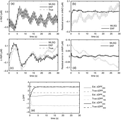
EKF and WLSQ solutions for simulated NIRS data: (a) calculated using EKF and WLSQ and the true known sequence; (b) residual errors in for EKF and WLSQ; (c) calculated using EKF and WLSQ; (d) residual errors for ; (e) terms calculated using EKF. The true errors are shown in dotted lines.
In the simulated data, we had explicit prior knowledge of the measurement noise variance based on the simulated WGN that was introduced in . The process noise variances and were found to be approximately . Results from tuning the process noise variance in are shown in Fig. 2. A minimum value in the percent mean RSS error occurs at . This value of was used in the EKF applied to both the simulated and experimental NIRS data.
Fig. 2.

Percent mean RSS error between known and and the solutions computed using EKF for nine evaluated levels of . The minimum RSS error corresponds to a process noise variance of .
Figure 3(a) shows the percent cross-talk error in the solutions obtained from EKF and WLSQ. The percent cross-talk error in is significantly smaller in EKF relative to that found for WLSQ across all frequency bands (paired -test, ). Although the cross-talk error in is slightly higher for EKF in the HF and CARDIAC band, the corresponding values in WLSQ are much higher at 45.9% and 35.1%, respectively.
Fig. 3.
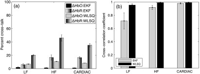
Simulated NIRS data residual analysis: (a) percent cross-talk error in and solution obtained using EKF ad WLSQ. Error bars show standard error; (b) mean sum squared cross-correlation coefficients for LF, HF, and CARDIAC filtered residuals for EKF and WLSQ.
Figure 3(b) shows the mean of the sum squared cross correlation coefficients obtained for the LF, HF, and CARDIAC frequency bands for EKF and WLSQ applied to simulated NIRS data. We can observe that the EKF has reduced mean sum squared cross-correlation coefficient values in the LF band relative to WLSQ. In case of the HF and CARDIAC bands, the mean squared cross-correlation coefficient values for EKF and WLSQ are comparable.
The results from EKF and WLSQ applied to experimental NIRS data segments are shown in Fig. 4. and computed using EKF agree closely with the WLSQ results [Fig. 4(a) and 4(b)]. Figure 4(c) shows the values calculated for wavelengths of 690, 785, and 830 nm. Large deviations in the values occur between 125 and 140 s. During this time interval, the difference between the EKF and WLSQ solution for and is also large [Fig. 4(d)]. The values for the plotted time interval are 0.97 for and 0.98 for .
Fig. 4.
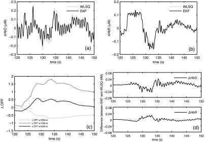
EKF and WLSQ results obtained for experimental NIRS data collected from subject 3 (a) estimated using WLSQ and EKF (b) corresponding estimated using WLSQ and EKF; (c) EKF estimates of at 690, 785, and 830 nm; (d) difference between WLSQ and EKF hemodynamic signals.
Figure 5 shows and results in the LF, HF and CARDIAC bands for EKF and WLSQ. The differences between the EKF and WLSQ solutions are also plotted.
Fig. 5.
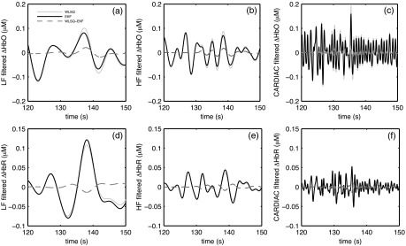
Band pass filtered (upper row) and (lower row) sequences from EKF and WLSQ for subject 3: (a) and (d) LF (0.04 to 0.15 Hz); (b) and (e) HF (0.15 to 0.4 Hz); (c) and (f) CARDIAC (0.4 to 2.0 Hz).
Figure 6 shows the residuals obtained for WLSQ and EKF and their autocorrelation sequences for subject 3. The WLSQ and EKF residuals shown in Fig. 6(a) and 6(b) appears to contain physiological signal components such as cardiac oscillations in the EKF residuals. There also appear to be low frequency components in both the WLSQ and EKF residuals. The autocorrelation structures shown in Fig. 6(c) and 6(d) shows reduced serial correlation at larger lags in EKF compared to WLSQ. The autocorrelation values for the 690 nm residual appear to be substantially smaller in EKF compared to WLSQ.
Fig. 6.
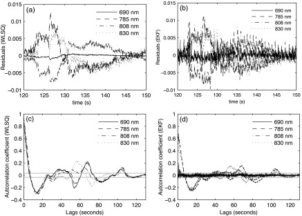
(a) WLSQ residuals for wavelengths 690, 758, 808, and 830 nm; (b) EKF residuals for the four wavelengths; (c) autocorrelation coefficients for residuals from WLSQ with the 95% confidence interval shown in solid gray lines (d) autocorrelation coefficient of residuals from EKF with the 95% confidence interval shown in solid gray lines.
Table 1 summarizes the mean percentages of points in the autocorrelation functions for WLSQ and EKF that fall outside of the 95% confidence intervals. The percentages of points outside the confidence bounds for EKF are consistently smaller than for WLSQ.
Table 1.
Mean percentages of points that fall outside of the 95% confidence intervals for the EKF and WLSQ autocorrelation functions.
| Wavelength (nm) | WLSQ (%) | EKF (%) |
|---|---|---|
| 690 | 39.6 | 4.1 |
| 785 | 41.9 | 34.4 |
| 808 | 41.1 | 29.2 |
| 830 | 38.4 | 21.7 |
Figure 7 compares the mean squared cross-correlation coefficient values obtained in the analysis of EKF and WLSQ residuals. All three subjects have smaller mean squared correlation coefficient values for EKF relative to those found for WLSQ (see Table 2 for ANOVA). The lowest mean squared cross-correlation coefficients were found for the HF band in EKF.
Fig. 7.

Mean squared cross-correlation coefficients of residuals from the analysis of experimental data from three subjects. Results are shown for LF, HF and CARDIAC frequency bands with standard error bars.
Table 2.
NOVA of mean squared cross-correlation values shown in Fig. 7.
| Factor | Sum Sq. | d.f. | Mean Sq. | F | P-value |
|---|---|---|---|---|---|
| LF (0.04–0.15 Hz) | |||||
| Wavelength | 6.060 | 5 | 1.212 | 7.39 | |
| Subject | 0.027 | 2 | 0.013 | 0.08 | 0.9217 |
| Algorithm | 2.400 | 1 | 2.400 | 14.63 | |
| Error | 10.34 | 63 | 0.164 | ||
| Total | 18.82 | 71 | |||
| LF (0.04–0.15 Hz) | |||||
| Wavelength | 6.499 | 5 | 1.299 | 10.90 | |
| Subject | 0.269 | 2 | 0.134 | 1.13 | 0.3289 |
| Algorithm | 1.415 | 1 | 1.415 | 11.87 | |
| Error | 7.512 | 63 | 0.119 | ||
| Total | 15.697 | 71 | |||
| CARDIAC (0.4–2.0 Hz) | |||||
| Wavelength | 5.329 | 5 | 1.065 | 12.83 | |
| Subject | 0.002 | 2 | 0.001 | 0.01 | 0.9863 |
| Algorithm | 2.699 | 1 | 2.699 | 32.49 | |
| Error | 5.234 | 63 | 0.083 | ||
| Total | 13.27 | 71 | |||
ANOVA results are summarized in the Table 2. Algorithm (EKF versus WLSQ) contributes significantly () in all three frequency bands. Therefore, we can reject the null hypothesis that the mean squared cross-correlation coefficient values found for EKF and WLSQ are the same at those frequency bands. It is interesting to note that the wavelength factor also contributes significantly to the variability in the mean squared cross-correlation coefficient values indicating that the EKF corrections vary significantly with wavelength.
Figure 8 shows the mean percent deviations between EKF and WLSQ solutions in the LF, HF and CARDIAC frequency bands. For each frequency band, the mean percent deviations in and are significantly different from zero (two-tailed -test: ). The mean deviation over all frequency bands was found to be 4.04% for and 4.92% for . In the LF band, the mean percent deviations are comparable for both and . The mean percent signal deviation is smaller in compared to in the HF and CARDIAC bands ().
Fig. 8.

Mean percent deviations between EKF and WLSQ solutions filtered in the LF, HF, and CARDIAC frequency bands shown with 95% confidence intervals from a paired -test.
6. Discussion and Conclusion
The proposed EKF algorithm is able to calculate and from simulated NIRS data by continuously updating values. We observed in simulation that the residual errors in and decrease rapidly within the first 2 s as the EKF tracked the errors introduced in . In the analysis of experimental data, we observed reduced autocorrelation of residuals for EKF compared to WLSQ. We believe that the superior performance of EKF is achieved due to weighting of the state variable innovations by the optimal Kalman gain at each time step. The application of the Kalman gain in this way helps to minimize the posterior error covariance over time. In WLSQ, the measurement data is weighted by constant factors over all time steps; so even though the solution is optimal in the least squares sense, WLSQ lacks the flexibility of EKF to account for time variation in . As a result, EKF outperforms WLSQ in the estimation of and .
We observed reduced cross-correlations in the residuals in wavelength pairs for EKF in the LF, HF and CARDIAC bands compared to WLSQ, which is consistent with the reduction of cross-talk error. Convergence of the EKF state estimates to the true states is dependent on prior knowledge of the process noise and measurement noise variance statistics. In the proposed method, we demonstrate how to obtain prior estimates of those statistics based on minimizing the residual error in EKF.
We also quantified the differences in the hemodynamic signals calculated using EKF and WLSQ in physiologically relevant frequency bands. We found significant differences in the sequences in the LF and HF bands. The average of differences between EKF and WLSQ solutions across all frequency bands was 3.75% for and 4.57% for . We believe that this difference is due to a reduction of cross-talk error in and obtained using EKF. This is supported by the observation that the EKF solution obtained from simulated NIRS data had reduced cross-talk error relative to the WLSQ solutions. In the simulation, the errors in and from the known sequences were significantly lower in the EKF results compared to the WLSQ results.
The proposed EKF method offers several advantages over other methods that may be used to calculate . Unlike other studies where is estimated based on the assumption that it is constant over time,2,25,31 the proposed EKF algorithm continuously updates and it can account for variation in due to differences in anatomical structure and tissue composition of the brain. In cases where relative calibration of and is desired, the proposed method eliminates the need to measure using TD or FD instruments or applying simulation techniques discussed in Sec. 2.
The proposed EKF algorithm has potential applications in the clinical investigation of brain injury. A number of recent studies have used NIRS to monitor patients during stroke rehabilitation and recovery.32–34 A limitation in these studies is the inability to accurately quantify cerebral hemodynamics in a region of interest. In the above referenced stroke studies, is assumed to be constant over time and the studies did not account for possible variation due to the stroke. However, could deviate substantially in stroke because of the high absorption coefficient of hemoglobin. As a result, the calculated and may not have accurately reflected the hemodynamics in those patients. The proposed algorithm could also be applied to other clinical diagnostic applications of NIRS such as breast cancer detection.35 The optical properties of cancerous tissue are different from those of healthy tissue in the breast. Accurate assessment of hemodynamic changes in breast tissue also relies on using accurate estimates of DPF in the NIRS spectroscopic calculations. Further investigation is required to determine if the proposed EKF algorithm is able to correct path length errors in NIRS applications in stroke, cancer, and other clinical conditions.
References
- 1.Delpy D. T., Cope M., “Quantification in tissue near-infrared spectroscopy,” Phil. Trans. R. Soc. Lond. B 352(1354), 649–659 (1997). 10.1098/rstb.1997.0046 [DOI] [Google Scholar]
- 2.Duncan A., et al. , “Optical pathlength measurements on adult head, calf and forearm and the head of the newborn infant using phase resolved optical spectroscopy,” Phys. Med. Biol. 40(2), 295–304 (1995). 10.1088/0031-9155/40/2/007 [DOI] [PubMed] [Google Scholar]
- 3.Delpy D. T., et al. , “Estimation of optical pathlength through tissue from direct time of flight measurement,” Phys. Med. Biol. 33(12), 1433–1442 (1988). 10.1088/0031-9155/33/12/008 [DOI] [PubMed] [Google Scholar]
- 4.Selb J., Joseph D. K., Boas D. A., “Time-gated optical system for depth-resolved functional brain imaging,” J. Biomed. Opt. 11(4), 044008 (2006). 10.1117/1.2337320 [DOI] [PubMed] [Google Scholar]
- 5.White B. R., Culver J. P., “Quantitative evaluation of high-density diffuse optical tomography: in vivo resolution and mapping performance,” J. Biomed. Opt. 15(2), 026006 (2010). 10.1117/1.3368999 [DOI] [PMC free article] [PubMed] [Google Scholar]
- 6.Franceschini M. A., et al. , “Diffuse optical imaging of the whole head,” J. Biomed. Opt. 11(5), 054007 (2006). 10.1117/1.2363365 [DOI] [PMC free article] [PubMed] [Google Scholar]
- 7.Cope M., et al. , “Methods of quantitating cerebral near infrared spectroscopy data,” Adv. Exp. Med. Biol. 222, 183–189 (1988). [DOI] [PubMed] [Google Scholar]
- 8.Ultman J. S., Piantadosi C. A., “Differential pathlength factor for diffuse photon scattering through tissue by a pulse-response method,” Math. Biosci. 107(1), 73–82 (1991). 10.1016/0025-5564(91)90072-Q [DOI] [PubMed] [Google Scholar]
- 9.Bonnéry C., et al. , “Changes in diffusion path length with old age in diffuse optical tomography,” J. Biomed. Opt. 17(5), 056002 (2012). 10.1117/1.JBO.17.5.056002 [DOI] [PubMed] [Google Scholar]
- 10.Strangman G., Franceschini M. A., Boas D. A., “Factors affecting the accuracy of near-infrared spectroscopy concentration calculations for focal changes in oxygenation parameters,” NeuroImage 18(4), 865–879 (2003). 10.1016/S1053-8119(03)00021-1 [DOI] [PubMed] [Google Scholar]
- 11.Yoshitani K., et al. , “Effects of hemoglobin concentration, skull thickness, and the area of the cerebrospinal fluid layer on near-infrared spectroscopy measurements,” Anesthesiology 106(3) 458–462 (2007). 10.1097/00000542-200703000-00009 [DOI] [PubMed] [Google Scholar]
- 12.Okada E., Delpy D. T., “Near-infrared light propagation in an adult head model. I. Modeling of low-level scattering in the cerebrospinal fluid layer,” Appl. Opt. 42(16), 2906–2914 (2003). 10.1364/AO.42.002906 [DOI] [PubMed] [Google Scholar]
- 13.Benaron D. A., Kurth C. D., Steven J. M., “Transcranial optical path length in infants by near-infrared phase-shift spectroscopy,” J. Clin. Monit. 11(2), 109–117 (1995). 10.1007/BF01617732 [DOI] [PubMed] [Google Scholar]
- 14.Yoshitani K., et al. , “Measurements of optical pathlength using phase-resolved spectroscopy in patients undergoing cardiopulmonary bypass,” Anesth. Analg. 104 (2), 341–346 (2007). 10.1213/01.ane.0000253508.97551.2e [DOI] [PubMed] [Google Scholar]
- 15.Muehlschlegel S., et al. , “Feasibility of NIRS in the neurointensive care unit: a pilot study in stroke using physiological oscillations,” Neurocrit. Care 11(2) 288–295 (2009). 10.1007/s12028-009-9254-4 [DOI] [PMC free article] [PubMed] [Google Scholar]
- 16.Kim M. N., et al. , “Noninvasive measurement of cerebral blood flow and blood oxygenation using near-infrared and diffuse correlation spectroscopies in critically brain-injured adults,” Neurocrit. Care 12(2), 173–180 (2010). 10.1007/s12028-009-9305-x [DOI] [PMC free article] [PubMed] [Google Scholar]
- 17.Oki Y., Kawaguchi H., Okada E., “Validation of practical diffusion approximation for virtual near infrared spectroscopy using a digital head phantom,” Opt. Rev. 16(2), 153–159 (2009). 10.1007/s10043-009-0026-3 [DOI] [Google Scholar]
- 18.Gao F., Niu H., Zhao H., “The forward and inverse models in time-resolved optical tomography imaging and their finite-element method solutions,” Image Vis. Comput. 16(9), 703–712 (1998). 10.1016/S0262-8856(98)00078-X [DOI] [Google Scholar]
- 19.Arridge S. R., Cope M., Delpy D. T., “The theoretical basis for the determination of optical pathlengths in tissue: temporal and frequency analysis,” Phys. Med. Biol. 37(7), 1531–1560 (1992). 10.1088/0031-9155/37/7/005 [DOI] [PubMed] [Google Scholar]
- 20.Fukui Y., Ajichi Y., Okada E., “Monte Carlo prediction of near-infrared light propagation in realistic adult and neonatal head models,” Appl. Opt. 42(16), 2881–2887 (2003). 10.1364/AO.42.002881 [DOI] [PubMed] [Google Scholar]
- 21.Okada E., et al. , “Theoretical and experimental investigation of near-infrared light propagation in a model of the adult head,” Appl. Opt. 36(1), 21–31 (1997). 10.1364/AO.36.000021 [DOI] [PubMed] [Google Scholar]
- 22.Uludag K., et al. , “Cross talk in the Lambert-Beer calculation for near-infrared wavelengths estimated by Monte Carlo simulations,” J. Biomed. Opt. 7(1), 51–59 (2002). 10.1117/1.1427048 [DOI] [PubMed] [Google Scholar]
- 23.Hiraoka M., et al. , “A Monte Carlo investigation of optical pathlength in inhomogeneous tissue and its application to near-infrared spectroscopy,” Phys. Med. Biol. 38(12), 1859–1876 (1993). 10.1088/0031-9155/38/12/011 [DOI] [PubMed] [Google Scholar]
- 24.Okui N., Okada E., “Wavelength dependence of crosstalk in dual-wavelength measurement of oxy- and deoxy-hemoglobin,” J. Biomed. Opt. 10(1), 011015 (2005). 10.1117/1.1846076 [DOI] [PubMed] [Google Scholar]
- 25.Zhao H., et al. , “Maps of optical differential pathlength factor of human adult forehead, somatosensory motor and occipital regions at multi-wavelengths in NIR,” Phys. Med. Biol. 47(12), 2075–2093 (2002). 10.1088/0031-9155/47/12/306 [DOI] [PubMed] [Google Scholar]
- 26.Huppert T. J., et al. , “HomER: a review of time-series analysis methods for near-infrared spectroscopy of the brain,” Appl. Opt. 48(10), D280–D298 (2009). 10.1364/AO.48.00D280 [DOI] [PMC free article] [PubMed] [Google Scholar]
- 27.Robertson F. C., Douglas T. S., Meintjes E. M., “Motion artifact removal for functional near infrared spectroscopy: a comparison of methods,” IEEE Trans. Biomed. Eng. 57 (6), 1377–1387 (2010). 10.1109/TBME.2009.2038667 [DOI] [PubMed] [Google Scholar]
- 28.Holman J. P., Experimental Methods for Engineers, 4th ed., McGraw-Hill Inc., New York: (1984). [Google Scholar]
- 29.Camm A., et al. , “Heart rate variability-Standards of measurement, physiological interpretation, and clinical use,” Circulation 93(5), 1043–1065 (1996). 10.1161/01.CIR.93.5.1043 [DOI] [PubMed] [Google Scholar]
- 30.Fisher R. A., “On the ‘probable error’ of a coefficient of correlation deduced from a small sample,” Metron 1(4), 3–32 (1921). [Google Scholar]
- 31.Umeyama S., “New method of estimating wavelength-dependent optical path length ratios for oxy-and deoxyhemoglobin measurement using near-infrared spectroscopy,” J. Biomed. Opt. 14(5), 054038 (2009). 10.1117/1.3253350 [DOI] [PubMed] [Google Scholar]
- 32.Strangman G., et al. , “Near-infrared spectroscopy and imaging for investigating stroke rehabilitation: test-retest reliability and review of the literature,” Arch. Phys. Med. Rehabil. 87(12), 12–19 (2006). 10.1016/j.apmr.2006.07.269 [DOI] [PubMed] [Google Scholar]
- 33.Eliassen J. C., et al. , “Brain-mapping techniques for evaluating poststroke recovery and rehabilitation: a review,” Top. Stroke Rehabil. 15(5), 427–450 (2008). 10.1310/tsr1505-427 [DOI] [PMC free article] [PubMed] [Google Scholar]
- 34.Lin P. Y., et al. , “Review: applications of near infrared spectroscopy and imaging for motor rehabilitation in stroke patients,” J. Med. Biol. Eng. 29(5), 210–221 (2009). [Google Scholar]
- 35.Fantini S., Sassaroli A., “Near-infrared optical mammography for breast cancer detection with intrinsic contrast,” Ann. Biomed. Eng. 40(2), 398–407 (2012). 10.1007/s10439-011-0404-4 [DOI] [PMC free article] [PubMed] [Google Scholar]