Mapping and Cracking Sensorimotor Circuits in Genetic Model Organisms

Abstract

One central goal of systems neuroscience is to understand how neural circuits implement the computations that link sensory inputs to behavior. Work combining electrophysiological and imaging-based approaches to measure neural activity with pharmacological and electrophysiological manipulations has provided fundamental insights. More recently, genetic approaches have been used to monitor and manipulate neural activity, opening up new experimental opportunities and challenges. Here, we discuss issues associated with applying genetic approaches to circuit dissection in sensorimotor transformations, outlining important considerations for experimental design and considering how modeling can complement experimental approaches.

Introduction

A primary goal of neuroscience is to understand how the brain computes. Over more than 100 years, detailed studies of sensory systems and motor outputs have related neural activity to stimuli and responses and provided a rich, quantitative framework for understanding a fundamental neural computation, the transformation of sensory input into behavioral output. However, establishing causal links between sensory inputs, circuit activity, and behavioral outputs has proven challenging. The recent development of tools for manipulating and monitoring neural activity in genetic model organisms (reviewed in (Fenno et al., 2011; Luo et al., 2008; Venken et al., 2011)) has enabled a marriage of genetics and systems neuroscience. These tools can define types of neurons, establishing neuronal identity independent of activity pattern or morphology. In addition, a wealth of genetic effectors allows neural activity to be measured and manipulated in cell-type specific ways. These tools reveal correlations between activity and behavior, and more importantly, help establish causal relationships between neurons, circuits, and behaviors. Finally, model organisms have relatively compact brains, with reasonably stereotyped complements of cell types and connections. Together, these advantages promise high-resolution dissection of neural circuit function. In this Perspective, we highlight central questions to consider when measuring, modulating, and modeling neural activity in sensorimotor circuits.

In its basic form, neural circuit dissection seeks to establish specific relationships between a Stimulus X, Behavior Y and activity in Neuron Z. One simple (and likely unrealistic) hypothesis is that each of these entities is one-dimensional such that stimulus X either activates or inhibits neuron Z and promotes or inhibits behavior Y. With this assumption, the predicted effects of genetically manipulating the activity of neuron Z are limited to promoting or inhibiting a behavior, and neuron Z’s function is described as ‘necessary’ or ‘sufficient’, terms taken from the lexicon of genetics. With this approach, it is possible to define some basic circuit components by “breaking” the circuit and monitoring the behavioral outcome. It is critical to keep in mind that these assignments are not themselves descriptions of how the circuit computes, but they are useful constraints on circuit models. These constraints have three components. First, one can construct a catalog of stimuli and behaviors affected by the activity of specific types of neurons and thus identify the relevance of these discrete populations of neurons within circuits. Second, if the behavior being examined exhibits an increase or decrease in magnitude, it is possible to determine whether the neuron promotes or inhibits the behavior. Finally, by simultaneously manipulating neurons at multiple stages in a circuit, it is possible to perform a circuit equivalent of genetic epistasis to order different neuron types into hierarchical pathways within a network. Ongoing efforts in many systems are establishing such pathway constraints and have greatly increased our basic understanding of neuronal circuitry. However, the core weakness of this approach is that sensory inputs and behavioral outputs are multidimensional and any neural manipulation or stimulus modification likely affects behavior differently along different dimensions. Furthermore, it is unlikely that the function of any neuron is to simply modulate the strength of the coupling between a stimulus and a response. Thus, the conclusions drawn from ‘circuit breaking’ experiments are shaped, and potentially biased, not only by the structure and function of the neural circuits involved, but also by the stimuli used and how neural activity and behavior are measured and represented. Accordingly, it is critical to incorporate the breadth of potential stimuli and behavioral responses into experiments that use genetic tools to manipulate neural activity. These experiments can be more difficult, but this deeper understanding will capture how the elaborate architecture of the brain and the biophysical properties of neural networks give rise to the dynamic, evolving character of behavior and its modulation by the dynamic sensory experience. Overall, it is critical to understand how one’s a priori assumptions regarding the dimensionality of the variables within a circuit influences experimental design and interpretation of genetic circuit breaking experiments. While many of the considerations discussed herein would hold true for examining circuitry in general, we will use sensorimotor circuits as a platform to highlight points to consider when using genetic model systems to dissect neuronal circuits.

How are the bounds of a circuit defined?

At the outset, the experimenter should aim to define an operational bound on the circuit components of interest. In sensorimotor behaviors, such a circuit clearly includes the connected set of neurons that start with sensation and end with the motor output. However, this is an overly simplified description, since these circuits are often influenced both by additional sensory modalities and by top-down inputs from other brain regions. Thus, we should consider two types of inputs into sensorimotor circuits: proximal inputs from the environment and modulatory (or gating) inputs from other brain regions that represent the animal’s goals and state. To limit complexity when exploring circuit function, one could consider only those neurons whose activities change on timescales comparable to the stimuli and behaviors under investigation. For example, the analysis could be restricted to circuit components that are directly involved in the immediate sensorimotor transformation. Alternatively, one could assess the circuit components that modulate the transformation on fast timescales, effectively changing the computation of the network, thereby including sensory cues that act only indirectly on motor outputs (e.g. pheromones that affect arousal) and phenomena like selective attention, which can rapidly reshape a sensorimotor transformation. Thus, selecting circuitry based on time scale would separate circuit components that control a fast sensorimotor transformation from those that control, for instance, a circadian rhythm that modulates it. From a practical standpoint, then, a core goal is to hold the activities of these slowly varying circuit elements stationary across each experiment.

Within this broad bound, it is often possible and useful to identify subcircuit modules that perform particular steps in a sensorimotor transformation. For example, one module might be involved in identifying an odor, while another is involved in generating the appropriate behavioral response. Modules may be arranged sequentially so that the output of one acts as an input to a downstream module. Alternatively, they may be arranged in parallel, allowing for both divergent and convergent processing. Analogously, computations can be segmented into discrete elements or “building blocks” that can be used in multiple, distinct sensorimotor circuits, so that studying computational modules in one context can provide insight into similar operations in other circuits.

How are sensory inputs defined?

To dissect sensorimotor circuit function, one must establish the realm of sensory inputs. For any sensory system, the physical properties of the detector define the limits of sensory inputs. For example, individual photoreceptors are tuned to particular wavelength ranges, have limited dynamic range, exhibit spatial and temporal filtering, and perform significant adaptation (Arshavsky and Burns, 2012; Baylor and Fuortes, 1970; Baylor and Hodgkin, 1974; Baylor et al., 1974; Stavenga, 2002; Wald, 1949). As information that is not captured by peripheral sensors cannot be recovered by downstream circuit operations, how the sensor reshapes and represents the input signal strictly limits what the brain knows about the world.

Sensory inputs are typically high-dimensional. In the case of vision, for example, a full description of the stimulus would include the spectral composition and photon count across all of visual space as a function of time. However, natural stimuli are highly structured, with many particular combinations of stimulus features being over-represented. For instance, for most animals, many visual objects are large enough that they are simultaneously detected by more than one photoreceptor. Similarly, individual odorant concentrations can be correlated or anti-correlated with each other, creating odor combinations that represent specific environments or objects. An animal may also influence the statistics of its environment, either by inhabiting a certain environment or by moving in a way that creates particular spatial or temporal sampling patterns. For example, by generating a particular velocity distribution, motor outputs can shape the pattern of visual inputs (Egelhaaf et al., 2012; Kern et al., 2001; O’Carroll et al., 1996). Similarly, in rodents, breathing alters the temporal pattern of olfactory cues, while the pattern of whisker movements shapes somatosensation (Carvell and Simons, 1990; Smear et al., 2011). Finally, in social behaviors, sensory cues are provided in a temporal pattern that depends on the movements and actions of multiple animals, as well as on their interactions, further increasing stimulus dimensionality. Fortunately, many social behaviors, including mating or aggression can also display significant stereotypy (Hall, 1994; Liu and Sternberg, 1995; Stone, 1922), creating a measure of predictability that the brain can exploit.

In this context, one can think of the processing in downstream sensory circuits as extracting relevant low dimensional features, such as visual motion or odor identity, from very high dimensional input spaces. Naturally occurring or behaviorally-induced statistical correlations in the inputs can then be exploited by the circuit to extract sensory information efficiently. This can be done in a ‘lossy’ manner, where features of interest are captured and other information is discarded (Barlow, 1953; Lettvin et al., 1959). Alternately, it can be done in a ‘lossless’ manner, where redundancy in the signal is removed and some features are highlighted without losing the ability to reconstruct the original signal (Atick, 1992; Barlow, 1961; Field, 1994; Hateren, 1992; Olshausen and Field, 1996). Ultimately, behavioral responses are intrinsically lossy computations, as they reduce the sensory stimulus to a single, selected response. As a result, it seems unlikely that any sensory system implements truly lossless encoding. Rather, in every sensory system, selective filtering likely begins very early on in the processing stream.

How can sensory stimuli be chosen experimentally?

Given the breadth of the sensory environment it is rare that any experiment could probe all possible inputs. As a result, determining the subset of inputs to explore represents a critical experimental decision. One’s intuition about biology, particularly the ethological context of the behavior, obviously plays an important role in the choice of a stimulus. Indeed, in the case of social behaviors, the choice of an appropriate stimulus is likely significantly constrained by the context necessary to evoke the behavior at all. However, for many sensorimotor circuits other strategies for selecting stimuli are also worth considering. A long tradition in neuroscience has involved the use of relatively simple stimuli that represent some fundamental aspect of a sensory cue. For example, to examine visual motion detection, square wave gratings that comprise alternating contrast stripes have long been used to elicit motion responses (Andermann et al., 2011; Brockerhoff et al., 1995; Campbell et al., 1969; Götz, 1964; Götz and Wenking, 1973; Hecht and Wald, 1934; Marshel et al., 2011; Niell and Stryker, 2008; Orger et al., 2000; Prusky et al., 2000). These have provided powerful insights, identifying motion-sensitive neurons and circuits in flies, fish, and mice and building upon previous work describing direction selective neurons in other model animals (Barlow and Hill, 1963; Kozak et al., 1965; Maunsell and Van Essen, 1983). Yet even these simple stimuli are complex in their neural processing. For example, when square wave gratings were used to distinguish the functions of two early visual processing pathways in Drosophila, few differences were seen (Rister et al., 2007). It was only when even simpler stimuli, consisting of single bright or dark edges, were used that stark functional differences between the pathways were observed (Clark et al., 2011; Joesch et al., 2010). Simplicity is thus in the eye of the beholder – or rather in the response of the circuitry.

In guiding the selection of simple stimuli, there is often an informative minimum set of inputs required for a given computation. For example, to perceive motion requires at least two spatially separated sensors that are stimulated by changes in light intensity at two points in time (Poggio and Reichardt, 1973). More broadly, limiting the extent of stimulus presentation (whether in duration, space or any other stimulus parameter) allows one to describe the minimal amount of sensory information needed to evoke the behavior of interest. This approach affords two important advantages. First, limiting the stimulus presentation reduces the exposure of these circuits to the cues that drive adaptation, allowing better control of adaptation state across an experiment. Second, when a circuit’s response is barely evoked, it is sensitized to modulation, making it more likely that that targeted genetic manipulations of small groups of neurons will produce changes in the response.

Without knowing what the minimal input might be, the principled approach of linear systems analysis postulates a specific input-output structure that can be measured experimentally. With linear systems analysis one can relate any number of dynamically changing stimulus characteristics to behavioral or neural responses using particular types of inputs (see Figure 1). In this context, the simple operational definition of a linear system is that its response to a weighted sum of inputs equals the weighted sum of the responses to each input individually. Importantly, it is often possible to determine whether a system is linear by testing whether this input-output relationship holds. Furthermore, even highly non-linear systems generally respond linearly to small variations in stimulus strength (Marmarelis, 2004) (with some notable exceptions (Eguiluz et al., 2000)). As a result, brief or low amplitude stimulus presentations can provide regimes where this analysis is applicable to many complex circuits. For example, the temporal response properties of visual neurons to contrast can be described using stimuli that vary in intensity, increasing or decreasing in brightness either stably (forming a “step”) or transiently (making an “impulse”), or from continuously varying noise (Figures 1A and 1B) (Baylor et al., 1974; McCann, 1974). From these stimuli, one can derive mathematical functions, or filters, to describe the system’s response as a weighted average of its previous inputs. For any temporal pattern of input signals within the linear range, this filter can be used to describe the dynamics of the system’s output. Often, a static non-linearity is applied to the output of the linear filter in order to account for saturation or rectification effects, forming what is called a linear non-linear (LN) model (Figure 1C) (Baccus and Meister, 2002; Chichilnisky, 2001; Sakai et al., 1988). Linear filters can predict responses to any input as long as the model assumptions hold, and can describe neural responses recorded using either electrophysiological approaches (Baccus and Meister, 2002; Kim and Rieke, 2001) or calcium imaging (Clark et al., 2011; Ramdya et al., 2006), as well as behavioral responses (Aptekar et al., 2012; Clark et al., 2011; Rohrseitz and Fry, 2011; Theobald et al., 2010). However, in some cases, these methods produce poor fits to observed responses, indicating that the underlying assumptions are violated. A single LN system, for instance, may not capture the behavior of a circuit across a wide range of inputs (see, for instance, (Daly and Normann, 1985)). Similarly, this model cannot be used when the gain of a system is itself a function of its inputs (Olsen et al., 2010). In addition, adapting systems often require multiple fits to the LN model (Baccus and Meister, 2002). In sum, these approaches can capture a system’s properties under some regimes, but tend to underestimate the extent of the non-linear operations that circuits perform, many of which may be crucial to how the circuit functions in the presence of natural stimuli.

Figure 1.

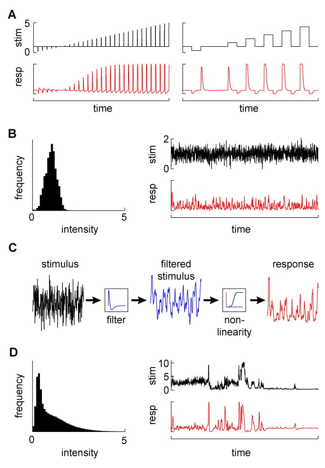
Probing a system with different stimuli. (A) Examples of pulse and step changes in stimuli (top) and simulated responses (bottom). (B) A Gaussian stimulus. The left plot shows the distribution of Gaussian stimulus values (with mean 1), while the right plots show a Gaussian noise stimulus (top) and a simulated sample response (bottom). (C) Explanation of the LN model. In the model, stimuli (left trace) are first passed over with a linear filter to produce a weighted average of the stimulus (middle trace). That filtered stimulus is mapped onto the response (right trace) with a function that may contain non-linearities. The filter can be estimated from the system response to a Gaussian noise input, after which the mapping function can be fit to the data. The function is linear in the case of the linear system, or can account for post-filtering non-linearities that occur quickly compared to the filtering process, for instance to prevent very strong responses (create saturation) or to prevent negative responses (create rectification). (D) A natural stimulus (from (Van Hateren, 1997)). In the distribution on the left, note the infrequent but large stimulus values (the mean is set to 1). A natural time series of that distribution, incorporating naturalistic dynamics (top), along with a simulated sample response to that stimulus (bottom).

Approaches that focus on using the simplest of stimuli neglect the complexity of the sensory environment that neural systems have evolved to process. Natural stimuli are often not near perceptual thresholds, can contain large variations in stimulus amplitude, and are highly structured (Figure 1D) (Ruderman and Bialek, 1994; Van Hateren, 1997). In addition, natural stimuli often stimulate multiple sensory systems, requiring the brain to integrate information across modes. Such naturalistic stimuli can be used to probe sensory systems in more challenging regimes, but when the evoked responses are not predicted by impulse or step responses, or by a model, it becomes difficult to tease out which aspects of the ethologically-relevant stimulus resulted in the observed behavior (Boeddeker et al., 2005; David et al., 2004; Rajan and Bialek, 2012). Yet, the functional characteristics of a circuit that defy extrapolation from simple to natural stimuli are perhaps the most interesting and may constitute mechanisms that enhance or suppress specific aspects of sensory information. Thus, comparing responses to simple, artificial stimuli to those evoked by natural stimuli would point towards what information the system is built to extract. In truth, although the requirement to compare natural and simple artificial stimuli responses is widely recognized in the field, direct comparisons are rare because it is not trivial to parse a natural stimulus into simpler stimuli that optimally stimulate a circuit. Consider vision for instance: should we probe circuits with lines (Hubel and Wiesel, 1962), edges (Schiller et al., 1976), Gabor filters (Daugman, 1985), random dot patterns (Baker et al., 1981), textural correlations (Julész et al., 1978), or rather attempt to extract those natural features most relevant to the system (Rajan and Bialek, 2012)? Each of these approaches has value, and the answer on how to proceed will not be universal, but rather circuit dependent. It is important to note that some natural sensory cues are so specific that no reasonable decomposition is possible. For example, pheromonal cues that guide social behaviors can be exquisitely unique to the organism and presented only under specific circumstances (Bray and Amrein, 2003; Kimchi et al., 2007). Nonetheless, during many social interactions multiple sensory cues are presented in conjunction and can play a role in modulating the behavior. In this context, reducing the complex mixture of cues to individual components can reveal how specific behavioral components are linked to single natural sensory cues.

While a linear model makes a single prediction for the response of a system, there are an infinite number of ways for a system to be non-linear. One approach, then, is to simply “guess and test” by hypothesizing what forms of non-linearities likely characterize it. For example, a response shaped by inhibition as well as excitation may linearly depend on its inputs if they are simply added together, but be non-linear if they are multiplied or divided (Olsen et al., 2010; Silver, 2010). Provided with a set of hypotheses, one could then probe the circuit with inputs that would distinguish between them and additional stimuli can then be designed to fit the parameters of the model. While analytical methods for dissecting non-linearities are not as canonized as linear systems analysis, a number of important methods (for example Volterra series expansions, bispectral analysis, and non-linear dynamic systems analysis) have all been applied to neural and behavioral signals in a variety of experimental settings to reveal how different stimuli give rise to different circuit outputs (Bullock et al., 1997; Marmarelis, 2004; Poggio and Reichardt, 1980; Sigl and Chamoun, 1994; Stephens et al., 2008). Further development and application of approaches to non-linear systems analysis are likely to be critical to studies of behavioral responses elicited by complex, ethologically relevant stimuli.

In order to probe neural circuits with naturalistic stimuli, it is also useful to consider how ethological multisensory inputs might shape circuit computation. Three questions emerge. First, to what extent are the interactions between different sensory inputs tightly tuned for particular stimuli? At one extreme, very specific combinations of sensory inputs may be needed to elicit a unique behavioral response, as in the case of male aggression in mice (Stowers et al., 2002). Alternatively, the presence of a cue from one sensory modality could simply alter the gain of the response to other cues, as is seen with the presence of an attractive odor in a visually-guided odor localization strategy (Duistermars and Frye, 2008; Frye et al., 2003). Second, at what level in the processing pathway does integration occur? For example, the null hypothesis for multisensory integration would be that different types of sensory inputs are processed independently, and then combined only in motor centers, during the shaping of the behavioral response. Alternatively, integration could occur early in sensory processing pathways, reshaping the perception of one sensory input as a function of the characteristics of another (Cohen et al., 2011). Finally, what operation does the brain perform to integrate the cues in question? For example, if integration occurs at the level of behavior, it can be a simple summation of the individual behavioral responses to each cue (Frye and Dickinson, 2004). More interestingly, the response to one cue can be gated by the characteristics of the other, such that the presence of one stimulus determines how the animal responds to the second input (Chow et al., 2011). The first of these modes of cue integration could be treated as linear, while the second clearly reflects non-linear combination and exemplify how naturalistic stimuli affect the choice of experimental and analytical strategies.

How are behavioral outputs defined?

Since behavior is the ultimate output of a circuit, it provides a powerful tool to assess the contribution of individual neurons to circuit function. At one level, the simple fact that a sensory stimulus can modulate behavior provides evidence that the stimulus is “informative”. However, unlike neural activity, where changes in membrane potential or intracellular calcium levels are broadly held to be meaningful measures, no such common currency exists for behavior. That is, while any behavioral change that can be reliably evoked is operationally useful, how that change is measured and defined shapes the inferences one draws about circuit computation. For example, while an animal’s movement can always be described as some set of accelerations and velocities over time, the sensorimotor circuit may, or may not, actually compute these values. Moreover, while one should always strive to describe circuit output with the highest resolution (so that as much data as possible is available about behavior), practical considerations intrude and important choices about the resolution of the analysis must be made. Therefore it is critical to be mindful of the conceptual issues regarding how these choices influence the conclusions about circuit function. Here we review some considerations that feed into behavioral measurements and representations.

By definition, the full sensorimotor transformation implemented by a circuit can only be captured by measuring the output of every motor neuron (or its muscle target). If each individual muscle fiber were considered an independent element, the output space of behavior would be enormous. Fortunately, there are significant correlations in the activation patterns of individual muscle fibers within a particular limb joint, across joints within a limb, and between limbs, which reduce behavioral complexity at the level of the components into a unified simple behavior of an entire limb or body. In addition, looking at fine scale behavioral output may not be useful if the stimulus shapes behavior at a higher level, corresponding to some larger pattern of movement. For example, behavioral outputs are triggered by command neurons that are activated by sensory inputs, and correlations in the output emerge through the actions of central pattern generators (CPG). CPGs, in turn, may be modulated by other somatosensory stimuli (Grillner and Jessell, 2009; Marder and Calabrese, 1996). Thus, for behaviors driven by CPGs, descriptions at the level of individual muscles, joints, and limbs may be unnecessary for capturing behavioral output, and the appropriate description could be at the level of gesture or body movement. CPGs further allow the mapping of many sensory inputs onto a larger scale single motor output (e.g., turning), or the mapping of one sensory input onto one of several outputs depending on context (visually guided navigation while walking or flying, for instance).

Since sensory inputs can influence high-level behavioral commands or low-level, fine-scale patterns of motor activity, defining how the stimulus influences behavior is a critical, early goal. Accordingly, different methods of analysis have been explored representing behavior at different degrees of granularity with the underlying assumption that the parameters in the representation are also modulated by the stimulus. With a coarse-grained representation, one could examine how the integrated behavior arising from many sensorimotor transformations changes the spatial distribution of a population of animals over some comparatively long period of time (Figure 2A, B). Such accumulation assays have a long history, forming the basis for the characterization of a variety of “taxis” behaviors, including chemotaxis (Fishilevich et al., 2005; Ward, 1973), phototaxis (Benzer, 1967), thermotaxis (Hedgecock and Russell, 1975; Rosenzweig et al., 2005), amongst many others. At the next level of granularity, one could measure the displacement and orientation of animals over time and look for the behavioral mechanisms that modulate the distribution of these metrics (Burgess et al., 2010; Katsov and Clandinin, 2008; Tammero and Dickinson, 2002). This type of description shares intellectual roots with studies of bacterial chemotaxis (Berg and Brown, 1972; Block et al., 1982) and looks for directed biases in turning or translational movements that would define locomotory decision algorithms (Goetz, 1968; Pierce-Shimomura et al., 1999; Ryu and Samuel, 2002). The discrete form of this analysis has a long history in neuroethology (Tinbergen, 1977), describing behavior as a sequence of defined events (e.g., ‘turns’, ‘stops’, ‘wing extension’, ‘tapping’, etc.) and creating a so-called ethogram (Figure 2C). Identification of these events can then be performed either by visual inspection (for instance (Van Abeelen, 1964)) or by an automated algorithm (Branson et al., 2009; Braun et al., 2010; Geurten et al., 2010). This type of categorization also leads naturally to time-series analyses that examine the statistical relationships between events of interest, and how these might be modified by a stimulus or a circuit (Branson et al., 2009; Nilsen et al., 2004). These analyses can reveal tightly coupled sequences of behavioral events, such as those associated with highly stereotyped mating behaviors (Hall, 1994; Liu and Sternberg, 1995), or more weakly probabilistic sequences that underpin locomotion (Branson et al., 2009; Pierce-Shimomura et al., 1999). Finally, at the next level of resolution, one could measure how the movements of individual body parts (legs, fins, or heads) are changed by the stimulus to produce movement (Boyden and Raymond, 2003; Brockerhoff et al., 1995; Stephens et al., 2008; Strauss and Heisenberg, 1990; Zanker and Gotz, 1990). This level of description leads naturally to the investigation of how specific motor circuits produce these movement patterns. Finally, with a fine-grained representation, one could measure the activation patterns of individual muscles or muscle fibers that contribute directly to the motor output, providing a low-level, detailed output measure (Ahrens et al., 2012; Gruner and Altman, 1980; Tu and Dickinson, 1996). This level of description has its roots in the study of motor reflexes and has provided fundamental insights into neural circuit organization, but presents technical and analytical challenges when applied to a complex behavioral repertoire.

Figure 2.

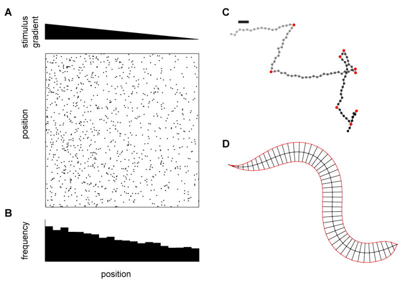
Different levels of behavioral metrics. (A) Tactic behaviors cause animals to migrate up or down gradients of some environmental cue. Here we examine the case of tracking C. elegans to measure a tactic behavior. The top triangle represents a gradient in stimulus magnitude, and each dot in the field below represents an instantaneous center of mass position of a worm in the gradient. On this scale, dot diameters are roughly the size of the worm. (B) In steady state, the distribution of worm positions over the gradient can be measured as an index or as a full distribution. Such measurements can also be made over time, incorporating transient changes in distribution. (C) At a finer scale, each worm’s track can be reconstructed in order to extract out the statistics of the worm’s coarse movements, including speed, heading, and, for instance, turning events. Turns are marked in red, gray dots represent early locations, black later locations, and the bar represents a worm’s body length. The integration over time of relevant statistics at this level should result in the distribution measured in (B). (D) More finely still, the shape of the worm’s bending over time can be analyzed to extract patterns in muscle activation. These patterns must ultimately result in the statistics in (C) and the distribution in (B).

In an ideal experimental strategy, behavioral (or neural) output is measured in a manner that accurately captures all the information it contains. However, in unrestrained animals, such datasets can be hard to obtain and challenging to analyze, particularly if multiple animals are interacting (Branson et al., 2009). It is therefore often necessary to constrain the animal’s behavior to a limited set of outcomes or to reduce the dimensionality of behavior. This can be done either by intuitively electing to focus on specific behavioral outputs or by applying more general data dimensionality reduction techniques like principal component analysis (PCA). A key question then becomes how to perform this dimensionality reduction without losing important circuit outputs. An ideal version of this transformation would minimize the loss of relevant information and eliminate redundancy and noise from the signal. While it is not necessary to preserve all information in the behavior, it is essential to preserve the part of the behavioral signal that is related to the input stimulus. In practice, a few metrics can be used to assess the preservation of relevant information. For example, it is possible to quantify how much the input stimulus is predictive of the behavioral output by computing the correlation or mutual information between these two signals (Lewi et al., 2011; Machens, 2002). Similarly, the extent to which an input is correctly predicted by the output (an approach that is limited by the quality of one’s predictive model) is another useful metric (Bialek and Rieke, 1992; Bialek et al., 1991). Computing these metrics allows for the assessment of the relative quality of different behavioral or neural representations and makes it significantly easier to compare behavioral phenotypes.

How can one address feedback from behavioral outputs to sensory inputs?

As we have discussed so far, circuits involved in sensorimotor transformation can be studied in an entirely reactive mode: a stimulus is provided, and a behavioral output is evoked. Yet because the animal is often restrained, the behavioral output has no impact on the animal’s subsequent sensory experience. This framework breaks the natural feedback of an animal’s behavioral output on its perception, preventing the statistics of the sensory environment from being altered in the way that evolution and experience has entrained in the circuit. Because the feedback loop is broken, these experiments are called “open loop”. While breaking the feedback loop has its place, being able to understand and manipulate feedback loops is important for understanding the circuit. Given that sensorimotor circuits normally use such feedback, it is critical to know how uncoupling behavior from perception might produce misleading answers. Finally, “awake and behaving” brains are in a different neuromodulatory state from those in a passive, restrained animal, altering the responses of sensory circuits in ways that can be general (corresponding to arousal) or specific (altering, for example, the tuning properties of specific neurons). Here we outline some of these effects, and then consider ways of manipulating feedback between sensory inputs and behavioral outputs.

An animal’s sensory strategy can be tuned according to its motor output. As it moves, it displaces its sensory organs in some spatiotemporal pattern, imposing this sampling pattern on the observations of the natural world. The brain has access to information about these movement patterns in two ways, both statistically over time and on a trial-by-trial basis, through proprioceptive sensors and circuits that return efferent copies of motor commands to sensory systems. For example, recent work has demonstrated that the gain of motion-sensitive cells in the fly visual system is dynamically adjusted by transient bouts of either walking or flying, boosting responses to more rapid motion stimuli (Chiappe et al., 2010; Jung et al., 2011; Maimon et al., 2010). Analogous results have been described in fish (Ahrens et al., 2012) and in mice (Niell and Stryker, 2010), and are broadly consistent with longstanding observations in awake, behaving primates (Reynolds and Chelazzi, 2004). Whether these specific signals represent different brain states, in which the activities of many neurons are altered, or whether these signals reflect targeted modulations of neurons whose outputs are of particular relevance to movement (such as neurons that detect visual motion) remains unclear.

A variety of efforts have established “virtual reality” environments in which the experimentalist captures the intended movements of the animal while it is immobilized or restrained, and uses this information to alter the sensory world to reflect its intended movement (reviewed in (Dombeck and Reiser, 2012)). Such “closed loop” systems were pioneered in flies and have been used to examine innate behavioral responses to visual (Goetz, 1968) and olfactory signals (Duistermars and Frye, 2008). Analogous systems have been implemented for mice, allowing full, three-dimensional reconstructions of virtual visual worlds (Harvey et al., 2009). These systems allow manipulation of the natural relationship between sensory inputs and motor output and also facilitate simultaneous monitoring of neural activity and behavior. In addition, while obtaining real time feedback from an immobilized animal provides one means of closing the behavioral loop, it is also possible to systematically explore open and closed loop regimes by tracking a freely moving animal and displacing the sensory world in real time (Fry et al., 2004; Schuster et al., 2002; Strauss and Heisenberg, 1990). Alternatively, one can reopen the loop between sensory input and behavioral output in a freely moving animal by adjusting the sensory environment around it so as to remove the effects on the input that would have been produced by its motor output (Fry et al., 2008, 2009). Finally, experiments in zebrafish have gone one step further in decoupling behavioral output from sensory input. In these experiments, fish were paralyzed, and motor neuron signals were monitored; from these signals, swim movements were decoded and used to control the sensory input (Ahrens et al., 2012; Portugues and Engert, 2011).

What can we hope to learn from dynamically manipulating the feedback between movement and sensation? At one extreme, neural circuit function might be fundamentally different when an animal is behaving versus quiescent and may depend on the type of behavior performed (e.g., flying or walking). Fortunately for much of the work that has been done in sensory neuroscience, this extreme does not seem to closely match reality: while the tuning properties of specific cells change in response to behavioral activity, the core features of these responses are apparent in the non-behaving animal (Clark et al., 2007; Ferezou et al., 2006; Maimon et al., 2010). However, when experiments are conducted in open loop conditions, where the sensory input is well-controlled but independent of behavior, the observed behavioral responses might be shaped not only by the sensory input but also by the discrepancy between it and the expected input given the behavioral modulation. A virtual reality environment can eliminate these discrepancies, but can also accentuate them, enabling exploration of circuit function under a broad range of conditions. These studies can reveal what elements of behavioral feedback a circuit is sensitive to, facilitating the description of the computation it performs. In addition, there are undoubtedly circuits that largely encode information in relation to efferent copies of the animal’s movements, and compute, for example, error signals between the sensory inputs an animal receives and those it expects (Boyden and Raymond, 2003; Portugues and Engert, 2011). While such circuits could be rare, information about the ongoing behavior of the animal is likely relayed to many levels of each sensory system, affecting many neurons, and what differs is the granularity and extent to which a given neuron’s response is dominated by sensory input versus behavioral output.

What is the goal of circuit manipulation?

With informative stimuli and behavioral metrics in hand, the ultimate goal when examining a circuit is to understand how the circuit components contribute to the sensorimotor transformation. Genetic tools that manipulate circuits can provide causal links between neural activity and behavioral output, an invaluable contribution to understanding circuit function. Cell-type specific expression of proteins allows constitutive or acute activation or inactivation of neurons by light, temperature, or drugs in worms, flies, fish, and mice (Bernstein and Boyden, 2011; England, 2010; Fenno et al., 2011; Luo et al., 2008; Miesenbock, 2009; Venken et al., 2011; White and Peabody, 2009). Having independent control over each synaptic input to a cell while providing a stimulus and monitoring behavior would allow one to attribute particular behavioral and computational roles to specific synapses. While such tools are not broadly available, exciting steps in this direction are underway (Ibanez-Tallon and Nitabach, 2012; Levitz et al., 2013; Szobota and Isacoff, 2010). More modestly, one can envision artificially controlling the activity of a neuron, reproducing exactly its native temporal activity and statistics in the context of a particular stimulus and then deviating from it. While this is, in principle, possible using optogenetic tools, such a systematic exploration has not yet been done. Fortunately, cruder experiments that either silence or ablate neurons, or increase their activities independent of their synaptic inputs, can provide many useful insights. Regardless of the granularity of the genetic manipulation of neural activity, it is critical to minimize the opportunities for a circuit to adapt or compensate, either developmentally or physiologically. In particular, adaptive changes in circuit function on the timescale of milliseconds to minutes are essentially unavoidable and might arguably reflect the dynamics of sensorimotor processing. However, circuit changes that reflect modulation of gene expression or synaptic connectivity and morphology over longer time-scales are largely undesirable. Therefore, the most interpretable experiments implement acute changes in neural activity and rapidly read out circuit function.

Neurons can be either activated or inactivated by genetic manipulation. At first glance, inactivation would appear to be the simpler manipulation, since there are relatively few ways to be ‘inactive’. However, existing tools for inactivation are not equivalent to voltage clamps that chain neurons exactly to their resting potentials. Typical tools either tonically or transiently hyperpolarize a neuron or physically prevent synaptic release. For spiking neurons, if one can ignore sub-threshold effects on membrane potential, and ignore electrical synapses and extracellular effects, either of these manipulations should be equivalent to enforcing a 0 Hz firing rate (a condition called ‘silencing’). On the other hand, for graded potential neurons, both of these manipulations are more problematic since there is no natural minimum activity equivalent to 0 Hz. Nevertheless, in both spiking and non-spiking cases, “inactivation” really means setting the output to be constant and low, a condition that is likely to be substantially different from that seen in the intact circuit.

For neuronal activation, genetic tools can depolarize cells and directly increase intracellular calcium. Again, if electrical synapses can be ignored, these are functionally comparable manipulations. For both spiking and non-spiking cells, one might hope that constitutive activation entails setting a constant, high level of synaptic output. However, given both cellular and network dynamics, many of these manipulations likely produce unstable increases in activity. Nonetheless, many of these manipulations have defined circuit elements sufficient to evoke behaviors, but it is important to note that neurons that require precise activation protocols to drive behavior would have been missed.

The issues surrounding single cell manipulations lead to the question of how one should interpret silencing or activation experiments in the context of networks. How comparable is the network activity in the artificially activated case compared to natural activation? And conversely, during silencing, is it merely as if the affected neuron is removed from the network? For example, in the simplest case, neurons are perfectly linear, and thus the effects of silencing or activation are easily interpretable (Figure 3A, B). However, common regulatory mechanisms, such as gain control or adaptation could wreak havoc with manipulation experiments (Figure 3C, D). While rapid feedback is likely to affect the outcome of many circuit perturbations, adaptation seems more likely to arise with longer timescale manipulations, such as the thermal activation and inactivation methods often used in Drosophila(Kitamoto, 2001; Rosenzweig et al., 2005). Brief perturbations that can be applied on the same timescale as natural network activity, such as the ones enabled by optogenetics, should give the most insight into a neuron’s contribution to the network. Neural circuits have necessarily evolved to be robust to natural perturbations (such as injuries) and flexible (to accommodate variable environments), however these redundant or distributed forms of processing may make the effects of experimental manipulation difficult to characterize. This suggests that although extreme manipulations (such as eliminating more than one cell type or leaving activity intact in only one of many cell types) may be advantageous, they also increase the likelihood that compensatory mechanisms shape the resulting output.

Figure 3.

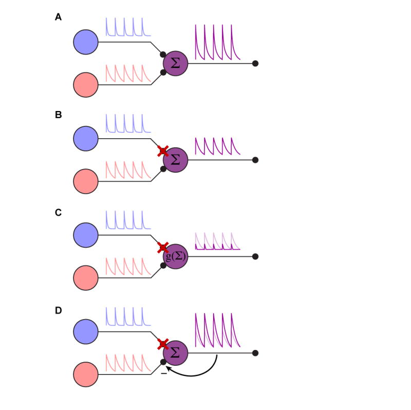
Circuit manipulation. (A) Cartoon of a simple, intact circuit. The purple cell simply sums the synaptic input from the red and blue cells. (B) Illustration of a simply interpretable silencing outcome. When the blue cell is silenced, the purple cell now simply reports the red cell’s activity. The entire system is linear in this case. (C) Illustration of dynamic range confounding interpretation. In this case, when the blue cell is silenced, the lack of a tonic blue input moves the purple cell below its natural dynamic range, clipping the remaining input. This is the equivalent of putting a nonlinearity g(.) on the summation of the inputs. The linear case is shown in light purple for comparison. (D) Illustration of feedback gain confounding interpretation. In this case, the inputs are summed, but the purple cell provides negative feedback on the gain from the red and blue cells. When the blue cell is silenced, the gain on the red synapse is increased to accommodate the lesser total input. The linear case is shown in light purple for comparison. Cases (C) and (D) illustrate complications to interpreting silencing experiments in even very simple circuits; similar caveats will apply to activation experiments.

Ultimately, one should compare the perturbed network’s activity to a model’s predictions. A strong model predicts both the activity of the unperturbed network and the effects of perturbations. Furthermore, since removing a neuron’s output could have strong and counter-intuitive effects on circuit function if feedback mechanisms are prominently involved, models that incorporate feedback could be critical when interpreting how discrete manipulations of circuit components influence behavior.

What is in a model?

Given the complexity of the brain, models of circuit function are of paramount importance and can serve two valuable purposes. First, a model can provide a test of sufficiency. Is a certain set of assumptions and mechanisms sufficient to produce the observed measurement of circuit activity or behavioral response? Second, a model can generate testable experimental hypotheses by suggesting other phenomena produced by these assumptions. Biological models fall into two broad classes. One class of models is detail-oriented, incorporating as much of the available data about individual circuit components as possible, with the goal of achieving verisimilitude. In these “realistic” models, additional parameters that capture more of the biology are useful. The model becomes a mirror for the biological system, and its value lies chiefly in its ability to explore parameters and predict results of novel experiments. Likewise, it provides mechanistic explanations for observed phenomena by permitting simulation of the dynamics of contributing components. For example, a model of this type captures the responses of insect photoreceptors to light, providing new insights into how these cells efficiently represent information across light levels (Song et al., 2012). An alternative type of model is phenomenological, seeking to derive the simplest construct that produces a particular feature of a stimulus-response relationship. Such models can be derived from experimental data or can emerge from first principles considerations of a circuit’s objectives and constraints (Bialek, 1987; Field, 1994; Hassenstein and Reichardt, 1956; Hateren, 1992; Laughlin, 1981; Srinivasan et al., 1982). In this case, the model may not provide verisimilitude across a broad range of conditions and the specific features of the model are not exact representations of how the brain works. Rather, this kind of model describes some set of phenomena and provides a potential explanation for them. A popular example is the LN model (Figure 1C), which gives intuition about the dynamics and range of a response without referencing biological details of how the linear and non-linear features arise. At the same time, phenomenological models like the LN framework have been widely used because the individual components of the model, like a saturating non-linearity, are biologically plausible.

Realistic versus phenomenological models offer particular tradeoffs. By their nature, phenomenological models have fewer parameters and fewer equations. Thus, they are more likely to be analytically tractable, allowing one to easily examine how responses vary as a function of different inputs. Likewise, parameter space, and interactions between parameters, can be easily explored. However, parameters in phenomenological models may be difficult to map directly onto biological processes, making them less useful for exploring mechanistic details. Indeed, such a model may capture a circuit algorithm, even when it is difficult to map the biophysical implementation onto model parameters. Moreover, perhaps more usefully, a successful phenomenological model would correctly predict responses of a circuit to novel stimuli, suggesting informative experiments. Conversely, while the parameters of a realistic model may provide insight into how the biophysical and network details give rise to function, it may give little insight into the computation that takes place. As many circuits may implement the same high-level computations via different molecular mechanisms (Marder and Goaillard, 2006), both the algorithmic and implementation details of circuits are important to model. Furthermore, as models become more complex and require numerical integration, it becomes harder to intuitively appreciate the relationship between a model’s predictions and its parameters. There is thus a spectrum of models, ranging from the simple and analytic to the complex and numerical, often trading intuition for a more exact representation of the system. Given the tradeoffs, the goals of a model should be considered carefully when deciding what to incorporate into it. Broadly speaking, the simplest model that explains the data is desirable. However, since there is no clear definition of “simple”, choosing the simplest model is often a matter of taste and the relative importance of defined biological mechanisms will be critical. Finding the fewest parameters necessary to fit the data clearly offers advantages, but fit quality itself can also be defined in many ways, depending on the purpose of the model.

The continuum of levels of understanding a circuit, from algorithm to neural instantiation to biophysical machinery (Figure 4), also lends itself to a continuum of modeling structures (Marr, 1982). At a high level, the aim is to map the phenomenology of a circuit, showing how it translates input to output and how that output serves the animal (e.g., (Goetz, 1968)). At a more detailed level, the algorithms employed by the circuit to produce the phenomena are identified and define the mathematical operations required to transform the circuit inputs into its outputs (e.g., (Hassenstein and Reichardt, 1956)). As the model takes into account greater detail, the hope is to assign algorithmic operations to particular circuit components (e.g., (Olsen and Wilson, 2008)). At a biophysical level, one could model how an individual neuron’s channels, spatial arrangement of synapses, morphology, cellular compartments, and excitability contribute to its input-output functions within the circuit (e.g., (Herz et al., 2006)). An important long-term goal of circuit dissection efforts is to link models at different levels in this hierarchy. However, as one progresses from top to bottom in this framework, redundancy and distributed computations make mapping algorithms onto specific lower level components a daunting problem. Conversely, as one progresses from bottom to top, the higher levels must increasingly make use of coarse-grained versions of the low level details, which are displaced in favor of quantitative summaries. For instance, the representation of a synapse in a neural network model may have very different features, depending on the level at which the network is described. A detailed model of transmission between two neurons might capture the dynamic, stochastic nature of synaptic vesicle release. A higher-level model of the interactions in a network, on the other hand, may incorporate a concise mathematical description of the synapse that only captures the average effect of vesicle release and depletion. In moving from the top level downward, one broad challenge lies in identifying required algorithmic steps that can be sought in lower level elements of the circuit. In moving from the bottom level upwards, a second challenge lies in discovering the principled ways to summarize the low-level details as models capture ever-larger aspects of circuit function. The generation of these types of models is essential to truly understand and test how circuits work.

Figure 4.

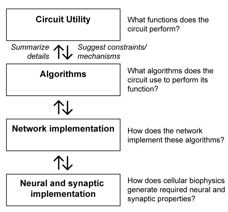
A hierarchy of levels of understanding neural computation. Modeling, detailed behavioral analysis, stimulus selection, neural manipulations, and neural measurements feed into understanding at all these levels. Moving up through the hierarchy, one goal is to connect the broader description to the low-level details. Moving down through the hierarchy, one goal is to use the broader descriptions to suggest mechanisms or constraints that might be sought in the lower levels.

Conclusions

The logic and language of genetics have provided innumerable insights into gene function. Genetic tools that modulate the activity of targeted neurons have inspired the application of logically equivalent approaches to circuits. These studies add critical elements to our understanding, creating maps that describe causal links between neurons and behaviors of interest. However, this is not necessarily the ultimate goal of circuit dissection. Much as biochemical, biophysical, and computational approaches provide new insights into the arrow diagrams of geneticists, understanding the relationships between stimulus space, behavioral responses, and the dynamics of neuronal activity will be necessary to unravel the mechanisms of neural computation. By exploring circuits that perform similar sensorimotor transformations in different model systems, spanning a broad expanse of phylogeny, these studies will reveal the constraints under which fundamental neural computations have evolved. Finally, given new efforts to map neural activity on large scale and to simulate the human brain in silico(Alivisatos et al., 2013; Markram, 2006) building the considerations we have outlined here into experimental design will be critical to understanding circuits on grand scale.