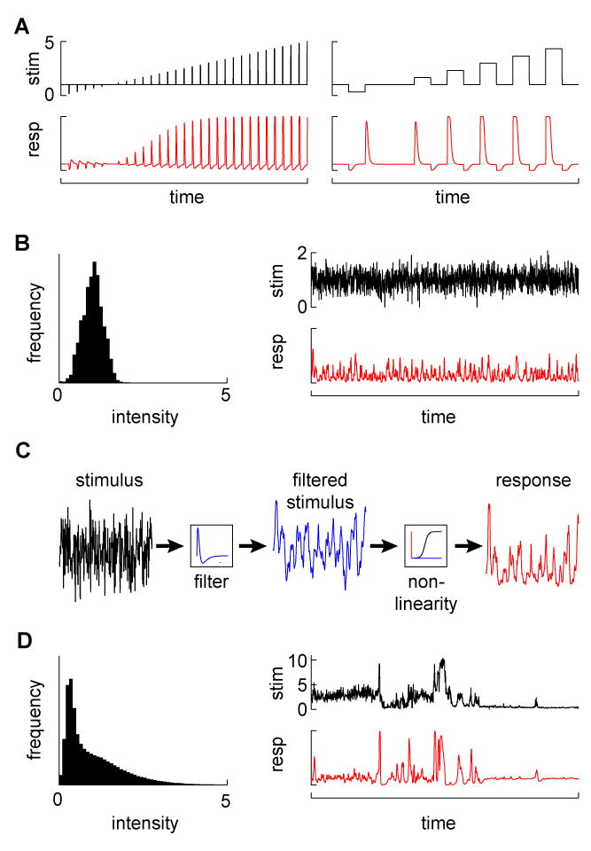
Figure 1.

Probing a system with different stimuli. (A) Examples of pulse and step changes in stimuli (top) and simulated responses (bottom). (B) A Gaussian stimulus. The left plot shows the distribution of Gaussian stimulus values (with mean 1), while the right plots show a Gaussian noise stimulus (top) and a simulated sample response (bottom). (C) Explanation of the LN model. In the model, stimuli (left trace) are first passed over with a linear filter to produce a weighted average of the stimulus (middle trace). That filtered stimulus is mapped onto the response (right trace) with a function that may contain non-linearities. The filter can be estimated from the system response to a Gaussian noise input, after which the mapping function can be fit to the data. The function is linear in the case of the linear system, or can account for post-filtering non-linearities that occur quickly compared to the filtering process, for instance to prevent very strong responses (create saturation) or to prevent negative responses (create rectification). (D) A natural stimulus (from (Van Hateren, 1997)). In the distribution on the left, note the infrequent but large stimulus values (the mean is set to 1). A natural time series of that distribution, incorporating naturalistic dynamics (top), along with a simulated sample response to that stimulus (bottom).