A generative probability model of joint label fusion for multi-atlas based brain segmentation

Abstract

Automated labeling of anatomical structures in medical images is very important in many neuroscience studies. Recently, patch-based labeling has been widely investigated to alleviate the possible mis-alignment when registering atlases to the target image. However, the weights used for label fusion from the registered atlases are generally computed independently and thus lack the capability of preventing the ambiguous atlas patches from contributing to the label fusion. More critically, these weights are often calculated based only on the simple patch similarity, thus not necessarily providing optimal solution for label fusion. To address these limitations, we propose a generative probability model to describe the procedure of label fusion in a multi-atlas scenario, for the goal of labeling each point in the target image by the best representative atlas patches that also have the largest labeling unanimity in labeling the underlying point correctly. Specifically, sparsity constraint is imposed upon label fusion weights, in order to select a small number of atlas patches that best represent the underlying target patch, thus reducing the risks of including the misleading atlas patches. The labeling unanimity among atlas patches is achieved by exploring their dependencies, where we model these dependencies as the joint probability of each pair of atlas patches in correctly predicting the labels, by analyzing the correlation of their morphological error patterns and also the labeling consensus among atlases. The patch dependencies will be further recursively updated based on the latest labeling results to correct the possible labeling errors, which falls to the Expectation Maximization (EM) framework. To demonstrate the labeling performance, we have comprehensively evaluated our patch-based labeling method on the whole brain parcellation and hippocampus segmentation. Promising labeling results have been achieved with comparison to the conventional patch-based labeling method, indicating the potential application of the proposed method in the future clinical studies.

1. Introduction

With the advent of magnetic resonance (MR) imaging technique, image analysis on MR images plays a very important role in quantitatively measuring the structure difference between either individuals or groups (Fennema-Notestine et al., 2009; Paus et al., 1999; Westerhausen et al., 2011). In many neuroscience and clinic studies, some regions-of-interest (ROIs), e.g., hippocampus, in the human brain are specifically investigated due to their close relation to brain diseases such as dementia (Devanand et al., 2007; Dickerson et al., 2001; Holland et al., 2012). Consequently, automatic accurate labeling and measurement of anatomical structures become significantly important in those studies to deal with large amount of clinical data. However, automatic labeling still remains a challenging problem because of the complicated brain structures and high inter-subject variability across individual brains.

Recently, patch-based labeling methods have emerged as an important direction for the multi-atlas based segmentation (Coupe et al., 2011; Rousseau et al., 2011; Wang et al., 2012; Wang et al., 2011; Yan et al., 2013). The basic assumption in these methods is that, if two image patches are similar in appearances, they should have the same anatomical label (Rousseau et al., 2011). Most patch-based labeling methods perform label fusion in a non-local manner. Specifically, to label a patch in the target image, all possible candidate patches from different atlases are considered, with their contributions weighted according to the patch similarities w.r.t. the target patch. In this way, these non-local based labeling methods can alleviate the influences from the possible registration errors.

Although patch-based labeling methods are effective in many applications, they still have several limitations:

• (1)All candidate patches from atlases contribute to the label fusion, according to their similarities to the target patch. However, even the atlas patches with high appearance similarity could still bear the wrong labels, thus undermining the label fusion result due to the lack of power in suppressing the misleading patches.
• (2)If a majority of candidate patches have wrong labels, those patches will dominate the conventional label fusion procedure and lead to incorrect labeling results (Wang et al., 2012). The reason is that most label fusion methods independently treat each candidate patch during label fusion, thus allowing those highly correlated candidate patches to repeatedly produce the labeling errors.
• (3)The weights calculated from patch appearance are often directly applied for label fusion. Although these weights are optimal for patch representation, i.e., making the combination of candidate patches close to the target patch, these weights are not necessarily optimal for label fusion.
• (4)Most current label fusion methods complete the label fusion right after sequentially labeling each image point in the image domain, thus lacking a feedback mechanism to help correct possible labeling errors.

In this paper, we propose a novel patch-based labeling method, where a generative probabilistic model is presented to predict the labels based on the observations of registered atlas images. Specifically, the goals are (1) to seek for the best representation of the underlying target patch from a set of similar candidate atlas patches, and (2) to achieve the largest labeling consensus, among the entire candidate atlas patches, in predicting the label for each target point. For the first goal, we introduce the concept of sparse representation (Tibshirani, 1996; Vinje and Gallant, 2000; Zhang et al., 2012a, 2012b, 2012c) by imposing a non-Gaussian sparsity prior (Seeger et al., 2007; Seeger, 2008) on the label fusion weights. Thus, our method, equipped with sparsity constraint, is able to alleviate the issue of ambiguous patches by representing each target patch with only a small number of atlas patches, instead of all candidate atlas patches. For the second goal, we propose to measure the labeling unanimity through the joint probability of patch dependencies, which encodes the risk for any pair of candidate patches to produce labeling error simultaneously. In our probability model, we describe the dependency probability in two ways. First, we measure the pairwise correlation of morphological error patterns for any pair of candidate patches, in order to penalize those candidate patches with simultaneously incorrect labels. Second, we further inspect whether the latest label fusion result achieves the largest labeling consensus among the candidate patches. Since the estimation of dependency probability is related with the currently estimated labels, our label fusion method offers the feedback mechanism by iteratively improving the label fusion result with the gradually refined estimation of the dependency probability. To this end, we present an efficient EM-based solution to infer the optimal labels for the target image.

In terms of joint label fusion, our work is close to (Wang et al., 2012), which also measured the joint labeling risk between two patches. However, our generative probability model has several unique improvements. First, the joint distribution of patch dependency is measured by not only the error pattern but also the labeling consensus w.r.t. the latest estimated label. Second, the label fusion method in (Wang et al., 2012) lacks of the feedback mechanism as in our method to examine the current label fusion result and further refine the estimation of dependency. Third, our method takes advantages of sparsity constraint to obtain robust label fusion results to suppress misleading patches. As we will point out later, our method can be regarded as a generalized solution of most existing patch-based labeling methods (Artaechevarria et al., 2009; Coupe et al., 2011; Rousseau et al., 2011; Tong et al., 2012; Zhang et al., 2012a).

We demonstrated the labeling performance on NIREP-NA0 dataset (Christensen et al., 2006) with 32 manually delineated ROIs and also the ADNI (Alzheimer's Disease Neuroimaging Initiative) dataset with manually labeled hippocampi. Compared to the conventional patch-based labeling method (Coupe et al., 2011; Rousseau et al., 2011), our method achieves more accurate labeling results on both datasets. In the following, we first present our novel generative probability model for label fusion in Section 2. Then, we evaluate it in Section 3, by comparison with the conventional patch-based methods. Finally, we conclude the paper in Section 4.

2. Method

Let S be the set of N atlas images I = {I_k|k = 1, …, N} and their corresponding label maps L = {L_k|k = 1, …, N}, which have been already registered to the target image T (that will be labeled) by linear/non-linear registration methods (Vercauteren et al., 2008, 2009; Wu et al., 2013, 2007, 2012a, 2010). For each point ν ∈ Ω_Ik, ${\stackrel{\rightharpoonup }{L}}_k\left(v\right)$ is a binary vector of {0, 1}^M representing the particular label at the point ν, where M is the total number of labels. The goal of label fusion is to propagate the labels from the registered atlases to the target image T. For each point u ∈ Ω_T in the target image T, its label ${\stackrel{\rightharpoonup }{L}}_T\left(u\right)$ will be estimated through the interaction between the target patch ${\mathcal{P}}_T\left(u\right)$ centered at point u and all possible candidate patches ${\mathcal{P}}_k\left(v\right)$ at the registered atlas image I_k. The spatial location v is usually confined to a relatively small neighborhood n(u) ⊂ Ω_T. Given the weight w_k(u, v) for the pair of ${\mathcal{P}}_T\left(u\right)$ and ${\mathcal{P}}_k\left(v\right)$, we can estimate the label vector θ(u) for the target point u as

$$\stackrel{\rightharpoonup }{\theta }\left(u\right)=\frac{\sum _{k=1}^N\sum _{v\in n\left(u\right)}{w}_k(u,v)\cdot {\stackrel{\rightharpoonup }{L}}_k\left(v\right)}{\sum _{k=1}^N\sum _{v\in n\left(u\right)}{w}_k(u,v)}.$$ (1)

It is worth noting that $\left(\stackrel{\rightharpoonup }{\theta }\right(u)=[{\theta }^1\left(u\right),\dots ,{\theta }^m\left(u\right),\dots ,{\theta }^M\left(u\right)]$ is a vector of continuous likehood for each possible label at point u after label fusion. Then, the final label of the point u can be determined by binarizing the fuzzy assignment $\stackrel{\rightharpoonup }{\theta }\left(u\right)$ to a binary vector ${\stackrel{\rightharpoonup }{L}}_T\left(u\right)=\left[l^1\right(u),\dots ,l^m(u),\dots ,l^M(u\left)\right]$

$$l^m\left(u\right)=\{\begin{array}{cc}1,\hfill & \text{if}{\theta }^m\left(u\right)\text{has the highest value}\hfill \\ 0,\hfill & \text{otherwise}\hfill \end{array}\phantom{\}}.$$ (2)

In the following, we will first introduce the conventional patch-based labeling method with non-local averaging in Section 2.1. Then, we will present our generative probability model for label fusion in Section 2.2. The inference of probability model will be presented in Section 2.3, followed by the discussion in Section 2.4. Our whole method will be summarized in Section 2.5.

2.1. Conventional patch-based labeling method by non-local averaging

The principle of conventional patch-based labeling method is originated from the non-local strategy which is widely used in the computer vision area, such as image/video denoising (Buades et al., 2005) and super-resolution (Protter et al., 2009). The applications in medical images can also be found in (Awate and Whitaker, 2006; Manjón et al., 2011). The overview of patched-based method is shown in Fig. 1(a). Hereafter, for each target point u ∈ Ω_T, we use the column vector $\stackrel{\rightharpoonup }{y}$ to vectorize the target patch ${\mathcal{P}}_T\left(u\right)$ centered at u (red box in Fig. 1(a)). In order to account for the registration uncertainty, a set of candidate atlas patches (pink boxes in Fig. 1(a)) are included in a search neighborhood n(u) (blue boxes in Fig. 1(a)) from different atlas images. For clarity, we arrange each candidate patch ${\mathcal{P}}_k\left(v\right)$ into a column vector ${\stackrel{\rightharpoonup }{a}}_j$ and then assemble them into a dictionary matrix $\mathbf{A}={\left[{\stackrel{\rightharpoonup }{a}}_j\right]}_{j=1,\dots ,Q}$, where j = (k, v) is a bivariate index of particular candidate patch ${\mathcal{P}}_k\left(v\right)$ and Q = N · |n(u)| denotes the total number of candidate patches. Following the same order, we assemble the label vector ${\stackrel{\rightharpoonup }{L}}_k\left(v\right)$ of each candidate atlas patch into the label matrix, denoted by $\Lambda ={\left[{\stackrel{\rightharpoonup }{\lambda }}_j\right]}_{j=1,\dots ,Q}$. In the setting of non-local averaging, each candidate patch ${\stackrel{\rightharpoonup }{a}}_j$ contributes to label fusion. The non-local weight w_j in the column vector $\stackrel{\rightharpoonup }{w}={\left[w_j\right]}_{j=1,\dots ,Q}$ is related to the appearance similarity of patches

$$w_j=e^{-\frac{{\Vert \stackrel{\rightharpoonup }{y}-{\stackrel{\rightharpoonup }{a}}_j\Vert }^2}{{\tau }^2}},$$ (3)

where τ is the decay parameter (Coupe et al., 2011) controlling the strength of penalty in the exponential way. Given the weighting vector $\stackrel{\rightharpoonup }{w}$ for each point u, we are able to predict the label $\stackrel{\rightharpoonup }{\eta }={\stackrel{\rightharpoonup }{L}}_T\left(u\right)$ following Eqs. (1) and (2).

Fig. 1.

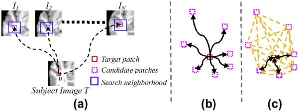
The overview of the patch-based labeling method in the multi-atlas scenario. As shown in (a), the reference patch (red box) seeks for contributions from all possible candidate patches (pink boxes) in a small search neighborhood (blue box). The graph demonstrations by non-local averaging and our method are shown in (b) and (c), respectively.

2.2. A generative probability model for patch-based label fusion

In this section, we first interpret the conventional patch-based label fusion methods in a deterministic probability model, which lacks of the dependency among candidate patches. Then, we propose to model the labeling dependency as the joint probability of all candidate patches in achieving the largest labeling consensus simultaneously. After integrating the labeling dependency, we further present a generative probability model to guide the label fusion procedure.

2.2.1. The probability model for conventional patch-based label fusion method

As we mentioned early, the procedures of estimating the weighting vector $\stackrel{\rightharpoonup }{w}$ and predicting label $\stackrel{\rightharpoonup }{\eta }$ are totally separated in the conventional label fusion methods. Thus, the objective in the conventional methods is to maximize the following posterior probability:

$$p(\stackrel{\rightharpoonup }{w}\mid \mathbf{A},\stackrel{\rightharpoonup }{y})\propto p(\mathbf{A},\stackrel{\rightharpoonup }{y}\mid \stackrel{\rightharpoonup }{w})p\left(\stackrel{\rightharpoonup }{w}\right)=p(\stackrel{\rightharpoonup }{y}\mid \mathbf{A},\stackrel{\rightharpoonup }{w})p(\mathbf{A}\mid \stackrel{\rightharpoonup }{w})p\left(\stackrel{\rightharpoonup }{w}\right).$$ (4)

Assuming the residual between $\stackrel{\rightharpoonup }{y}$ and A $\stackrel{\rightharpoonup }{w}$ follows Gaussian distribution the likelihood probability $p(\stackrel{\rightharpoonup }{y}\mid \mathbf{A},\stackrel{\rightharpoonup }{w})$ is defined as:

$$p(\stackrel{\rightharpoonup }{y}\mid \mathbf{A},\stackrel{\rightharpoonup }{w})\propto e^{-\frac{{\Vert \stackrel{\rightharpoonup }{y}-\mathbf{A}\stackrel{\rightharpoonup }{w}\Vert }^2}{{\tau }^2}},$$ (5)

where τ is related with the standard deviation of residual errors. Due to no prior knowledge on A, the conditional probabilities $p(\mathbf{A}\mid \stackrel{\rightharpoonup }{w})$ is simplified to follow the uniform distribution.

The label fusion methods with non-local averaging (Coupe et al., 2011; Rousseau et al., 2011) usually do not have the explicit constraint on prior $p\left(\stackrel{\rightharpoonup }{w}\right)$, which derives the calculation of weights (Eq. (3)) in the scenario of Maximum Likelihood (ML) estimation. Recently, sparse coding has been introduced in label fusion by imposing the sparsity constraint upon the label fusion weights $\stackrel{\rightharpoonup }{w}$ (Tong et al., 2012; Wu et al., 2012b; Zhang et al., 2012a). That is, the weighting vector $\stackrel{\rightharpoonup }{w}$ with a majority of elements approaching to zero is preferred a priori (Seeger et al., 2007). The sparsity constraint can be achieved by assuming the independent Laplace distribution to each element w_j in $\stackrel{\rightharpoonup }{w}$

$$p\left(\stackrel{\rightharpoonup }{w}\right)=\prod _{j=1}^{Q}p\left(w_j\right)\propto \prod _{j=1}^Q{e}^{-\rho w_j}=e^{-\rho \sum _{j=1}^Q{w}_j},$$ (6)

where ρ > 0 is a scalar parameter measuring the distribution diversity. It is worth noting that each weight is non-negative in Eq. (6), i.e., w_j ≥ 0(∀j). Intuitively, the probability of large w_j is much smaller than that of small w_j. Thus, the prior $p\left(\stackrel{\rightharpoonup }{w}\right)$, encourages the value of every element in $\stackrel{\rightharpoonup }{w}$ to approach to zero. Given the prior $p\left(\stackrel{\rightharpoonup }{w}\right)$, the optimization of Eq. (4) turns to the Maximum-a-Posteriori (MAP) problem

$$\widehat{\stackrel{\rightharpoonup }{w}}=\text{arg}\underset{\stackrel{\rightharpoonup }{w}}{\min }{\Vert \stackrel{\rightharpoonup }{y}-\mathbf{A}\stackrel{\rightharpoonup }{w}\Vert }_2^2+\rho {\Vert \stackrel{\rightharpoonup }{w}\Vert }_1,s.t.w_j\ge 0,\forall j\in \{1,\dots ,Q\},$$ (7)

which is also the well-known non-negative LASSO problem (Tibshirani, 1996).

The advantage of sparsity constraint is demonstrated in Fig. 2. In this example, we examine the candidate patches for the target patch (the pink patch in the top of Fig. 2), from each atlas image (I₁ to I₄) and in the respective searching neighborhoods (blue boxes). The last second row in Fig. 2 shows the weights for each candidate patch by non-local mean, where blue and red colors denote the candidate patches having different or same labels as the target patch, respectively. It is clear that some candidate patches, although having different labels, still have high patch similarity, which will mislead the label fusion procedure. The last row in Fig. 2 shows the weights computed by Eq. (7) (using the sparsity constraint). Since the sparsity constraint encourages using only a small number of candidate patches to represent the target patch, the influence from the misleading patches is suppressed, as observed with very fewer blue spikes in the last row of Fig. 2. In this way, our label fusion method can be a_i more robust than non-local mean.

Fig. 2.

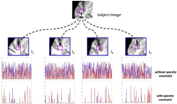
The advantage of using sparsity constraint in label fusion. The last two rows show the weights between the target patch (the pink box in the top) and all possible candidate patches (selected from the searching neighborhood of each atlas image), computed by the non-local mean and the sparse constraint, respectively. The blue and red colors in the last two rows denote the candidate patches with different or same label as the target patch.

Graphic model is a useful tool in describing conditional dependence structure between random variables (Koller and Friedman, 2009). The graphic model of Eq. (7) is shown in Fig. 3(a). It is clear that the estimation of the label $\stackrel{\rightharpoonup }{\eta }$ is separated from the optimization of $\stackrel{\rightharpoonup }{w}$. In the following, we will propose a generative probability model by introducing the patch dependency probability next.

Fig. 3.

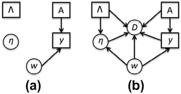
The graphic model of conventional patch-based method and our joint labeling method.

2.2.2. Modeling the labeling dependency of candidate patches in label fusion

As mentioned above, one limitation in the conventional patch-based label fusion method is that each candidate patch a_j is independently considered. To address this issue, we propose to model the dependency as the joint probability of candidate patches A that achieve the highest labeling accuracy simultaneously. In order to make our model tractable, we measure the pairwise probability of labeling dependency by any pair of candidate patches. Here, we use the variable D = {d_ij|i, j = 1, …, Q} to denote the pair of patches a_i and a_j which both label the target point u correctly. Then, the dependency probability p(d_ij) indicates the likelihood of making such agreement between a_i and a_j in label fusion.

Although it is difficult to directly estimate the dependency probability p(d_ij), we can learn its conditional probability in two ways. First, given the observations A, Λ and the target patch $\stackrel{\rightharpoonup }{y}$, we regard that the conditional probability $p(d_{\mathit{ij}}\mid \mathbf{A},\Lambda ,\stackrel{\rightharpoonup }{y})$ is related with the correlation of morphological error patterns (w.r.t. $\stackrel{\rightharpoonup }{y}$) of each pair of a_i and a_j. To this end, two patches a_i and a_j have high chance to produce similar labeling error only if (1) their error patterns, i.e., $e_i=(a_i-\stackrel{\rightharpoonup }{y})$ and $e_j=(a_j-\stackrel{\rightharpoonup }{y})$, are highly correlated, (2) they bear the same labels, i.e., $\delta ({\lambda }_i-{\lambda }_j)=1$, where δ(.) is the Dirac pulse function (δ(0) = 1), and (3) the magnitudes of error patterns, i.e., both ${\Vert e_i\Vert }_2^2$ and ${\Vert e_j\Vert }_2^2$, are large. Thus, the conditional probability $p(d_{\mathit{ij}}\mid \mathbf{A},\Lambda ,\stackrel{\rightharpoonup }{y})$ is given by penalizing the above pairwise mislabeling risk as:

$$\begin{array}{cc}\hfill & p(d_{\mathit{ij}}\mid \mathbf{A},\Lambda ,\stackrel{\rightharpoonup }{y})\propto e^{-{\beta }_1{\varphi }_{\mathit{ij}}^A},\text{and}\hfill \\ \hfill & {\varphi }_{\mathit{ij}}^A=\delta ({\stackrel{\rightharpoonup }{\lambda }}_i-{\stackrel{\rightharpoonup }{\lambda }}_j)\cdot [{\Vert e_i\Vert }_2^2\cdot [\mathit{NCC}(e_i,e_j)+1]\cdot {\Vert e_j\Vert }_2^2],\hfill \end{array}$$ (8)

where NCC(e_i, e_j) is the normalized cross-correlation between e_i and e_j. β₁ > 0 is a scalar controlling the penalty for the pair of patches ${\stackrel{\rightharpoonup }{a}}_i$ and ${\stackrel{\rightharpoonup }{a}}_j$ simultaneously making labeling errors.

Second, given the label fusion result $\stackrel{\rightharpoonup }{\eta }$ on the target point u, we can examine whether the estimation $\stackrel{\rightharpoonup }{\eta }$ achieves the largest labeling consensus between any pair of label ${\stackrel{\rightharpoonup }{\lambda }}_i$ on patch ${\stackrel{\rightharpoonup }{a}}_i$ and label ${\stackrel{\rightharpoonup }{\lambda }}_j$ on patch ${\stackrel{\rightharpoonup }{a}}_j$ Then the conditional probability $p(d_{\mathit{ij}}\mid \stackrel{\rightharpoonup }{\eta })$ is given as:

$$p(d_{\mathit{ij}}\mid \stackrel{\rightharpoonup }{\eta })\propto e^{-{\beta }_2{\varphi }_{\mathit{ij}}^{\Lambda }},\text{and}{\varphi }_{\mathit{ij}}^{\Lambda }=1-\frac{\delta ({\stackrel{\rightharpoonup }{\lambda }}_i-\stackrel{\rightharpoonup }{\eta })+\delta ({\stackrel{\rightharpoonup }{\lambda }}_j-\stackrel{\rightharpoonup }{\eta })}{2},$$ (9)

where β₂ > 0 is the scalar. It is apparent that $p(d_{\mathit{ij}}\mid \stackrel{\rightharpoonup }{\eta })$ has the lowest probability only if both candidate patch ${\stackrel{\rightharpoonup }{a}}_i$ and ${\stackrel{\rightharpoonup }{a}}_j$ bear different labels against $\stackrel{\rightharpoonup }{\eta }$. Here, we go one step further that the labeling dependency d_ij is also related with the weights w_i and w_j. Combining Eqs. (8) and (9), we define the conditional dependency probability $p(d_{\mathit{ij}}\mid \mathbf{A},\Lambda ,\stackrel{\rightharpoonup }{y},\stackrel{\rightharpoonup }{\eta },\stackrel{\rightharpoonup }{w})$ as:

$$p(d_{\mathit{ij}}\mid \mathbf{A},\Lambda ,\stackrel{\rightharpoonup }{y},\stackrel{\rightharpoonup }{\eta },\stackrel{\rightharpoonup }{w})\propto e^{-w_j{\varphi }_{\mathit{ij}}{w}_j},\text{and}{\varphi }_{\mathit{ij}}=(1-r){\varphi }_{\mathit{ij}}^A+r{\varphi }_{\mathit{ij}}^{\Lambda },$$ (10)

where β = β₁β₂ and 0 ≤ r ≤ 1 is the scalar balancing the impacts of ${\varphi }_{\mathit{ij}}^{\mathrm{A}}$ and ${\varphi }_{\mathit{ij}}^{\Lambda }$ during label fusion. As we will explain later r = 0 in the beginning since there is no estimation of $\stackrel{\rightharpoonup }{\eta }$ at that moment, and the degree of r will gradually increase to 0.5 at the end of label fusion procedure. Thus, the goal of our label fusion method is to seek for the representative candidate patches with not only the best representation for the target patch $\stackrel{\rightharpoonup }{y}$ but also the largest joint labeling consensus, which is described in a generative model next.

2.2.3. A generative probability model for joint patch-based label fusion

Given the observations $\mathcal{H}=\{\mathbf{A},\Lambda ,\stackrel{\rightharpoonup }{y}\}$, we aim to infer the model parameters $\Theta =\{\mathit{D},\stackrel{\rightharpoonup }{w},\stackrel{\rightharpoonup }{\eta }\}$ from the joint probability $p(\mathcal{H},\Theta )$

$$(\widehat{\mathit{D}},\widehat{\stackrel{\rightharpoonup }{w}},\widehat{\stackrel{\rightharpoonup }{\eta }})=\text{arg}\underset{(\stackrel{\rightharpoonup }{w},\stackrel{\rightharpoonup }{\eta })}{\max }p(\mathcal{H},\Theta ),s.t.w_j\ge 0,\forall j,$$ (11)

where the joint probability $p(\mathcal{H},\Theta )$ can be further decomposed as

$$\begin{array}{cc}\hfill p(\mathcal{H},\Theta )& =p(\mathit{D}\mid \mathbf{A},\Lambda ,\stackrel{\rightharpoonup }{y},\stackrel{\rightharpoonup }{w},\stackrel{\rightharpoonup }{\eta })p(\stackrel{\rightharpoonup }{y}\mid \mathbf{A},\Lambda ,\stackrel{\rightharpoonup }{w},\stackrel{\rightharpoonup }{\eta })p(\stackrel{\rightharpoonup }{\eta }\mid \mathbf{A},\Lambda ,\stackrel{\rightharpoonup }{w})p\left(\mathbf{A}\right)p\left(\Lambda \right)p\left(\stackrel{\rightharpoonup }{w}\right)\hfill \\ \hfill & \propto p(\mathit{D}\mid \mathbf{A},\Lambda ,\stackrel{\rightharpoonup }{y},\stackrel{\rightharpoonup }{w},\stackrel{\rightharpoonup }{\eta })p(\stackrel{\rightharpoonup }{y}\mid \mathbf{A},\stackrel{\rightharpoonup }{w})p(\stackrel{\rightharpoonup }{\eta }\mid \Lambda ,\stackrel{\rightharpoonup }{w})p\left(\stackrel{\rightharpoonup }{w}\right).\hfill \end{array}$$ (12)

Here, we have made three assumptions: (1) we assume A, Λ, and $\stackrel{\rightharpoonup }{w}$ are independent to each other, i.e., $p(\mathbf{A},\Lambda ,\stackrel{\rightharpoonup }{w})=p\left(\mathbf{A}\right)p\left(\Lambda \right)p\left(\stackrel{\rightharpoonup }{w}\right)$, (2) $p(\stackrel{\rightharpoonup }{y}\mid \mathbf{A},\Lambda ,\stackrel{\rightharpoonup }{w},\stackrel{\rightharpoonup }{\eta })=p(\stackrel{\rightharpoonup }{y}\mid \mathbf{A},\stackrel{\rightharpoonup }{w})$ since the likelihood of $\stackrel{\rightharpoonup }{y}$ is not related with the labels of candidate patches and target patch; (3)

$p(\stackrel{\rightharpoonup }{\eta }\mid \mathbf{A},\Lambda ,\stackrel{\rightharpoonup }{w})=p(\stackrel{\rightharpoonup }{\eta }\mid \Lambda ,\stackrel{\rightharpoonup }{w})$ since $\stackrel{\rightharpoonup }{\eta }$ is voted from the labels of candidate patches only. Similar as in Section 2.1, we assume prior probabilities p(A) and p(Λ) to follow the uniform distribution. The graphic model of $p(\mathcal{H},\Theta )$ is shown in Fig. 3(b). Compared with the graphic model of the conventional patch-based label fusion method Fig. 3(a), the estimations of weighting vector $\stackrel{\rightharpoonup }{w}$ and label fusion result $\stackrel{\rightharpoonup }{\eta }$ are coupled in our generative model to guarantee that the estimated weighting vector $\stackrel{\rightharpoonup }{w}$ is optimal for label fusion. More importantly, the concept of pairwise dependency is introduced in our model to describe the interaction between any pair of candidate patches in label fusion.

2.3. Optimization of generative probability model for label fusion

Obviously, there might be many settings of the variable Θ in Eq. (11) which can well explain the observation $\mathcal{H}$. Note, the label fusion result $\stackrel{\rightharpoonup }{\eta }$ is not only the consequence of weighting vector $\stackrel{\rightharpoonup }{w}$ but also the parameter in our probability model which contributes to refine the estimation of dependency probability $p(\mathit{D}\mid \mathbf{A},\Lambda ,\stackrel{\rightharpoonup }{y},\stackrel{\rightharpoonup }{w},\stackrel{\rightharpoonup }{\eta })$. In light of this, our idea is to iteratively maximize the expectation of $p(\mathcal{H},\Theta )$ by using the currently estimated $\stackrel{\rightharpoonup }{\eta }$, and then determine the hidden variable $\stackrel{\rightharpoonup }{\eta }$ by maximizing the posteriori probability $p(\stackrel{\rightharpoonup }{\eta }\mid \Lambda ,\stackrel{\rightharpoonup }{w})$. The solution can thus be attained in the EM framework.

2.3.1. E-Step: Estimate the weighing vector $\stackrel{\rightharpoonup }{w}$

Given the label fusion result $\stackrel{\rightharpoonup }{\eta }$, the conditional probability $p(\mathit{D}\mid \mathbf{A},\Lambda ,\stackrel{\rightharpoonup }{y},\stackrel{\rightharpoonup }{w},\stackrel{\rightharpoonup }{\eta })$ can be calculated by

$$p(\mathit{D}\mid \mathbf{A},\Lambda ,\stackrel{\rightharpoonup }{y},\stackrel{\rightharpoonup }{w},\stackrel{\rightharpoonup }{\eta })=\prod _{i=1}^Q\prod _{j=1}^{Q}p(d_{\mathit{ij}}\mid \mathbf{A},\Lambda ,\stackrel{\rightharpoonup }{y},\stackrel{\rightharpoonup }{\eta },\stackrel{\rightharpoonup }{w})=e^{-\beta {\stackrel{\rightharpoonup }{w}}^T\Phi \stackrel{\rightharpoonup }{w}},$$ (13)

where Φ = [ϕ_ij]_{i=1,…,Q,j=1,…,Q} is a Q × Q symmetric matrix.

By substituting Eqs. (5), (6), and (13) into Eq. (12) and maintaining the posteriori probability $p(\stackrel{\rightharpoonup }{\eta }\mid \Lambda ,\stackrel{\rightharpoonup }{w})$, the log-likelihood $p(\mathcal{H},\Theta )$ of is given as:

$$\widehat{\stackrel{\rightharpoonup }{w}}=\text{arg}\underset{\stackrel{\rightharpoonup }{w}}{\min }{\Vert \stackrel{\rightharpoonup }{y}-\mathbf{A}\stackrel{\rightharpoonup }{w}\Vert }_2^2+\beta {\stackrel{\rightharpoonup }{w}}^T\Phi \stackrel{\rightharpoonup }{w}+\rho {\Vert \stackrel{\rightharpoonup }{w}\Vert }_1,s.t.w_i\ge 0,\forall j.$$ (14)

We use coordinate descent method (Wu and Lange, 2008) to efficiently solve this problem. The idea of coordinate descent is to go through each w_j in $\stackrel{\rightharpoonup }{w}$ and minimize the objective function in Eq. (14) along one w_j at a time.

Specifically, Eq. (14) can be rewritten as follows:

$$\widehat{\stackrel{\rightharpoonup }{w}}=\text{arg}\underset{\stackrel{\rightharpoonup }{w}}{\min }{\Vert \stackrel{\rightharpoonup }{y}-\sum _{j=1}^Q{w}_j\underset{j}{\stackrel{\rightharpoonup }{a}}\Vert }_2^2+\beta \sum _{i=1,j=1}^Q{\varphi }_{\mathit{ij}}{w}_i{w}_j+\rho \sum _{j=1}^Q\mid w_j\mid ,s.t.w_j\ge 0,\forall j.$$ (15)

For each w_j, we discard all terms in Eq. (15) that are not related with w_j and turn Eq. (15) into

$${\widehat{w}}_j=\text{arg}\underset{w_j}{\min }{\Vert \stackrel{\rightharpoonup }{\xi }-w_j{\stackrel{\rightharpoonup }{a}}_j\Vert }_2^2+\beta {\varphi }_{\mathit{jj}}{w}_j^2+2\beta b{w}_j+\rho \mid w_j\mid ,s.t.w_j\ge 0,$$ (16)

where

$$\begin{array}{c}\hfill \stackrel{\rightharpoonup }{\xi }=\stackrel{\rightharpoonup }{y}-\sum _{i=1,i\ne j}^Q{w}_i{\stackrel{\rightharpoonup }{a}}_i,\hfill \\ \hfill b=\sum _{i=1,i\ne j}^Q{\varphi }_{\mathit{ij}}{w}_i.\hfill \end{array}$$ (17)

Note, the calculations of $\stackrel{\rightharpoonup }{\xi }$ and b are related with all other w_i's, where the estimated ${\widehat{w}}_j$ will in turn affect the estimation of other w_i's. By letting $\mu =\frac{{\stackrel{\rightharpoonup }{\xi }}^T{\stackrel{\rightharpoonup }{a}}_j-\beta b}{{\stackrel{\rightharpoonup }{a}}_j^T{\stackrel{\rightharpoonup }{a}}_j+\beta {\varphi }_{jj}}$ and $\tau =\frac{\rho }{{\stackrel{\rightharpoonup }{a}}_j^T{\stackrel{\rightharpoonup }{a}}_j+\beta {\varphi }_{jj}}$, we further rewrite Eq. (16) as:

$${\widehat{w}}_j=\text{arg}\underset{w_j}{\min }{(w_j-\mu )}^2+\tau \mid w_j\mid ,{s.t.w}_j\ge 0,$$ (18)

which turns to the classic lasso penalized l₂ regression problem (Wu and Lange, 2008). Thus, by requiring the directional derivative along the coordinate direction of w_j coincide with the ordinary partial derivative $\frac{\partial {(w_j-\mu )}^2}{\partial w_j}$, the optimal solution to particular ${\stackrel{\rightharpoonup }{w}}_j$ is given as:

$${\widehat{w}}_j=\{\begin{array}{cc}\mu -\frac{\tau }{2}\hfill & \mu >\frac{\tau }{2}\hfill \\ 0\hfill & \mu \le \frac{\tau }{2}\hfill \end{array}\phantom{\}}.$$ (19)

The entire optimization of Eq. (14) by coordinate descent method is summarized in Fig. 4. In our experiment, we fix the iteration number as 200 in optimizing $\stackrel{\rightharpoonup }{w}$ at each target image point u.

Fig. 4.

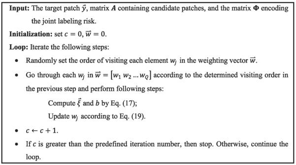
The optimization of weighting vector $\stackrel{\rightharpoonup }{w}$.

2.3.2. M-Step: Estimate the label fusion aresult $\stackrel{\rightharpoonup }{\eta }$

Given the estimated $\stackrel{\rightharpoonup }{w}$, the objective function to optimize $\stackrel{\rightharpoonup }{\eta }$ is given as:

$$\widehat{\stackrel{\rightharpoonup }{\eta }}=\text{arg}\underset{{\stackrel{\rightharpoonup }{l}}_{\in {[0,1]}^M}}{\max }p(\stackrel{\rightharpoonup }{\eta }=\stackrel{\rightharpoonup }{l}\mid \Lambda ,\widehat{\stackrel{\rightharpoonup }{w}}).$$ (20)

Here we follow the strategy of local weighted voting (Artaechevarria et al., 2009) to solve this problem by sequentially applying Eqs. (1) and (2). That is, given $\stackrel{\rightharpoonup }{\eta }$, we can refine the labeling dependency term Φ by Eqs. (8)–(10).

Fig. 1(c) shows the major differences between our joint label fusion and the conventional non-local based method. First, only a small number of closest patches are considered in label fusion in our method, as indicated by the fewer arrows in Fig. 1(c), compared with Fig. 1(b). Second, the dependency within each pair of candidate patches in labeling the target patch is considered, as shown by the dashed lines in Fig. 1(c). Third, the currently estimated label will feed back to the label fusion procedure to iteratively refine the labeling result, as designated by the two-end arrows in Fig. 1(c).

2.4. Discussions

2.4.1. Patch pre-selection

Pre-selecting patches in the search neighborhood n(u) is very important to speed up the procedure of label fusion and preclude the less similar candidate patches. In our implementation, we strictly follow the pre-selection procedure in (Coupe et al., 2011) by computing the structural similarity measurement ss:

$$\mathit{ss}(\stackrel{\rightharpoonup }{y},{\stackrel{\rightharpoonup }{a}}_j)=\frac{2{\mu }_y{\mu }_j}{{\mu }_y^2+{\mu }_j^2}\times \frac{2{\sigma }_y{\sigma }_j}{{\sigma }_y^2+{\sigma }_j^2},$$ (21)

where (μ_y, σ_y) and (μ_j, σ_j) are the mean and stand deviation of target patch $\stackrel{\rightharpoonup }{y}$ and candidate patch ${\stackrel{\rightharpoonup }{a}}_j$, respectively. In all experiments, we set the similarity threshold ε = 0.9 to discard the candidate patch ${\stackrel{\rightharpoonup }{a}}_j$ if $\mathit{SS}(\stackrel{\rightharpoonup }{y},{\stackrel{\rightharpoonup }{a}}_j)<\epsilon$.

2.4.2. Multipoint estimation

In the previous sections, we presented the label fusion method for labeling particular point u in the target image T. However, it is straightforward to obtain the labels for the whole patch ${\mathcal{P}}_T\left(u\right)$ by following the estimated weighting vector $\stackrel{\rightharpoonup }{w}$ at the target point u. As the result, each point has the multiple estimates from the neighboring points. Here, we use the majority voting strategy to fuse these multiple estimates after finishing the estimation at all points, in order to make the labeling result spatially smooth.

2.4.3. Generalization of our probability model

As mentioned early, most of the current patch-based label fusion method can be regarded as the simplified version of our probability model. For example, if we discard the correlation term in Eq. (14), the objective function turns to Eq. (7). Thus, our method simplifies to the sparse patch-based labeling method (Zhang et al., 2012a), which formulate the label fusion as the sparse representation problem with l₁-norm constraint. Certainly, more advanced priors such as elastic net (Tong et al., 2012), can be potentially incorporated in our probability model.

2.5. Summary

Given the registered atlas image I and associated label images L, our patch-based labeling method to label the target image T is summarized as follows:

1. Suppose the number of total iteration is H. Set h = 0.

2. Go through each point u ∈ Ω_T:

   • 2.1.
     Collect the candidate patches from all atlas images, constructing matrix A.
   • 2.2.
     Let r = 0.5 h/H (r is defined in Eq. (10)).
   • 2.3.
     Compute the matrix of joint labeling risk Φ in Eq. (14) based on the latest $\stackrel{\rightharpoonup }{\eta }$.
   • 2.4.
     Optimize the weighting vector $\stackrel{\rightharpoonup }{w}$ for the point u according to the optimization algorithm in Fig. 4.
   • 2.5.
     Predict the label $\stackrel{\rightharpoonup }{\eta }$ for point u by Eqs. (1) and (2).

3. h = h + 1.

4. If h < H, go to step 2. Otherwise, stop.

3. Experiments

In this section, we apply our patch-based labeling method on NIREP-NA40 and ADNI datasets to evaluate the labeling performance. For comparison, we also apply the conventional patch-based method by non-local weighting (Nonlocal-PBM) (Rousseau et al., 2011) and the recently proposed sparse patch-based labeling method (Sparse-PBM) (Zhang et al., 2012a) on the same dataset. Since our method utilizes the joint distribution of labeling consensus to guide the label fusion, we call our method Joint-PBM for short in the following. To quantitatively evaluate the labeling accuracy, we use the Dice ratio to measure the overlap degree between ROI O₁ and ROI O₂

$$\mathit{Dice}(O_1,O_2)=2\times \frac{\mid O_1\bigcap O_2\mid }{\mid O_1\mid +\mid O_2\mid },$$ (22)

where |·| means the volume of particular ROI.

3.1. Experiment result of hippocampus labeling on ADNI dataset

In many neuroscience studies, accurate delineation of hippocampus is very important for quantifying the convoluted inter-subject anatomical difference and subtle intra-subject longitudinal change, since the structural change of hippocampus is closely related with dementias, such as Alzheimer's disease (AD).

3.1.1. Data description

In this experiment, we randomly select 61 normal control (NC) subjects, 96 MCI (Mild Cognitive Impairment) subjects, and 41 AD subject from the ADNI dataset.¹ The detailed subject information is shown in Table 1. The following three pre-processing steps have been performed to all subject images: (1) Skull removal by a learning based meta-algorithm (Shi et al., 2012); (2) N4-based bias field correction (Tustison et al., 2010); (3) intensity standardization to normalize the intensity range (Madabhushi and Udupa, 2006). Semi-automated hippocampal volumetry was carried out using a commercial available high dimensional brain mapping tools (Medtronic Surgical Navigation Technologies, Louisville, CO), which has been validated and compared to manual tracing of the hippocampus (Hsu et al., 2002). In this experiment, we regard these hippocampal segmentations from ADNI as the ground truth.

Table 1.

Subject information of selected ADNI data in this experiment.

Group	No. of subjects	No. and percentage of males	Age, mean(SD)
NC	61	32 (52%)	73.7 (6.3)
MCI	96	43 (45%)	75.6 (7.2)
AD	41	22 (54%)	74.8 (8.0)

3.1.2. Experiment results

As it is common in the evaluation of label fusion method, we use the leave-one-out strategy to compare the labeling performance of Nonlocal-PBM, Sparse-PBM, and our proposed Joint-PBM methods. In each leave-one-out case, affine registration is first performed by FLIRT in the FSL toolbox (Smith et al., 2004) with 12 degrees of freedom and the default parameters (normalized mutual information similarity metric and search range ±20 in all directions). Then, we use diffeomorphic Demons (Vercauteren et al., 2009) for the deformable registration upon the affine registration result, also with the default registration parameters (smoothing sigma 1.8 and iterations in low, middle, and high resolution as 20 × 20 × 20).

The common parameters, such as patch size and search range, are widely discussed in (Coupe et al., 2011; Rousseau et al., 2011; Tong et al., 2012; Wang et al., 2012). Here, we fix the patch size as 7 × 7 × 7 and the search range 9 × 9 × 9 for all three label fusion methods. Specifically, we follow the patch pre-selection method and local adaptive selection of decay parameter (σ in Eq. (3)) in (Coupe et al., 2011) for Nonlocal-PBM. As reported in (Zhang et al., 2012a), we set the parameter for l₁ -norm strength as ρ=0.1 (Eq. (16)) for sparse-PBM. For our Joint-PBM method, the total number of iteration H in our Joint-PBM method is fixed to 5. Meanwhile, we set β=0.5 and ρ=0.1 throughout all the following experiments. Note, we will explain the way to determine the parameters β and ρ in our method after we show the overall labeling performance.

The overall Dice ratios on the left/right hippocampus by three label fusion results are shown in Table 2, where our Joint-PBM method has achieved 4.7% and 2.2% improvements over Nonlocal-PBM and Sparse-PBM, respectively, in terms of labeling accuracy. Specifically, we show the average and the standard deviation of Dice ratios in NC, MCI, and AD groups by three label fusion methods in Table 3. Again, our Joint-PBM method has the best labeling performance in each group. It is worth noting that the highest Dice ratio of hippocampus is 0.893 in (Wang et al., 2012), which is comparable with our Joint-PBM label fusion method. However, only 57 NC and 82 MCI subjects are evaluated in (Wang et al., 2012). As shown in Table 3, labeling the hippocampus of AD subjects are more challenging than MCI and NC groups. Discarding the AD subject, the overall overlap ratio of NC and MCI subjects by our method is able to reach 0.896.

Table 2.

The mean and the standard deviation of the Dice ratios on left and right hippocampi by Nonlocal-PBM (Coupe et al., 2011; Rousseau et al., 2011), Sparse-PBM (Zhang et al., 2012a), and our Joint-PBM.

Method	Left hippocampus	Right hippocampus	Overall
Nonlocal-PBM	0.854 ± 0.04	0.849 ± 0.043	0.852 ± 0.042
Sparse-PBM	0.877 ± 0.032	0.869 ± 0.036	0.873 ± 0.034
Joint-PBM	0.890 ± 0.022	0.884 ± 0.023	0.887 ± 0.022

Table 3.

The mean and the standard deviation of hippocampus Dice ratios in three groups (NC, MCI, and AD) by Nonlocal-PBM (Coupe et al., 2011; Rousseau et al., 2011), Sparse-PBM (Zhang et al., 2012a), and our Joint-PBM.

Method	NC	MCI	AD
Nonlocal-PBM	0.866 ± 0.034	0.859 ± 0.039	0.831 ± 0.046
Sparse-PBM	0.882 ± 0.030	0.873 ± 0.036	0.864 ± 0.041
Joint-PBM	0.899 ± 0.014	0.893 ± 0.019	0.870 ± 0.032

3.1.3. Discussions

In the following, we randomly select 15 different subjects from those 198 subjects as the test samples to examine each parameter/component in our label fusion method.

3.1.3.1. Parameter selection of ρ and β

Here, we will evaluate each parameter in Joint-PBM method, in order to acquire the optimal parameter set. The ranges of β and ρ are (0.1~1.0) and (0.01–0.25), respectively. The Dice ratios w.r.t. β and ρ are shown in Fig. 5, where β=0.5 and ρ=0.1 achieve the highest Dice ratios in our joint label fusion method. Thus, we fix β = 0.5 and ρ = 0.1 throughout the experiments.

Fig. 5.

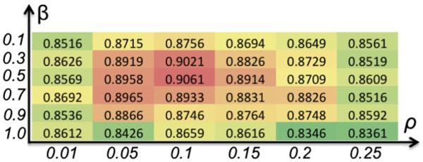
The demonstration of determining optimal parameters β and ρ in our method.

3.1.3.2. The role of dependency term Φ

Next, we specifically evaluate the role of two terms in modeling dependency, i.e., ${\varphi }_{\mathit{ij}}^{\mathrm{A}}$ and ${\varphi }_{\mathit{ij}}^{\Lambda }$ in our method. Fig. 6 shows the evolution curves of average Dice ratios by 198 subjects as the number of iteration increases. As the baseline method, we also plot the average Dice ratio by Sparse-PBM as a blue straight line in the figure. In the beginning of our joint label fusion, only the term ${\varphi }_{\mathit{ij}}^{\mathrm{A}}$ contributes to the modeling of the dependency among candidate patches. Compared with Sparse-PBM which lacks of the dependency modeling, its average Dice ratio is 1% lower than our Joint-PBM method in the first iteration. After obtaining the initial estimation of labeling result, our Joint-PBM method is able to update the dependency probability by further inspecting whether two candidate patches achieve labeling consensus towards the latest label fusion results. As shown by the red curve in Fig. 6, the Dice ratios increase to 0.887, indicating the effectiveness of ${\varphi }_{\mathit{ij}}^{\Lambda }$ in correcting possible mislabeling.

Fig. 6.

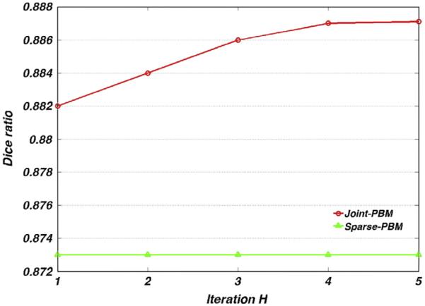
The evolution curves of Dice ratio by Sparse-PBM (green) and our Joint-PBM (red) methods, respectively.

3.1.3.3. The influence of the number of atlases

Here, we evaluate the evolution curves w.r.t. the atlas number in Fig. 7 by Nonlocal-PBM (red), Sparse-PBM (green), and Joint-PBM (red), respectively. It is clear that (1) the Dice ratios keep increasing for all three label fusion methods, as more and more atlases are included; and (2) our Joint-PBM method consistently achieves the highest Dice ratios in all cases.

Fig. 7.

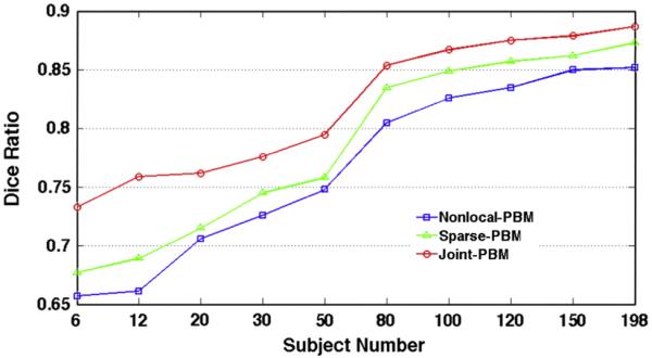
The evolution curves of Dice ratio w.r.t. the number of atlases used by Nonlocal-PBM (blue), Sparse-PBM (green), and Joint-BPM (red), respectively.

3.1.3.4. The influence of patch size and search range

Given the optimized parameters, we examine the influences of patch size and search range in Nonlocal-PBM, Sparse-PBM, and our Joint-PBM methods. Specifically, we perform these three label fusion methods with patch size from 3 × 3 × 3 to 11 × 11 × 11 and search range from 5 × 5 ×5 to 13 × 13 × 13. The Dice ratios w.r.t. different patch size and search range are shown in Fig. 8(a) and (b), with blue, green, and red curves representing the results by the Nonlocal-PBM, sparse-PBM, and our Joint-PBM methods, respectively.

Fig. 8.

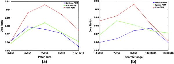
The evolution curves of Dice ratio by the three label fusion methods, with respective to patch size (a) and search range (b).

3.1.3.5. The influence of patch pre-selection

Patch pre-selection is able to not only speed up the label fusion procedure, but also improve the robustness of label fusion by excluding the unrelated patches. To demonstrate this point, we evaluate the label fusion accuracy when applying different thresholds in pre-selection (ss in Eq. (21)). Fig. 9 shows the evolution curve of Dice ratio by Nonlocal-PBM (blue curve), Sparse-PBM (green curve), and Joint-PBM (red curve), where the threshold degree ε for pre-selection ranges from 0.60 to 0.95. It is apparent that, for three label fusion methods, the Dice ratios keep increasing as the threshold increases, indicating the importance of pre-selection procedure in label fusion. Although pre-selection can help improve the robustness of label fusion, if pre-selection criteria are too strict (i.e., ε > 0.85 in Non-local PBM and ε > 0.90 in both Sparse and Joint-PBM), the label fusion accuracy could be decreased as shown in the right part of Fig. 9, since too strict pre-selection criteria could exclude the image patches with correct label.

Fig. 9.

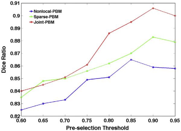
The evolution curve of Dice ratio w.r.t. the pre-selection threshold ε by three label fusion methods.

3.2. Experiment result of whole brain labeling on NIREP-NA40 dataset

3.2.1. Data description

The NIREP dataset consists of 16 MR images of 8 normal male adults and 8 normal female adults, each with 32 manually delineated gray matter ROIs. All 16 MR images have been aligned according to the anterior and posterior commissures (AC and PC). The image size is 256 × 300 × 256, and the voxel dimension is 0.7 × 0.7 × 0.7 mm³. The following pre-processing steps have been applied on these NA40 dataset: (1) N4-based bias correction (Tustison et al., 2010); and (2) intensity standardization (Madabhushi and Udupa, 2006).

3.2.2. Experiment results

Leave-one-out strategy is used in this experiment by alternatively taking one of the 16 NA40 images as the target image. For each leave-one-out case, affine and deformable registrations are sequentially deployed by FLIRT and Diffeomorphic Demons with the same registration parameters in labeling hippocampus. Since we have determined the optimal parameters in Section 3.1, here, we use these parameters in labeling 32 ROIs in NA40 dataset, i.e., patch size is 7 × 7 × 7 and search range is 9 × 9 × 9. Our Joint-PBM takes 5 iterations with ρ = 0.1 and β = 0.5.

Table 4 displays the averaged Dice ratio in each brain structure (left and right combined) upon 16 leave-one-out cases. From second to the last column, we show the average Dice ratios by Nonlocal-PBM, Sparse-PBM, and our Joint-PBM, respectively. The overall Dice ratios across 32 ROIs are 0.792 by Nonlocal-PBM, 0.803 by Sparse-PBM, and 0.827 by Joint-PBM. It is clear that our Joint-PBM method achieves the best labeling accuracy over the other two methods. It is worth noting that the overall Dice ratio was reported as 0.823 by a non-local label fusion method in (Rousseau et al., 2011), which is comparable with our method. However, they used SyN (Avants et al., 2008) as the deformable registration method before patch-based labeling and also STAPLE (Warfield et al., 2004) as the post-processing step to fuse the multiple estimates, where computational costs of both steps are very expensive.

Table 4.

The average Dice ratios of 32 ROIs in NIREP-NA40 dataset by Nonlocal-PBM, Sparse-PBM, and Joint-PBM.

ROI	Nonlocal-PBM	Sparse-PBM	Joint-PBM
Left occipital lobe	0.801 ± 0.018	0.815 ± 0.019	0.833 ± 0.011
Right occipital lobe	0.813 ± 0.016	0.820 ± 0.016	0.859 ± 0.009
Left cingulate gyrus	0.815 ± 0.024	0.811 ± 0.020	0.819 ± 0.016
Right cingulate gyrus	0.812 ± 0.022	0.814 ± 0.016	0.852 ± 0.014
Left insula gyrus	0.851 ± 0.019	0.855 ± 0.016	0.862 ± 0.014
Right insula gyrus	0.873 ± 0.020	0.878 ± 0.029	0.890 ± 0.019
Left temporal pole	0.837 ± 0.015	0.838 ± 0.015	0.842 ± 0.014
Right temporal pole	0.829 ± 0.015	0.841 ± 0.016	0.875 ± 0.017
Left superior temporal gyrus	0.779 ± 0.024	0.781 ± 0.019	0.801 ± 0.016
Right superior temporal gyrus	0.777 ± 0.011	0.784 ± 0.015	0.811 ± 0.010
Left infero temporal region	0.832 ± 0.012	0.848 ± 0.012	0.867 ± 0.011
Right infero temporal region	0.833 ± 0.023	0.832 ± 0.015	0.871 ± 0.016
Left parahippocampal gyrus	0.829 ± 0.015	0.831 ± 0.011	0.842 ± 0.017
Rgiht parahippocampal gyrus	0.843 ± 0.018	0.851 ± 0.014	0.864 ± 0.009
Left frontal pole	0.820 ± 0.016	0.824 ± 0.012	0.849 ± 0.011
Right frontal pole	0.804 ± 0.017	0.821 ± 0.015	0.852 ± 0.011
Left superior frontal gyrus	0.807 ± 0.021	0.805 ± 0.013	0.822 ± 0.015
Right superior frontal gyrus	0.785 ± 0.023	0.800 ± 0.020	0.837 ± 0.017
Left middle frontal gyrus	0.791 ± 0.022	0.809 ± 0.017	0.819 ± 0.018
Right middle frontal gyrus	0.753 ± 0.015	0.763 ± 0.016	0.805 ± 0.015
Left inferior gyrus	0.755 ± 0.013	0.758 ± 0.011	0.785 ± 0.012
Right inferior gyrus	0.751 ± 0.017	0.775 ± 0.015	0.790 ± 0.011
Left orbital frontal gyrus	0.833 ± 0.012	0.841 ± 0.012	0.863 ± 0.008
Right orbital frontal gyrus	0.831 ± 0.008	0.835 ± 0.010	0.860 ± 0.009
Left precentral gyrus	0.762 ± 0.019	0.785 ± 0.014	0.801 ± 0.015
Right precentral gyrus	0.744 ± 0.021	0.762 ± 0.015	0.789 ± 0.014
Left superior parietal lobule	0.742 ± 0.023	0.756 ± 0.015	0.802 ± 0.011
Right superior parietal lobule	0.739 ± 0.017	0.780 ± 0.013	0.805 ± 0.010
Left inferior parietal lobule	0.759 ± 0.024	0.771 ± 0.017	0.800 ± 0.017
Right inferior parietal lobule	0.738 ± 0.025	0.802 ± 0.018	0.812 ± 0.019
Left postcentral gyrus	0.707 ± 0.026	0.713 ± 0.021	0.756 ± 0.022
Right postcentral gyrus	0.694 ± 0.022	0.711 ± 0.021	0.738 ± 0.020

3.2.3. Discussions

3.2.3.1. The influence of deformable registration

Specifically, we evaluate the effect of deformable registration in patch-based labeling method. As we all know, there are two terms in the energy function of deformable registration, i.e., data fitting term and the regularization term. Generally, the fitting term aims to maximize the similarity between two images, and the regularization term makes the deformation field as smooth as possible. In patch-based label fusion method, it is desirable to deform the atlas images as similar as possible to the target image by deformable image registration. However, we argue that over-registration, which makes two images unreasonably similar but at the cost of very aggressive deformation field, will undermine the label fusion result since the over-registration might tear down the inherent topology of anatomical structure.

To demonstrate this point, we examine the evolution of Dice ratio with changes of parameters in deformable image registration. In general, the number of iterations and the size of the smoothing kernel are the two important parameters in the diffeomorphic Demons, for controling the smoothness of deformation field. In Fig. 10, the horizontal and vertical axes denote the sigma for deformation smoothing and the iteration number, respectively, where the larger number of iterations and the smaller degree of sigma lead to more aggressive registration result. Taking precentral gyrus as example, we show the Dice ratios w.r.t. different parameters in diffeomorphic Demons in Fig. 10. It is interesting to see that (1) the Dice ratio first increases as the registration becomes more and more accurate; and then (2) the Dice ratio decreases when the registration is too aggressive to preserve the topology of anatomical structures after warping the atlas image to the target image space.

Fig. 10.

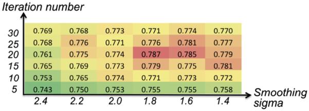
The evolution of Dice ratio w.r.t. the aggressiveness of deformable image registration.

3.2.3.2. The convergence of our Joint-PBM method

Since our Joint-PBM method falls into the EM framework, we specifically evaluate the convergence of our label fusion method. Fig. 11 shows the evolution of Dice ratio during joint label fusion, where each curve denotes the average Dice ratio of 32 ROIs at different stages of one leave-one-out case. It is clear that the Dice ratio keeps increasing in the first half of the whole label fusion procedure and then quickly converges, which demonstrates the robustness of our iterative label fusion method.

Fig. 11.

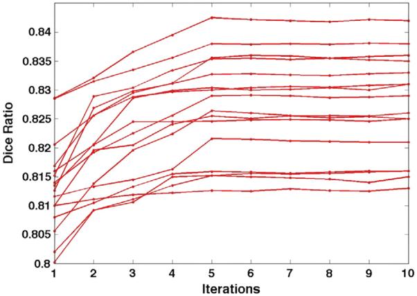
The evolution curves of Dice ratio at different stages of Joint-PBM method, where each curve denotes the evolution of Dice ratio in a leave-out-out case.

3.3. Computation time

3.3.1. Computational complexity

Suppose there are Q candidate patches in labeling a particular point, where the length of each patch is P. Then the sizes of matrix A and Φ are P × Q and Q × Q, respectively. For classic LASSO problem (with the objective function shown in Eq. (7)), the computational complexity is $\mathcal{O}(P\times Q\times \min (P,Q\left)\right)$ (Efron et al., 2004). With the quadratic term Φ in our energy function (Eq. (14)), the computation cost of our Joint-PBM method increases to $\mathcal{O}(P\times Q\times \min (P,Q)+Q^2)$.

In the multi-atlas labeling scenario, the number of candidate patches is usually much larger than the length of patch, i.e., Q ⪢ P. Thus, the computational complexities of Sparse-PBM and our Joint-PBM are approximately $\mathcal{O}\left(P^2\right)$ and $\mathcal{O}\left(Q^2\right)$, respectively.

3.3.2. Experiment result

All the experiments are performed on our DELL computation server with 2 CPUs (each with four 2.0 GHz cores) and 32G memory. We utilize the OpenMP technique² to parallelize the labeling procedure independently for each point. The computation time of each step in labeling one image from NIREP-NA40 dataset, with other 15 images as the atlases, is shown in Table 5. In general, our Joint-PBM takes 7.7 h to labeling the whole brain with 32 ROIs. It is worth noting that the computational times for labeling hippocampus by three labeling methods are comparable, i.e., 15 min by Nonlocal-PBM, 19 min by Sparse-PBM, and 21 min by Joint-PBM, since the volume of hippocampus is often small (~5000 voxels).

Table 5.

The computation time (unit: minute) on NIREP dataset by Nonlocal-PBM, Sparse-PBM, and Joint-PBM.

Steps	Nonlocal-PBM	Sparse-PBM	Joint-PBM
Affine registration	20	20	20
Deformable registration	30	30	30
Patch-based labeling	50	150	410
Overall	100	200	460

4. Conclusion

In this paper, we present a novel probability model for multi-atlas label fusion. In general, we estimate the optimal weights for label fusion by seeking for not only the best representation but also the largest unanimity in labeling accuracy. To achieve it, sparsity is used as the prior on weighting vectors to suppress the contribution from ambiguous patches. Different from other conventional patching labeling methods, we explicitly model the labeling dependency of the entire candidate patches for achieving the highest labeling accuracy simultaneously. We further describe the label fusion procedure as the generative probability model, where the label fusion results are iteratively refined in the EM framework. Our joint label fusion method achieves better performance than conventional methods in terms of labeling accuracy and robustness, indicating its potential for future clinical applications.

References

- Artaechevarria X, Munoz-Barrutia A, Ortiz-de-Solorzano C. Combination strategies in multi-atlas image segmentation: application to brain MR data. IEEE Transactions on Medical Imaging. 2009;28:1266–1277. doi: 10.1109/TMI.2009.2014372. [DOI] [PubMed] [Google Scholar]
- Avants BB, Epstein CL, Grossman M, Gee JC. Symmetric diffeomorphic image registration with cross-correlation: evaluating automated labeling of elderly and neurodegenerative brain. Medical Image Analysis. 2008;12:26–41. doi: 10.1016/j.media.2007.06.004. [DOI] [PMC free article] [PubMed] [Google Scholar]
- Awate SP, Whitaker RT. Unsupervised, information-theoretic, adaptive image filtering for image restoration. IEEE Transactions on Pattern Analysis and Machine Intelligence. 2006;28:364–376. doi: 10.1109/TPAMI.2006.64. [DOI] [PubMed] [Google Scholar]
- Buades A, Coll B, Morel JM. A review of image denoising algorithms, with a new one. Multiscale Modeling and Simulation. 2005;4:490–530. [Google Scholar]
- Christensen G, Geng X, Kuhl J, Bruss J, Grabowski T, Pirwani I, Vannier M, Allen J, Damasio H. Biomedical Image Registration. 2006. Introduction to the non-rigid Image registration evaluation project (NIREP) pp. 128–135. [Google Scholar]
- Coupe P, Manjon JV, Fonov V, Pruessner J, Robles M, Collins DL. Patch-based segmentation using expert priors: application to hippocampus and ventricle segmentation. NeuroImage. 2011;54:940–954. doi: 10.1016/j.neuroimage.2010.09.018. [DOI] [PubMed] [Google Scholar]
- Devanand D, Pradhaban G, Liu X, Khandji A, De Santi S, Segal S, Rusinek H, Pelton G, Honig L, Mayeux R, Stern Y, Tabert M, de Leon M. Hippocampal and entorhinal atrophy in mild cognitive impairment: prediction of Alzheimer disease. Neurology. 2007;68:828–836. doi: 10.1212/01.wnl.0000256697.20968.d7. [DOI] [PubMed] [Google Scholar]
- Dickerson BC, Goncharova I, Sullivan MP, Forchetti C, Wilson RS, Bennett DA, Beckett LA, deToledo-Morrell L. MRI-derived entorhinal and hippocampal atrophy in incipient and very mild Alzheimer's disease. Neurobiology of Aging. 2001;22:747–754. doi: 10.1016/s0197-4580(01)00271-8. [DOI] [PubMed] [Google Scholar]
- Efron B, Hastie T, Johnstone I, Tibshirani R. Least angle regression. Annals of Statistics. 2004;32:407–499. [Google Scholar]
- Fennema-Notestine C, Hagler DJ, McEvoy LK, Fleisher AS, Wu EH, Karow DS, Dale AM. Structural MRI biomarkers for preclinical and mild Alzheimer's disease. Human Brain Mapping. 2009;30:3238–3253. doi: 10.1002/hbm.20744. [DOI] [PMC free article] [PubMed] [Google Scholar]
- Holland D, Desikan RS, Dale AM, McEvoy LK, Alzheimer’s Disease Neuroimaging, I Rates of Decline in Alzheimer Disease Decrease with Age. PLoS ONE. 2012;7:e42325. doi: 10.1371/journal.pone.0042325. [DOI] [PMC free article] [PubMed] [Google Scholar]
- Hsu Y-Y, Schuff N, Du A-T, Mark K, Zhu X, Hardin D, Weiner MW. Comparison of automated and manual MRI volumetry of hippocampus in normal aging and dementia. Journal of Magnetic Resonance Imaging. 2002;16:305–310. doi: 10.1002/jmri.10163. [DOI] [PMC free article] [PubMed] [Google Scholar]
- Koller D, Friedman N. Probabilistic Graphical Models. MIT Press; Massachusetts: 2009. [Google Scholar]
- Madabhushi A, Udupa J. New methods of MR image intensity standardization via generalized scale. Medical Physics. 2006;33:3426–3434. doi: 10.1118/1.2335487. [DOI] [PubMed] [Google Scholar]
- Manjón JV, Coupé P, Martí-Bonmatí L, Collins DL, Robles M. Adaptive non-local means denoising of MR images with spatially varying noise levels. Journal of Magnetic Resonance Imaging. 2011;31:192–203. doi: 10.1002/jmri.22003. [DOI] [PubMed] [Google Scholar]
- Paus TÅ, Zijdenbos A, Worsley K, Collins DL, Blumenthal J, Giedd JN, Rapoport JL, Evans AC. Structural maturation of neural pathways in children and adolescents: in vivo study. Science. 1999:1908–1911. doi: 10.1126/science.283.5409.1908. [DOI] [PubMed] [Google Scholar]
- Protter M, Elad M, Takeda H, Milanfar P. Generalizing the nonlocal-means to super-resolution reconstruction. IEEE Transactions on Medical Imaging. 2009;18:36–51. doi: 10.1109/TIP.2008.2008067. [DOI] [PubMed] [Google Scholar]
- Rousseau F, Habas PA, Studholme C. A supervised patch-based approach for human brain labeling. IEEE Transactions on Medical Imaging. 2011;30:1852–1862. doi: 10.1109/TMI.2011.2156806. [DOI] [PMC free article] [PubMed] [Google Scholar]
- Seeger Matthias, Gerwinn Sebastian, Bethge Matthias. Bayesian inference for sparse generalized linear models. Europe Conference on Machine Learning.2007. [Google Scholar]
- Seeger MW. Bayesian inference and optimal design for the sparse linear model. Journal of Machine Learning Research. 2008;9:759–813. [Google Scholar]
- Shi F, Wang L, Dai Y, Gilmore J, Lin W, Shen D. LABEL: Pediatric brain extraction using learning-based meta-algorithm. NeuroImage. 2012;62:1975–1986. doi: 10.1016/j.neuroimage.2012.05.042. [DOI] [PMC free article] [PubMed] [Google Scholar]
- Smith SM, Jenkinson M, Woolrich MW, Beckmann CF, Behrens TEJ, Johansen-Berg H, Bannister PR, De Luca M, Drobnjak I, Flitney DE, Niazy RK, Saunders J, Vickers J, Zhang Y, De Stefano N, Brady JM, Matthews PM. Advances in functional and structural MR image analysis and implementation as FSL. NeuroImage. 2004;23:S208–S219. doi: 10.1016/j.neuroimage.2004.07.051. [DOI] [PubMed] [Google Scholar]
- Tibshirani R. Regression shrinkage and selection via the lasso. Journal of the Royal Statistical Society: Series B (Statistical Methodology) 1996;58:267–288. [Google Scholar]
- Tong T, Wolz R, Hajnal JV, Rueckert D. Segmentation of Brain Images via Sparse Patch Representaion. MICCAI Workshop on Sparsity Techniques in Medical Imaging; Nice, France. 2012. [Google Scholar]
- Tustison N, Avants B, Cook P, Zheng Y, Egan A, Yushkevich P, Gee J. N4ITK: Improved N3 Bias Correction. IEEE Transactions on Medical Imaging. 2010;29:1310–1320. doi: 10.1109/TMI.2010.2046908. [DOI] [PMC free article] [PubMed] [Google Scholar]
- Vercauteren T, Pennec X, Perchant A, Ayache N. Symmetric log-domain diffeomorphic registration: a demons-based approach. Medical Image Computing and Computer-Assisted Intervention-MICCAI. 2008;2008:754–761. doi: 10.1007/978-3-540-85988-8_90. [DOI] [PubMed] [Google Scholar]
- Vercauteren T, Pennec X, Perchant A, Ayache N. Diffeomorphic demons: efficient non-parametric image registration. NeuroImage. 2009;45:S61–S72. doi: 10.1016/j.neuroimage.2008.10.040. [DOI] [PubMed] [Google Scholar]
- Vinje WE, Gallant JL. Sparse coding and decorrelation in primary visual cortex during natural vision. Science. 2000;287:1273–1276. doi: 10.1126/science.287.5456.1273. [DOI] [PubMed] [Google Scholar]
- Wang H, Suh JW, Das SR, Craige C, Yushkevich PA. Multi-atlas segmentation with joint label fusion. IEEE Transactions on Pattern Analysis and Machine Intelligence. 2013;35:611–623. doi: 10.1109/TPAMI.2012.143. [DOI] [PMC free article] [PubMed] [Google Scholar]
- Wang H, Suh JW, Pluta J, Altinay M, Yushkevich P. CVPR 2011. 2011. Regression-Based Label Fusion for Multi-Atlas Segmentation. [DOI] [PMC free article] [PubMed] [Google Scholar]
- Warfield SK, Zou KH, Wells WM. Simultaneous truth and performance level estimation (STAPLE): an algorithm for the validation of image segmentation. IEEE Transactions on Medical Imaging. 2004;23:903–921. doi: 10.1109/TMI.2004.828354. [DOI] [PMC free article] [PubMed] [Google Scholar]
- Westerhausen R, Luders E, Specht K, Ofte SH, Toga AW, Thompson PM, Helland T, Hugdahl K. Structural and Functional Reorganization of the Corpus Callosum between the Age of 6 and 8 Years. 2011. pp. 1012–1017. [DOI] [PMC free article] [PubMed] [Google Scholar]
- Wu G, Kim M, Wang Q, Shen D. S-HAMMER: Hierarchical Attribute-Guided, Symmetric Diffeomorphic Registration for MR Brain Images. Human Brain Mapping. 2013 doi: 10.1002/hbm.22233. [DOI] [PMC free article] [PubMed] [Google Scholar]
- Wu G, Qi F, Shen D. Information Processing in Medical Imaging. 2007. Learning best features and deformation statistics for hierarchical registration of MR brain images; pp. 160–171. [DOI] [PubMed] [Google Scholar]
- Wu G, Wang Q, Jia H, Shen D. Feature-based groupwise registration by hierarchical anatomical correspondence detection. Human Brain Mapping. 2012a;33:253–271. doi: 10.1002/hbm.21209. [DOI] [PMC free article] [PubMed] [Google Scholar]
- Wu G, Wang Q, Zhang D, Shen D. Robust Patch-Based Multi-Atlas Labeling by Joint Sparsity Regularization. MICCAI Workshop on Sparsity Techniques in Medical Imaging; Nice, France. 2012b. [Google Scholar]
- Wu G, Yap P-T, Kim M, Shen D. TPS-HAMMER: Improving HAMMER registration algorithm by soft correspondence matching and thin-plate splines based deformation interpolation. NeuroImage. 2010;49:2225–2233. doi: 10.1016/j.neuroimage.2009.10.065. [DOI] [PMC free article] [PubMed] [Google Scholar]
- Wu TT, Lange K. Coordinate descent algorithms for lasso penalized regression. The Annals of Applied Statistics. 2008;2:224–244. doi: 10.1214/10-AOAS388. [DOI] [PMC free article] [PubMed] [Google Scholar]
- Yan Z, Zhang S, Liu X, Metaxas D, Montillo A. ISBI 2013. 2013. Accurate Segmentation of Brain Images into 34 Structures Combining a Non-stationary Adaptive Statistical Atlas and a Multi-atlas with Applications to Alzheimer's disease. [DOI] [PMC free article] [PubMed] [Google Scholar]
- Zhang D, Guo Q, Wu G, Shen D. Sparse Patch-Based Label Fusion for Multi-Atlas Segmentation, MBIA; Nice, France. 2012a. [Google Scholar]
- Zhang S, Zhan Y, Dewan M, Huang J, Metaxas DN, Zhou XS. Towards robust and effective shape modeling: sparse shape composition. Medical Image Analysis. 2012b;16:265–277. doi: 10.1016/j.media.2011.08.004. [DOI] [PubMed] [Google Scholar]
- Zhang S, Zhan Y, Metaxas D. Deformable segmentation via sparse representation and dictionary learning. Medical Image Analysis. 2012c;16:1385–1396. doi: 10.1016/j.media.2012.07.007. [DOI] [PubMed] [Google Scholar]