Neural portraits of perception: Reconstructing face images from evoked brain activity

Abstract

Recent neuroimaging advances have allowed visual experience to be reconstructed from patterns of brain activity. While neural reconstructions have ranged in complexity, they have relied almost exclusively on retinotopic mappings between visual input and activity in early visual cortex. However, subjective perceptual information is tied more closely to higher-level cortical regions that have not yet been used as the primary basis for neural reconstructions. Furthermore, no reconstruction studies to date have reported reconstructions of face images, which activate a highly distributed cortical network. Thus, we investigated (a) whether individual face images could be accurately reconstructed from distributed patterns of neural activity, and (b) whether this could be achieved even when excluding activity within occipital cortex. Our approach involved four steps. (1) Principal component analysis (PCA) was used to identify components that efficiently represented a set of training faces. (2) The identified components were then mapped, using a machine learning algorithm, to fMRI activity collected during viewing of the training faces. (3) Based on activity elicited by a new set of test faces, the algorithm predicted associated component scores. (4) Finally, these scores were transformed into reconstructed images. Using both objective and subjective validation measures, we show that our methods yield strikingly accurate neural reconstructions of faces even when excluding occipital cortex. This methodology not only represents a novel and promising approach for investigating face perception, but also suggests avenues for reconstructing ‘offline’ visual experiences—including dreams, memories, and imagination—which are chiefly represented in higher-level cortical areas.

INTRODUCTION

Neuroimaging methods such as fMRI have provided tremendous insight into how distinct brain regions contribute to processing different kinds of visual information (e.g, colors, orientations, shapes, or higher-level visual categories such as faces or scenes). These studies have supported inferences about the neural mechanisms or computations that underlie visual perception by documenting how various types of stimuli influence brain activity. However, knowledge about the relationship between visual input and corresponding neural activity can also be used for reverse inference: to predict or literally reconstruct a visual stimulus based on observed patterns of neural activity. That is, by understanding how an individual’s brain represents visual information, it is possible to ‘see’ what someone else sees. While there are a relatively limited number of studies reporting neural reconstructions to date, the feats of reconstruction that have been achieved thus far are impressive. In addition to reconstruction of lower-order information such as binary contrast patterns (Miyawaki et al., 2008; Thirion et al., 2006) and colors (Brouwer and Heeger, 2009), there are also examples of successful reconstruction of handwritten characters (Schoenmakers et al., 2013), natural images (Naselaris et al., 2009), and even complex movie clips (Nishimoto et al., 2011).

However, even reconstructions of complex visual information have relied almost exclusively on exploiting information represented in early visual cortical regions (typically V1 and V2). Exceptions to this include evidence from Brouwer and Heeger (2009) that color can be reconstructed from responses in intermediate visual areas such as V4, and evidence from Naselaris et al. (2009) showing that reconstruction of natural images benefits from inclusion of higher-level visual areas (anterior occipital cortex) that are thought to represent semantic information about images. But reconstructions of visual stimuli based on patterns of activity outside occipital cortex have not, to our knowledge, been reported. The potential for reconstructions from higher-level regions (e.g., ventral temporal cortex or even fronto-parietal cortex) is enticing because reconstructions from these regions may be more closely related to perceptual experience as opposed to visual analysis (Smith et al., 2012).

Here, we attempted to reconstruct images of faces— a stimulus class that has not previously been reconstructed from neural activity. While face images—like other visual images—could, in theory, be reconstructed from patterns of activity in early visual cortex (i.e., via representations of contrast, orientation, etc.), we were also interested in the potential to reconstruct faces based on patterns of activity in higher-level regions. A number of face-selective (or face-preferring) regions have been identified outside of early visual cortex—for example, the occipital face area (Gauthier et al., 2000), fusiform face area (Kanwisher et al., 1997), and superior temporal sulcus (Puce et al., 1998) are all thought to contribute to aspects of face perception. Furthermore, other non-occipital regions have been implicated in the processing of relatively subjective face properties such as race (Hart et al., 2000) and emotional expression (Whalen et al., 1998). Thus, faces represent a class of visual stimuli that may be particularly suitable for ‘higher-level’ neural reconstructions. Moreover, a major computational advantage of using face stimuli is that there are previously established methods, based on principal components analysis (PCA), to dramatically reduce the dimensionality of face images such that an individual face can be accurately represented by a relatively small number of components. The representation of faces via a limited set of PCA components (or eigenfaces) has proved useful in domains such as face recognition (Turk and Pentland, 1991), but the application to neural reconstructions is novel.

In short, our approach to reconstructing face images from brain activity involved four basic steps (Fig. 1). First, PCA was applied to a large set of training faces to identify a set of components (eigenfaces) that efficiently represented the face images in a relatively low dimensional space (note: this step was based on the faces images themselves and was entirely unrelated to neural activity). Second, a machine-learning algorithm (partial least squares regression, or PLSR) was used to map patterns of fMRI activity (recorded as participants viewed faces) to individual eigenfaces (i.e., the PCA components representing the face images). Third, based on patterns of neural activity elicited by a distinct set of faces (test faces), the PLSR algorithm predicted the associated eigenface component scores. Fourth, an inverse transformation was applied to the component scores that were predicted for each test face to generate a reconstruction of that face. To empirically validate the success of neural reconstructions, and to compare reconstructions across distinct brain regions, we assessed whether reconstructed faces could be identified as corresponding to the original (target) image. Identification accuracy was assessed via objective, computer-based measures of image similarity and via subjective, human-based reports of similarity.

Figure 1.

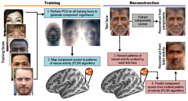
Overview of reconstruction method. First, principal component analysis (PCA) was applied to a set of 300 training faces to generate component eigenfaces. Second, component scores from the training faces were mapped to evoked patterns of neural activity using a partial least squares regression (PLSR) algorithm. Third, based on patterns of activity elicited during the viewing of a distinct set of 30 test faces, the PLSR algorithm predicted each component score for each test face. Fourth, predicted component scores were used to reconstruct the viewed face. For comparison, test faces were also directly reconstructed based on component scores extracted from the test face (a ‘non-neural reconstruction’; grey box; see also Fig. S1).

METHODS

Participants

Six participants (2 female) between the ages of 18 and 35 (mean age = 21.7) were recruited from the Yale University community. Informed consent was obtained in accordance with the Yale University Institutional Review Board. Participants received payment in exchange for their participation.

Materials

A total of 330 face images were used in the study. Face images were obtained from a variety of online sources [e.g., www.google.com/images, www.cs.mass.edu/lfw (Huang and Learned-Miller, 2007)] and were selected such that faces were generally forward facing with eyes and mouth visible in each image. The faces varied in terms of race, gender, expression, hair, etc. For all images, the location of the left eye, right eye, and mouth were first manually labeled (in x/y coordinates). Each image was then cropped and resized to 110 by 154 pixels with the constraints that (a) the mean vertical position of the eyes was 52 pixels above the vertical position of the mouth, (b) the image was 110 pixels wide, centered about the mean of the horizontal position of the mouth and the center point of the eyes, (c) 61 pixels were included above the mean vertical position of the eyes, and (d) 41 pixels were included below the vertical position of the mouth. Thus, all 330 face images were of equal size and the centers of the eyes and mouth of each face were carefully aligned to one another—criteria that were found to yield highly effective image registration in studies of computerized face image classification (Donato et al., 1999).

300 of the 330 face images were designated as training faces and the remaining 30 faces were reserved as test faces. The 30 test faces were held constant across participants and were pseudo-randomly selected such that they included a range of ethnicities, genders, and expressions.

Procedure

During each trial in the experiment, a face image was presented (2000 ms) and participants indicated via button box whether they had seen that face on any of the preceding trials (left key = ‘new’, right key = ‘old’). Each face image was followed by a 1300 ms fixation cross and then a distracting “arrow task” (5200 ms) that required participants to indicate, via button press, the directionality of four left- or right-facing arrows. The purpose of the arrow task was dually to keep subjects alert and to attenuate the rehearsal of images in visual short-term memory. Finally, another fixation cross was presented (1500 ms) before the start of the next trial.

There were a total of 360 trials in the experiment: 300 training image trials and 60 test image trials. Each training image appeared once and each test image appeared twice. The test image trials were pseudorandomly intermixed with the training image trials such that the first and second presentations of each test image appeared within the same run and were not adjacent to one another.

fMRI Methods

fMRI scanning was conducted at the Yale Magnetic Resonance Research Center (MRRC) on a 3.0 T MRI scanner. Following a high resolution (1.0 × 1.0 × 1.0 mm) anatomical scan and a coplanar (1.0 × 1.0 × 4.0 mm) anatomical scan, functional images were obtained using a T2*-weighted 2D gradient echo sequence with a repetition time (TR) of 2s, an echo time (TE) of 25 ms, and a flip angle of 90°, producing 34 slices at a resolution of 3.0 × 3.0 × 4.0 mm. The functional scan was divided into six runs, each consisting of 305 volumes. The first 5 volumes of each run were discarded. Thus, each run consisted of 60 trials, with 5 volumes per trial and 2 seconds per volume. fMRI data preprocessing was conducted using SPM8 (Wellcome Department of Cognitive Neurology, London). Images were first corrected for slice timing and head motion. High-resolution anatomical images were co-registered to the functional images and segmented into gray matter, white matter, and cerebrospinal fluid. Segmented gray matter images were ‘skull-stripped’ and normalized to a gray matter Montreal Neurological Institute (MNI) template. Resulting parameters were used for normalization of functional images. Functional images were resampled to 3-mm cubic voxels. fMRI data were analyzed using a general linear model (GLM) in which a separate regressor was included for each trial. Trials were modeled using a canonical hemodynamic response function and its first-order temporal derivative. Additional regressors representing motion and scan number were also included. Trial-specific beta values for each voxel were used as representations of brain activity in all further analyses.

Region-of-interest (ROI) masks were generated using the Anatomical Automatic Labeling atlas (http://www.cyceron.fr/web/aal__anatomical_automatic_labeling.html). Masks were generated representing occipital cortex, fusiform gyrus, lateral temporal cortex, hippocampus, amygdala, lateral parietal cortex, medial parietal cortex, lateral prefrontal cortex and medial prefrontal cortex. The masks ranged in size from 194 voxels (amygdala) to 10,443 voxels (lateral prefrontal). All reported analyses of individual regions (or fusiform combined with occipital) were based either on the 1500 voxels within each mask that were most task-responsive (i.e., the highest average beta values), or—if the mask contained fewer than 1500 voxels (amygdala and hippocampus)—on all voxels within the mask. Analyses of the whole-brain mask (a combination of all individual masks; 37,605 voxels) and the non-occipital mask (a combination of all individual masks aside from occipital; 30,381 voxels) were based on the 5000 voxels that were most task-responsive.

Partial Least Squares Regression

To map patterns of brain activity to eigenface component scores, we used a form of partial least squares regression (PLSR) that simultaneously learns to predict every output variable. PLSR is specifically intended to handle very large data sets, where the number of predictors (here, voxels) may outnumber the number of observations (here, trials). PLSR is also well suited to cases where multicollinearity exists among the predictors (a common problem with fMRI data). Furthermore, unlike other regression techniques, which only address multivariate patterns in the input features (e.g., brain activity), PLSR simultaneously finds multivariate patterns in the output features (here, the set of eigenface component scores) that are maximally correlated with patterns in the input features (here, brain activity). However, while PLSR was a natural fit for the present study and has also previously been successfully applied to other neuroimaging data (Krishnan et al., 2011; McIntosh et al., 1996), it should be noted that other forms of regularized regression (e.g., ridge regression) would potentially yield similar results.

RESULTS

Eigenfaces

Each face image was represented by a single vector of 50,820 values (110 pixels in x direction * 154 pixels in y direction * 3 color channels). Principal component analysis (PCA) was performed on the set of 300 training faces (i.e., excluding the test faces), resulting in 299 component “eigenfaces” (Turk and Pentland, 1991). When rank ordered according to explained variance, the first 10 eigenfaces captured 71.6% of the variance in pixel information across the training face images.

To validate the eigenfaces derived from the training faces, we assessed the effectiveness with which the test faces could be reconstructed based on their eigenface component scores. In other words, test faces were reconstructed using ‘parts’ derived from the training faces. Component scores for a given test face were obtained using the formula

$${\mathrm{Y}}_{\text{test}}={\mathrm{W}}^{\text{Train}}{\mathrm{X}}_{\text{test}}$$

where X_test represents a test image, W^Train is the weight matrix defined by PCA of the training faces, and Y_test represents the resulting component scores for the test image. Subjectively, these non-neural reconstructions strongly resembled the original images (Fig. 1 and Fig. S1). This was objectively confirmed by evaluating the pixelwise correlation in RGB values between the original image and the reconstructed image (mean correlation coefficient when using all 299 components = 0.924). Thus, the test images could be represented with high fidelity based on the 299 eigenfaces derived from PCA of the training faces.

Reconstructing faces from neural activity

The first step in our fMRI analyses was to identify patterns of neural activity that predicted the eigenface component scores for each image (based only on the training face trials). To this end, we applied a machine learning algorithm that learned the mapping between component scores and corresponding brain activity (i.e., to decode component scores from neural activity). The machine learning algorithm employed here was partial least square regression (PLSR; see Methods) (Krishnan et al., 2011; McIntosh et al., 1996). We used the maximum number of PLSR components allowable (equal to the number of training faces minus 1). Thus, each of the 300 training faces corresponded to 299 component scores (a score for each eigenface) and PLSR learned to predict each of these 299 component scores based on distributed patterns of activity observed across the 300 training trials.

After the PLSR algorithm was trained on data from the training faces, it was then applied to the pattern of neural activity evoked by each of the 30 test faces (which was an average of the two beta values corresponding to the two repetitions of each test face). For each of the 30 test faces, the PLSR algorithm thus yielded a predicted component score for each of the 299 components. Neural reconstructions of each test face could therefore be generated from the predicted component scores of the test images via the formula

$${\mathrm{X}}_{\text{pred}}={\mathrm{W}}^{\text{Train}}{\mathrm{Y}}_{\text{pred}}$$

where W^Train is the weight matrix defined by principle component analysis on the training faces, Y_pred contains the predicted component scores (obtained from the PLS algorithm), and X_pred represents the reconstructed test image. Reconstructions were generated for each of the 30 test faces and for each of the 6 participants. The quality of reconstructions was assessed both on a participant-by-participant level and also by generating a mean reconstruction (for each of the 30 test faces) across the 6 participants. However, to allow for the possibility that information about the test faces was represented sparsely throughout the component scores in a way that differed from subject to subject—implying that a sum across the participants would be more appropriate than a mean—we compromised by multiplying the difference between the mean reconstructions and the mean of the training images by the square root of the number of participants. An attractive feature of this method is that it generated mean reconstructions that had the same expected error variance as the individual-subject reconstructions, whereas taking the sum (equivalent to multiplying the difference between the mean reconstructions and the mean of the training images by 6) would have increased the expected error variance.

Neural reconstructions were first generated using a mask that included the entirety of occipital, parietal, and prefrontal cortices along with lateral temporal cortex, fusiform gyrus, the hippocampus, and amygdala. We used reconstructions generated from this “all regions” mask as the primary validation of our analysis approach. However, for the sake of comparing information represented in different brain regions, we also separately report reconstruction performance for individual regions of interest (ROIs) (for details of ROI selection, see Methods). For example, given that we were attempting to reconstruct visual stimuli, we anticipated that patterns of activity in occipital cortex would be informative; however, we were also interested in whether regions outside of occipital cortex might also carry information that would support successful reconstruction (e.g., fusiform gyrus).

Our method for quantifying the success of the neural reconstructions was to assess whether a reconstructed face could be successfully matched with its corresponding test image (i.e., whether a face could be ‘identified’). We tested this in two ways: (1) by comparing reconstructions to test images in a pixel-by-pixel manner, which we refer to as objective identification, and (2) by having human participants subjectively assess the similarity between reconstructions and test images—which we will refer to as subjective identification. To test objective identification accuracy, each test image was paired with a ‘lure’ image, which was a different test image. This pairing was repeated such that each of the 30 test images was paired with each of the 29 ‘other’ images (i.e., 30 images × 29 pairings). The Euclidean distance (in the space of pixel-by-pixel RGB values) between each reconstruction and its corresponding test image (target), as well as the distance between the reconstruction and the corresponding lure image, was computed. For each of these pairings, if the reconstruction was more similar to the test (target) image than the lure image, the trial was scored as a ‘hit’ (i.e., the corresponding reconstruction was successfully ‘identified’); otherwise it was scored as a ‘miss.’ For each participant (and each brain mask), there were a total of 870 trials (30 faces × 29 possible pairings); the percentage of these trials associated with a hit was computed for each participant and brain mask and was taken to represent the accuracy of reconstructions for that participant/mask.

For the mask representing all regions, mean accuracy (across participants) was 62.5% (range, across subjects = 57.4%–68.5%), which was well above chance (50%) (one tailed, one sample t-test: t₅ = 7.4, p = .00035) (Fig. 3B; sample reconstructions for individual participants are shown in Fig. S2), providing clear, objective evidence that our reconstructions were successful. Accuracy was also above chance when separately considering the occipital mask (M = 63.6%, p = .002) as well as the non-occipital mask (M = 55.8%, p = .02) (accuracy for these and additional sub-regions is shown in Fig. 3B).

Figure 3.

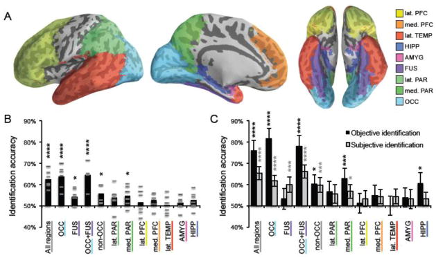
Identification accuracy for reconstructed faces by ROI. (A) Using a standard space brain atlas, nine anatomical ROIs were generated, corresponding to: lateral prefrontal cortex (lat. PFC), medial prefrontal cortex (med. PFC), lateral temporal cortex (lat. TEMP), hippocampus (HIPP), amygdala (AMYG), fusiform gyrus (FUS), lateral parietal cortex (lat. PAR), medial parietal cortex (med. PAR), and occipital cortex (OCC). (B) Mean objective (Euclidean distance-based) identification accuracy for reconstructions generated from each participant (grey, horizontal lines) and the average across participants for each ROI (black, vertical bars). For each ROI, accuracy across participants was compared to chance performance (50%) via a one-sample t-test. (C) Black bars represent objective (Euclidean distance-based) identification accuracy for mean reconstructions (i.e., reconstructions averaged across participants). Error bars reflect the standard deviation in accuracy when the reconstruction labels were randomly permuted 100,000 times. Accuracy was compared to chance by measuring the proportion of times a randomly permuted set achieved greater accuracy than the reconstruction set itself. Grey bars represent subjective (human-based) identification accuracy for mean reconstructions. Error bars reflect standard error of the accuracy for each image (i.e., proportion of times it was chosen over the lure by an Amazon Mechanical Turk participant). Accuracy was compared to chance using a one-sample t-test of the null hypothesis that the accuracy of each image was distributed with mean 0.5. **** p < .001, *** p < .005, * p < .05.

The test of identification accuracy was also repeated using the mean reconstructions (i.e., for each test face, the mean of the reconstructed images generated from each of the six participants). Sample mean reconstructions for several ROIs are shown in Fig. 2 (see Fig. S3 for all mean reconstructions from the all regions ROI). Objective (Euclidean distance-based) identification accuracy for the mean reconstructions was higher than for individual participants’ reconstructions: all regions, M = 76.2%; occipital, 81.7%; non-occipital, 60.3% (Fig. 3C). Thus, by combining reconstructions generated by distinct participants, a notable increase in reconstruction quality was observed. To test whether accuracies for the mean reconstructions were significantly above chance, permutation tests were conducted in which, prior to calculating Euclidean distance-based accuracy, the mapping between each test image and its corresponding neural reconstruction was randomly permuted (switched) such that a given test image was equally likely to be associated with each of the 30 reconstructions. This process was repeated until 100,000 different random permutations had been tested, generating a chance distribution of Euclidean distance-based accuracy. Thus, for individual brain masks, the probability of obtaining the observed Euclidean distance-based accuracy under the null hypothesis could be expressed as the proportion of times (n/100,000) that an accuracy at least that high was observed in the random permutations. For each of our core brain masks, observed accuracy was significantly above chance: all regions, p < .00001; occipital p < .00001; non-occipital p = .01.

Figure 2.

Reconstructions, averaged across participants, from various ROIs. Each row corresponds to a test face seen by each participant; the actual (original) image seen by the participant is shown in the left column. The ‘non-neural’ PCA reconstruction is shown in the second column from left. Note: “all regions” refers to the 9 ROIs shown in Figure 3A; “all non-occipital” refers to the “all regions” ROI minus the occipital ROI.

While the preceding analyses indicate that reconstructed test images could be identified (i.e., matched with the corresponding test image) based on pixel-by-pixel similarity in RGB values, this does not guarantee that the reconstructions were subjectively similar to the test images. Thus, we replicated the identification analyses described above with the exception that instead of a computer algorithm determining whether the target reconstruction was more similar to the test image than to a lure image, human participants now made this decision. Here, we only used the mean reconstructions (i.e. those generated by averaging across reconstructions from the 6 participants). Human responses were collected via Amazon’s Mechanical Turk. One response was collected for each of the 29 possible pairings, for each of the 30 test faces, and for each of 9 different brain masks. Each participant in the study made 30 ratings (one rating for each reconstructed test face). Thus, a total of 261 participants contributed 30 responses each, for a grand total of 7,830 responses collected (870 per brain mask). Again, accuracy of each individual reconstruction reflected the percentage of trials in which a human (participant) selected its corresponding test image over the lure. The average accuracy for a given brain mask was the average across all 29 pairings for the 30 reconstructions (870 total pairings).

Here, a human-based analog of the permutation test described above would not have been practical in that it would have required massive amounts of additional data collection. Instead, we computed the probability of obtaining the observed accuracy for each region via a single-tailed one-sample t-test in which accuracy for each of the 30 neural reconstructions (the proportion of 29 Mechanical Turk participants who chose the associated test face over the lure) was compared to chance performance of 50%, thus providing a test of whether reconstruction accuracy would generalize to new faces. Performance was significantly above chance in the all regions (p = .00001), occipital (p = .00002), and non-occipital (p = 0.004) ROIs, as well as in fusiform (p = 0.004), fusiform+occipital (p = .000005), and medial parietal (p = 0.02) (Fig. 3C). In addition, the reconstructions derived from the fusiform gyrus were associated with relatively greater subjective identification accuracy than objective identification accuracy, whereas the opposite was true for reconstructions from the occipital cortex (Fig. 3C). This interaction between region (fusiform vs. occipital) and verification method (subjective vs. objective) was highly significant (F_1,119 = 22.4, p < .0001; images treated as random effects).

Accuracy Heat Maps

The above results indicate that neural reconstructions of faces were objectively and subjectively similar to the original test faces. A secondary goal was to examine which parts of the faces reconstructed well. To address this, we re-ran the pixel-based identification analysis (where a target and lure reconstruction were compared to a test image based on Euclidean distance of pixel values), but this time measured Euclidean distance separately for the RGB components of each individual pixel. In other words, we computed the mean identification accuracy for each pixel. Pixel-by-pixel accuracy could then be plotted, yielding a ‘heat map’ that allowed for visualization of the regions that reconstructed well or poorly. This measurement was applied only to the mean reconstructions and was separately performed for five different brain masks. As can be seen in Fig. 4, pixels around the eyes (including eyebrows), mouth, and forehead all contributed to reconstruction accuracy. Notably, eye color and pupil location did not reconstruct well; however, this information is likely more subtle and less salient than facial expressions and affect, which would be more clearly captured by eyebrows and mouth shape. (In general, gaze direction might be one salient feature of the eyes, but because almost all of the test faces were gazing directly forward it is not a feature that was likely to contribute to reconstruction accuracy).

Figure 4.

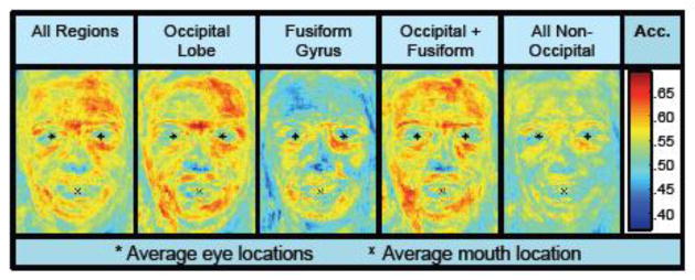
Mean objective (Euclidean distance-based) identification accuracy of each pixel in reconstructed face images from 5 different regions. High accuracy at an individual pixel location indicates that image information at that pixel positively contributed to identification accuracy.

Neural Importance Maps

Thus far we have considered the accuracies of reconstructions generated using a (near) whole-brain mask as well as various broad anatomical regions of interest. We next sought to identify the specific, ‘local’ clusters of voxels that were most important for generating face reconstructions. To this end, the PLSR training algorithm was repeated using the “all regions” ROI, but without any voxel selection. The backward model mapping neural activation to face components was then transformed into a forward model mapping face components to neural activation according to a method recently described by Haufe and colleagues (2014; see equation 6). However, to correct for the fact that weights were inversely proportional to the magnitude of component scores (meaning that late components with small magnitudes were assigned large weights), we multiplied the weight for each component by the variance of the corresponding component scores. As a result, the weights for each component were proportional to the magnitude of component scores (as was the case in the backward model). The model weights were then averaged for each component across all six subjects. Finally, to produce a single value reflecting the overall importance of each voxel, we calculated the root mean square weight for each voxel across the 299 components.

The resulting mean model weights constitute an “importance map,” with higher values corresponding to voxels that were more predictive of face components. Notably, the motivation for generating the importance map was not to test which voxels ‘significantly’ contributed to reconstruction accuracy, but instead to provide a visualization of the voxels that were most important for generating reconstructions. For display purposes, we selected an arbitrary threshold of .175 times the maximum weight (i.e., only displaying voxels for which the mean weight exceeded this value), which was equivalent to selecting the 3117, or 9.05%, most ‘important’ voxels. As can be seen in Fig. 5A–C, clusters of ‘important’ voxels were located not only in early visual areas, but also in several areas that have previously been associated with face processing. For example, clusters were observed in mid to posterior fusiform gyrus, medial prefrontal cortex, angular gyrus/posterior superior temporal sulcus, and precuneus.

Figure 5.

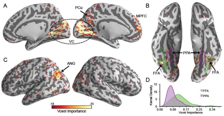
(A–C) “Importance map” of voxels on a standard space brain atlas. The model weight for each voxel and each component was averaged across the six subjects. Then, the root mean square regression weight for each voxel was taken across the 299 components. The resulting “importance” values are scaled such that their maximum is equal to 1. The map is thresholded at .175, displaying the top 3117 (or 9.05%) most important voxels. The most prominent clusters were observed in angular gyrus (ANG), fusiform gyrus (FG), medial prefrontal cortex (MPFC), precuneus (PCu), and visual cortex (VC). (B) Purple and green outlines delineate functional ROIs generated from a prior study (Kuhl et al., 2013) corresponding to face-selective regions of fusiform gyrus (FFA; green) and scene-selective regions near the collateral sulcus (PPA; purple). (D) Kernel smoothing estimates (bandwidth = .015) of the probability density of voxel “importance” values in FFA and PPA.

To more explicitly determine whether the clusters revealed by the importance map overlap with typical face processing regions, we used data from an independent, previously described study (Kuhl et al., 2013) to generate group-level functional ROIs representing (a) face-selective voxels in the fusiform gyrus (fusiform face area; FFA) and (b) scene-selective voxels centered on the collateral sulcus (parahippocampal place area; PPA). Specifically, we selected voxels in bilateral fusiform gyrus that were more active for face encoding than scene encoding (p < .001, uncorrected; 185 voxels total) and voxels at/near the collateral sulcus that were more active for scene encoding than face encoding [p < 10⁻¹⁰, uncorrected, which yielded an ROI roughly the same size as the fusiform face ROI (222 voxels)]. As can be seen in Fig. 5B, the importance map revealed clusters that fell within FFA but not in PPA. Moreover, comparing the kernel densities of voxel importance in these two regions confirmed that FFA voxels were generally more important than PPA voxels (Fig. 5D). Notably, overlap between the importance map and face-selective regions (generated from the previous data set) was also evident in several other regions: medial prefrontal cortex, precuneus, and angular gyrus (Fig. S4).

Removing Low-Level Visual Information

Because our test images (and training images) differed in terms of color, luminance, and contrast, one concern is that reconstruction accuracy was driven by low-level properties. Indeed, previous studies have shown that even high-level visual regions such as the fusiform face area can be sensitive to low-level visual properties (Yue et al., 2011). To address this concern, we re-ran the PLSR algorithm using components generated from a PCA analysis of face images for which color, luminance, and contrast differences were removed. First, each face image was converted to grayscale by averaging across the three color channels. Each image was also cropped more tightly (34 pixels from the top, 10 pixels from the bottom, and 9 pixels from each side were removed) to eliminate some remaining background information in the images that would have influenced luminance normalization. Next, the pixel values were mapped to 64 discrete gray levels such that, for each face, roughly the same number of pixels occupied each level of gray. In other words, after this transformation, the histograms of pixel intensity values for each image were equivalent (i.e., a uniform distribution for each image) and, therefore, the mean and variance of pixel intensity values across images were nearly identical. Thus, even though participants saw face images that differed in low-level information such as color, contrast, and luminance, the algorithm was ‘blind’ to this information and thus could not support reconstruction of this information.

Even with color, luminance and contrast information removed (Fig. 6A), reconstruction accuracy generally remained robust. “Objective” accuracies for the reconstructions based on normalized images were still above chance in the “all regions” ROI (M = 70.6%; p < .0001), occipital (M = 68.62%; p < .001) and non-occipital (M = 65.3%; p < .001) (Fig. 6B). “Subjective” accuracies (collected via Mechanical Turk: 30 ratings per subject * 29 unique image pairings * 3 ROIs = 2610 ratings) were above chance in the “all regions” ROI (M = 59.2%; p < .001) and occipital ROI (M = 60.1%, p < .0001). Thus, while some low-level information (e.g., skin tone) is likely related to high-level face processing, the present reconstruction results cannot be explained in terms of low-level differences in color, luminance, and contrast. In fact, the normalized-image reconstructions derived from the non-occipital ROI were associated with relatively greater objective identification accuracy than the reconstructions based on non-normalized images. The opposite was true for reconstructions from the occipital cortex: relatively greater objective identification accuracy for the reconstructions derived from non-normalized, relative to normalized, images. The interaction between region (OCC vs. non-OCC) and normalization was significant (F_1,119 = 11.1, p < .005; images treated as random effects). Thus, while color, luminance, and contrast information in the face images may have modestly improved reconstructions generated from occipital cortex, it did not contribute to reconstructions generated from non-occipital regions.

Figure 6.

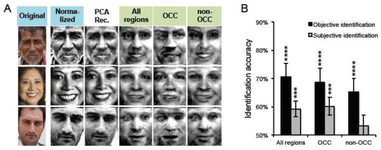
(A) Example test images in their original form (left column), normalized form (second column from left) form, and the ‘non-neural’ PCA reconstructions (third column from left), alongside reconstructions from three regions of interest: all regions, occipital (OCC), and non-occipital (non-OCC). (B) Mean “objective” and “subjective” identification accuracies for reconstructions based on normalized images from the three regions of interest. For an explanation of the error bars and of how accuracy was compared to chance, see Figure 3C. **** p < .001, *** p < .005.

Pattern Similarity Approach

Though the method of reconstructing perceived faces from their evoked brain activity by predicting their eigenface coefficients is clearly effective, it is possible that computationally simpler methods could achieve similar success. In particular, we were interested in whether perceived faces could be ‘reconstructed’ by simply selecting the training face (or averaging a set of training faces) that elicited similar patterns of brain activity.

To this end, reconstructions were produced by averaging the first N training face images whose corresponding brain activity was most similar to that associated with a given test face, where Pearson’s product-moment correlation coefficient was used to assess similarity. This was performed separately for each participant and brain mask. The reconstructions of a given test face from each subject were averaged together (i.e., across subjects) and their difference from the mean image was multiplied by the square root of 6xN and added back into the mean image (as with the PCA based reconstructions, but accounting for the fact that the mean image is now the average of 6xN images). The accuracy of the resulting set of reconstructions was assessed via the same Euclidean distance-based matching task that was used to assess the PCA-based neural reconstructions. The accuracies of similarity-based neural reconstructions are shown in Fig. 7, where N varies from 1 (selecting the single most similar face) to 300 (selecting all training faces). P-values were computed via the same permutation-based hypothesis test that was used to evaluate the PCA-based reconstructions.

Figure 7.

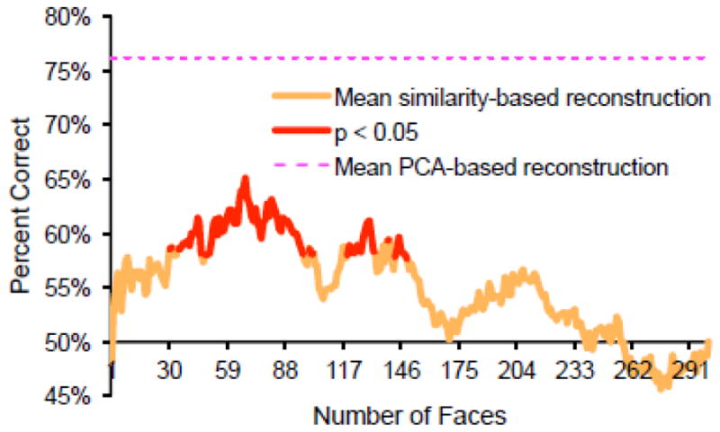
Mean objective identification accuracy of similarity-based reconstructions (averaged across participants). Accuracy is plotted as a function of the number of faces included (averaged across) in the reconstruction. For example, identification accuracy when n = 60 refers to accuracy based on a reconstruction that equals the average of the 60 training faces that elicited the most similar pattern of activity to a given test face. Statistical significance was again established by randomly permuting the labels on the reconstructed images 100,000 times and measuring the proportion of times a randomly permuted set achieved greater accuracy than the reconstruction set itself. Mean accuracy of the PCA-based mean reconstructions (from the all regions ROI) is shown for comparison (dashed, magenta line).

Although there was a moderately large number of values of N for which the similarity-based neural reconstructions were significantly above chance (without correcting for the fact that there were 300 comparisons) (Fig. 7), even the peak accuracy of these reconstructions (when N = 68 faces; Fig. S5) was far lower than the accuracy of the PCA-based reconstructions from the same voxels (shown, for comparison, in Fig. 7). In particular, it is evident that selecting the single most similar training face as a ‘reconstruction’ was not effective at all. While we believe these results clearly highlight the advantage of the PCA-based reconstruction approach, it should be noted that the relative difference between the PCA-based approach and a similarity-based approach would potentially vary as a function of the number of times each training face was presented as well as the total number of unique images—factors we cannot explore in the present study.

DISCUSSION

Here, we used a machine learning algorithm to map distributed patterns of neural activity to higher-order statistical patterns contained within face images. We then used these mappings to reconstruct, from evoked patterns of neural activity, face images viewed by human participants. Our results provide a striking confirmation that face images can be reconstructed from brain activity both within and outside of occipital cortex. The fidelity of the reconstructions was validated both by an objective comparison of the pixel information contained within the original and reconstructed face images and by having human observers subjectively identify the reconstructed faces. While the limited number of neural reconstruction studies to date have had the same essential motive—to provide a direct (and frequently remarkable) visual representation of what someone is seeing—the present study is novel in terms of the neural regions from which reconstructions were generated, the specific methods (including stimulus class) used for reconstruction, and the potential applications of the results. We consider each of these points below.

Reconstructions from higher-level brain regions

Prior neural reconstruction studies have relied almost exclusively upon retinotopically organized activity in early visual regions (V1, V2); exceptions include reconstructions of natural scenes that were based on both early and late visual areas of occipital cortex (Naselaris et al., 2009) and reconstructions of isolated color information based on intermediate visual areas (e.g., V4) (Brouwer and Heeger, 2009). Thus, an important aspect of our findings is that we achieved reliable reconstruction accuracy even when excluding all of occipital cortex. While there is at least some degree of retinotopic organization outside of occipital cortex (Hemond et al., 2007), reconstructions generated when excluding occipital cortex are less likely to be based on retinotopically organized information. Indeed, while the actual form of the reconstructions we produced was ‘visual’, it is likely that these reconstructions were partly driven by patterns of activity representing semantic information (Huth et al., 2012; Mitchell et al., 2008; Stansbury et al., 2013).

The reconstructions derived from the fusiform gyrus are particularly interesting in that they were associated with relatively greater subjective identification accuracy (i.e. via human recognition) than objective identification accuracy (via pixel-based Euclidean distance), whereas the opposite was true for reconstructions from the occipital cortex (Fig. 3C). This dissociation is consistent with evidence that the fusiform gyrus is more involved in subjective aspects of face processing than occipital regions (Fox, Moon et al., 2009). For example, activity in the fusiform face area (FFA)—but not the occipital face area (OFA)—is related to participants’ subjective perceptions of face identity and facial expression, whereas activity in the OFA tracks structural changes but does not distinguish between different subjective perceptions of identity and expression (Fox, Moon et al., 2009). Our success in deriving reconstructions from the fusiform gyrus also provides evidence that activity patterns in the fusiform gyrus differentiate between distinct face images. Whether the face representations in fusiform gyrus were also identity specific (Verosky et al., 2013)—that is, whether different images of the same identity would yield similar reconstructions—cannot be established here since each face image that we used corresponded to a distinct identity. However, future studies could test for identity-specific information by varying viewpoint (Anzellotti et al., 2013). For example, if training faces used for PCA were forward-facing and test faces varied in viewpoint, reconstructions would also be forward-facing, and could therefore only represent information that is retained across changes in viewpoint. [Transient facial features such as emotional expression (Nestor et al., 2011) could be varied in a similar fashion.]

Our importance map confirmed that in addition to early visual regions, clusters within fusiform gyrus also predicted face components. The localization of these clusters was consistent with what is typically labeled as FFA. Indeed, these clusters overlapped with independently identified group-level functional ROIs representing face-selective fusiform voxels. As a comparison, we confirmed that face-selective voxels in fusiform gyrus were more important in predicting face components than were scene-selective voxels in the collateral sulcus. A number of other functionally-defined face regions also overlapped with clusters within the importance map: (a) medial prefrontal cortex, (b) precuneus, and (c) angular gyrus/posterior superior temporal sulcus. These regions correspond to a broader network of areas that have been associated with various aspects of face processing (Fox, Iaria et al., 2009; Gobbini and Haxby, 2007). Thus, our results indicate that higher-level regions previously associated with face processing contributed to successful reconstruction of viewed faces. Notably, reconstruction from higher-level (non-occipital) regions was not driven by color, luminance, or contrast, as removal of this information from the images increased objective identification accuracy (whereas the opposite was true for reconstructions generated from occipital cortex).

Method of Reconstruction

Prior studies reporting neural reconstructions have used both encoding models (Naselaris et al., 2009) and decoding models (Miyawaki et al., 2008; Thirion et al., 2006). Encoding models attempt to predict the pattern of brain activity that a stimulus will elicit, whereas decoding methods involve predicting (from brain activity) features of the stimulus. Thus, our approach involved decoding; however, instead of predicting relatively simple information such as local contrast values (Miyawaki et al., 2008), here we predicted relatively complex information that was succinctly captured by PCA component scores (i.e., eigenface scores).

One appealing feature of our specific reconstruction approach, relative to that of previous studies, is that our selection of stimulus features (i.e., eigenfaces) was entirely unsupervised. That is, rather than using a manually selected local image basis such as a set of binary patches (Miyawaki et al., 2008) or Gabor filters (Naselaris et al., 2009; Nishimoto et al., 2011), and without applying any semantic labels to the images (Naselaris et al., 2009), we identified components that efficiently represented face images. While the derived components are likely to explain variance related to features such as gender, race, and emotional expression (Fig. S6 and S7), we did not need to subjectively define any of these categories. In fact, because we made virtually no assumptions about the type of face information that would be reflected in patterns of brain activity, the pixelwise maps of reconstruction accuracy shown in Fig. 4 represent a largely unconstrained account of what parts of the face were represented in brain activity, which would not have been the case if we had chosen to model particular features (e.g. eyes and mouth).

A second advantage of our PCA-based approach is that predicted component scores for an image can be easily inverted to produce a reconstruction, meaning that our method of neural reconstruction was very direct. That is, whereas the use of an image prior has been an important component of other studies reporting neural reconstruction of complex visual information (Naselaris et al., 2009; Nishimoto et al., 2011; Schoenmakers et al., 2013), here this was unnecessary. Third, having orthogonal components (eigenfaces) avoided complications that can arise with correlated features (i.e., that brain activity elicited by one feature is mistaken for brain activity elicited by another feature). Finally, our approach is computationally inexpensive because relatively few features or components were used in our PLS algorithm compared to the number of pixels in each image.

Given that we used the maximum number of eigenfaces (299) to generate reconstructions, it may be wondered whether later components actually contributed to reconstruction accuracy. For example, since the first two components captured 41.4% of the variance of the training faces and appeared to carry information about skin color, gender, and expression (where the latter two properties appeared to covary; Fig. S6 and S7), it might have been sufficient to use these first two components alone. However, even when the first two components were excluded from our model, identification accuracy for mean reconstructed images in the all regions ROI remained significantly above chance (M = 0.57; p = 0.005). Furthermore, as can be seen in Fig. 8A, qualitative differences in the reconstructed images are apparent even as relatively ‘late’ components are added. Indeed, while the first 10 components account for the majority of the objective identification accuracy of the reconstructions (Fig. 8B), there was a significant positive correlation between identification accuracy and the number of included components even when considering only components 11–299 (Fig. 8C). Thus, our results suggest that neural activity predicted both highly salient (early components) and more nuanced features (later components) of face images.

Figure 8.

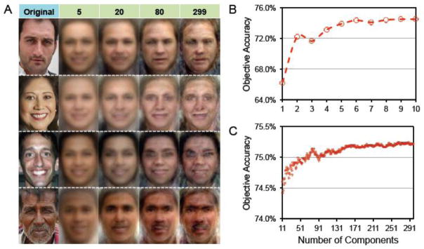
(A) Mean (across participant) reconstructions from the all regions ROI as a function of the number of components (eigenfaces) used for reconstruction. (B,C) Objective accuracy of mean reconstructions from all regions ROI as a function of the number of components (eigenfaces) used for reconstruction. Here, instead of comparing each reconstruction with 29 lures (the other test faces), each reconstruction was compared to 329 lures (every training and test face) to attain a more stable measure of accuracy (i.e., to decrease error variance of each measurement by a factor of 329/29). This was not done in previous analyses because, if the test faces were systematically different from the training faces, this could bias accuracy (relative to chance)—but the present analysis was not concerned with performance relative to chance. For components 1 through 10 (B), Spearman’s rank correlation between the number of components included and accuracy was 0.97. For components 11 through 299 (C), Spearman’s rank correlation between number of components included and accuracy was 0.95. These correlation values cannot be compared to chance in the traditional way because the accuracies are clearly non-independent (e.g., the accuracy when using 251 components will be extremely close to the accuracy when using 250 components). Thus, to compute a p-value for the correlation, r, for components 11 through 299, we performed a 5-step non-parametric test: (1) we evaluated the discrete derivative (differences between adjacent elements, which can be assumed to be statistically independent in this case) of accuracy as a function of number of components, (2) we multiplied this by a random string of −1 and 1 values, (3) we cumulatively summed this function and computed the correlation (r′) of the result (starting at 0) with the number of components, (4) steps 2–3 were repeated 100,000 times, and (5) finally, we calculated the proportion of instances in which r′ (the correlation generated in step 3) was greater than r (the actual correlation between number of components included and accuracy). The resulting p-value was 0.0091. Thus, with the addition of components 11–299, accuracy increased in a roughly monotonic fashion, though the magnitude of this increase was very small.

While our results highlight the utility of PCA as a tool for extracting face information in a fully automated, data-driven way (Turk and Pentland, 1991), here we are not advancing the stronger position that the brain represents faces using a linear projection onto features that strongly resemble PCA components. Rather, it is possible that the brain uses a wholly different (e.g., nonlinear) transformation to represent faces. However, our method of face reconstruction is based on the idea that at least some aspects of the brain’s representations of faces will correlate with, or predict, the PCA components of faces (Gao and Wilson, 2013). Future studies could compare different methods for representing faces in a low-dimensional space (e.g., principal components analysis vs. independent components analysis) or could systematically compare reconstruction of individual eigenfaces across different brain regions as a way to probe the underlying dimensions of the brain’s representation of faces.

Our method of reconstructing face images can also be compared to previous studies that have used decoding methods to study face processing. Previous face decoding studies have used just a handful of face identities (Anzellotti et al., 2013; Kriegeskorte et al., 2007; Nestor et al., 2011; Verosky et al., 2013) or faces that were artificially varied along a handful of dimensions (Gao and Wilson, 2013; Goesaert and Op de Beeck, 2013). By contrast, the present study employed naturalistic images featuring a large number of distinct identities and was not constrained to a limited number of selected features. Rather, our approach would allow for any number of face features to be reconstructed, but also automatically selects those features that explain the most variance across faces images.

Applications

Our approach has a number of direct applications. First, as we demonstrate here, reconstructions can be generated and compared across different brain regions, allowing for a strikingly direct method of assessing what face information is represented in each region. Likewise, reconstructions could also be compared across specific populations or groups, allowing for comparison of how face representations differ across individuals. This would be particularly relevant to disorders such as autism that have been associated with abnormal face processing. (The accuracy “heat maps” we report in Fig. 4 could be quite useful for such comparisons). Reconstructions of faces could also be used to assess implicit biases in perception, since a face can be reconstructed in the absence of a participant making any behavioral response to that image. For example, manipulations that are intended to induce racial prejudice or social anxiety might correspond to discernable differences in the reconstructed faces (e.g. darker skin color or more aggressive facial expression). This application is especially promising in light of the role of high-level face processing areas in implicit biases (Brosch et al., 2013).

Finally—and perhaps most intriguingly—our method could, in principle, be used to reconstruct faces in the absence of visual input. As noted above, prior studies reporting neural reconstructions have largely relied on mapping voxel activity to information at a particular retinotopic location. However, voxels in higher-level regions (e.g., fusiform gyrus) are likely to represent face information in a way that is invariant to position (Kovács et al., 2008) and at least partially invariant to viewpoint (Axelrod and Yovel, 2012). While our method requires that the training faces be carefully aligned—so that PCA can be applied to the images—it does not place any requirements on the format of the test images. For example, had the test images been twice the size of the training images, reconstructions based on ‘higher-level’ representations would still succeed—the reconstructed image would simply be projected into the same space as the training images. Similarly, the current approach could be applied, without any modification, to attempt reconstructions of faces that were imagined, dreamed, or retrieved from memory. Indeed, recent studies have found that the visual content of imagery (Stokes et al., 2011), memory retrieval (Kuhl et al., 2011; Polyn et al., 2005), and dreams (Horikawa et al., 2013) are represented in higher-level visual areas—areas that overlap with those that supported face reconstruction in the present study. Thus, extending the present methods to reconstruction of off-line visual information represents a truly exciting—yet theoretically feasible—avenue for future research.

Highlights.

• We used PCA to identify components that represent face images (eigenfaces)

• Eigenfaces were mapped to fMRI activity patterns using machine learning

• Activity patterns elicited by novel faces were used to reconstruct face images

• Neural reconstructions of faces were objectively and subjectively identifiable

References

- Anzellotti S, Fairhall SL, Caramazza A. Decoding representations of face identity that are tolerant to rotation. Cereb Cortex. 2013 doi: 10.1093/cercor/bht046. http://dx.doi.org/10.1093/cercor/bht046. [DOI] [PubMed]
- Axelrod V, Yovel G. Hierarchical processing of face viewpoint in human visual cortex. J Neurosci. 2012;32:2442–2452. doi: 10.1523/JNEUROSCI.4770-11.2012. [DOI] [PMC free article] [PubMed] [Google Scholar]
- Brosch T, Bar-David E, Phelps EA. Implicit race bias decreases the similarity of neural representations of black and white faces. Psychol Sci. 2013;24:160–166. doi: 10.1177/0956797612451465. [DOI] [PMC free article] [PubMed] [Google Scholar]
- Brouwer GJ, Heeger DJ. Decoding and reconstructing color from responses in human visual cortex. J Neurosci. 2009;29:13992–14003. doi: 10.1523/JNEUROSCI.3577-09.2009. [DOI] [PMC free article] [PubMed] [Google Scholar]
- Donato G, Bartlett MS, Hager JC, Ekman P, Sejnowski TJ. Classifying facial actions. IEEE Trans Pattern Anal Mach Intell. 1999;21:974–989. doi: 10.1109/34.799905. [DOI] [PMC free article] [PubMed] [Google Scholar]
- Fox CJ, Iaria G, Barton JJS. Defining the face processing network: optimization of the functional localizer in fMRI. Hum Brain Mapp. 2009;30:1637–1651. doi: 10.1002/hbm.20630. [DOI] [PMC free article] [PubMed] [Google Scholar]
- Fox CJ, Moon SY, Iaria G, Barton JJ. The correlates of subjective perception of identity and expression in the face network: An fmri adaptation study. NeuroImage. 2009;44:569–580. doi: 10.1016/j.neuroimage.2008.09.011. [DOI] [PMC free article] [PubMed] [Google Scholar]
- Gao X, Wilson HR. The neural representation of face space dimensions. Neuropsychologia. 2013;51:1787–1793. doi: 10.1016/j.neuropsychologia.2013.07.001. [DOI] [PubMed] [Google Scholar]
- Gauthier I, Tarr MJ, Moylan J, Skudlarski P, Gore JC, Anderson AW. The fusiform “face area” is part of a network that processes faces at the individual level. J Cogn Neurosci. 2000;12:495–504. doi: 10.1162/089892900562165. [DOI] [PubMed] [Google Scholar]
- Goesaert E, Op de Beeck HP. Representations of facial identity information in the ventral visual stream investigated with multivoxel pattern analyses. J Neurosci. 2013;33:8549–8558. doi: 10.1523/JNEUROSCI.1829-12.2013. [DOI] [PMC free article] [PubMed] [Google Scholar]
- Hart AJ, Whalen PJ, Shin LM, McInerney SC, Fischer H, Rauch SL. Differential response in the human amygdala to racial outgroup vs. ingroup face stimuli. NeuroReport. 2000;11:2351–2354. doi: 10.1097/00001756-200008030-00004. [DOI] [PubMed] [Google Scholar]
- Haufe S, Meinecke F, Görgen K, Dähne S, Haynes JD, Blankertz B, Bießmann F. On the interpretation of weight vectors of linear models in multivariate neuroimaging. NeuroImage. 2014;87:96–110. doi: 10.1016/j.neuroimage.2013.10.067. [DOI] [PubMed] [Google Scholar]
- Hemond CC, Kanwisher NG, Op de Beeck HP. A preference for contralateral stimuli in human object- and face-selective cortex. PLoS ONE. 2007;2:e574. doi: 10.1371/journal.pone.0000574. [DOI] [PMC free article] [PubMed] [Google Scholar]
- Horikawa T, Tamaki M, Miyawaki Y, Kamitani Y. Neural decoding of visual imagery during sleep. Science. 2013;340:639–642. doi: 10.1126/science.1234330. [DOI] [PubMed] [Google Scholar]
- Huang GB, Jain V, Learned-Miller E. Unsupervised joint alignment of complex images. International Conference on Computer Vision (ICCV) 2007 [Google Scholar]
- Huth AG, Nishimoto S, Vu AT, Gallant JL. A continuous semantic space describes the representation of thousands of object and action categories across the human brain. Neuron. 2012;76:1210–1224. doi: 10.1016/j.neuron.2012.10.014. [DOI] [PMC free article] [PubMed] [Google Scholar]
- Kanwisher N, McDermott J, Chun MM. The fusiform face area: A module in human extrastriate cortex specialized for face perception. J Neurosci. 1997;17:4302–4311. doi: 10.1523/JNEUROSCI.17-11-04302.1997. [DOI] [PMC free article] [PubMed] [Google Scholar]
- Kovács G, Cziraki C, Vidnyánszky Z, Schweinberger SR, Greenlee MW. Position-specific and position-invariant face aftereffects reflect the adaptation of different cortical areas. NeuroImage. 2008;43:156–164. doi: 10.1016/j.neuroimage.2008.06.042. [DOI] [PubMed] [Google Scholar]
- Kriegeskorte N, Formisano E, Sorger B, Goebel R. Individual faces elicit distinct response patterns in human anterior temporal cortex. Proc Natl Acad Sci USA. 2007;104:20600–20605. doi: 10.1073/pnas.0705654104. [DOI] [PMC free article] [PubMed] [Google Scholar]
- Krishnan A, Williams LJ, McIntosh AR, Abdi H. Partial least squares (PLS) methods for neuroimaging: A tutorial and review. NeuroImage. 2011;56:455–475. doi: 10.1016/j.neuroimage.2010.07.034. [DOI] [PubMed] [Google Scholar]
- Kuhl BA, Johnson MK, Chun MM. Dissociable neural mechanisms for goal-directed versus incidental memory reactivation. J Neurosci. 2013;33:16099–16109. doi: 10.1523/JNEUROSCI.0207-13.2013. [DOI] [PMC free article] [PubMed] [Google Scholar]
- Kuhl BA, Rissman J, Chun MM, Wagner AD. Fidelity of neural reactivation reveals competition between memories. Proc Natl Acad Sci USA. 2011;108:5903–5908. doi: 10.1073/pnas.1016939108. [DOI] [PMC free article] [PubMed] [Google Scholar]
- McIntosh AR, Bookstein FL, Haxby JV, Grady CL. Spatial pattern analysis of functional brain images using partial least squares. NeuroImage. 1996;3:143–157. doi: 10.1006/nimg.1996.0016. [DOI] [PubMed] [Google Scholar]
- Mitchell TM, Shinkareva SV, Carlson A, Chang KM, Malave VL, Mason RA, Just MA. Predicting human brain activity associated with the meanings of nouns. Science. 2008;320:1191–1195. doi: 10.1126/science.1152876. [DOI] [PubMed] [Google Scholar]
- Miyawaki Y, Uchida H, Yamashita O, Sato MA, Morito Y, Tanabe HC, Sadato N, Kamitani Y. Visual image reconstruction from human brain activity using a combination of multiscale local image decoders. Neuron. 2008;60:915–929. doi: 10.1016/j.neuron.2008.11.004. [DOI] [PubMed] [Google Scholar]
- Naselaris T, Prenger RJ, Kay KN, Oliver M, Gallant JL. Bayesian reconstruction of natural images from human brain activity. Neuron. 2009;63:902–915. doi: 10.1016/j.neuron.2009.09.006. [DOI] [PMC free article] [PubMed] [Google Scholar]
- Nestor A, Plaut DC, Behrmann M. Unraveling the distributed neural code of facial identity through spatiotemporal pattern analysis. Proc Natl Acad Sci USA. 2011;108:9998–10003. doi: 10.1073/pnas.1102433108. [DOI] [PMC free article] [PubMed] [Google Scholar]
- Nishimoto S, Vu AT, Naselaris T, Benjamini Y, Yu B, Gallant JL. Reconstructing visual experiences from brain activity evoked by natural movies. Curr Biol. 2011;21:1641–1646. doi: 10.1016/j.cub.2011.08.031. [DOI] [PMC free article] [PubMed] [Google Scholar]
- Polyn SM, Natu VS, Cohen JD, Norman KA. Category-specific cortical activity precedes retrieval during memory search. Science. 2005;310:1963–1966. doi: 10.1126/science.1117645. [DOI] [PubMed] [Google Scholar]
- Puce A, Allison T, Bentin S, Gore JC, McCarthy G. Temporal cortex activation in humans viewing eye and mouth movements. J Neurosci. 1998;18:2188–2199. doi: 10.1523/JNEUROSCI.18-06-02188.1998. [DOI] [PMC free article] [PubMed] [Google Scholar]
- Schoenmakers S, Barth M, Heskes T, van Gerven M. Linear reconstruction of perceived images from human brain activity. NeuroImage. 2013;83:951–961. doi: 10.1016/j.neuroimage.2013.07.043. [DOI] [PubMed] [Google Scholar]
- Smith ML, Gosselin F, Schyns PG. Measuring internal representations from behavioral and brain data. Curr Biol. 2012;22:191–196. doi: 10.1016/j.cub.2011.11.061. [DOI] [PubMed] [Google Scholar]
- Stansbury DE, Naselaris T, Gallant JL. Natural scene statistics account for the representation of scene categories in human visual cortex. Neuron. 2013;79:1025–1034. doi: 10.1016/j.neuron.2013.06.034. [DOI] [PMC free article] [PubMed] [Google Scholar]
- Stokes M, Saraiva A, Rohenkohl G, Nobre AC. Imagery for shapes activates position-invariant representations in human visual cortex. NeuroImage. 2011;56:1540–1545. doi: 10.1016/j.neuroimage.2011.02.071. [DOI] [PubMed] [Google Scholar]
- Thirion B, Duchesnay E, Hubbard E, Dubois J, Poline JB, Lebihan D, Dehaene S. Inverse retinotopy: Inferring the visual content of images from brain activation patterns. NeuroImage. 2006;33:1104–1116. doi: 10.1016/j.neuroimage.2006.06.062. [DOI] [PubMed] [Google Scholar]
- Turk MA, Pentland AP. Eigenfaces for recognition. J Cogn Neurosci. 1991;3:586–591. doi: 10.1162/jocn.1991.3.1.71. [DOI] [PubMed] [Google Scholar]
- Verosky SC, Todorov A, Turk-Browne NB. Representations of individuals in ventral temporal cortex defined by faces and biographies. Neuropsychologia. 2013;51:2100–2108. doi: 10.1016/j.neuropsychologia.2013.07.006. [DOI] [PMC free article] [PubMed] [Google Scholar]
- Whalen PJ, Rauch SL, Etcoff NL, McInerney SC, Lee MB, Jenike MA. Masked presentations of emotional facial expressions modulate amygdala activity without explicit knowledge. J Neurosci. 1998;18:411–418. doi: 10.1523/JNEUROSCI.18-01-00411.1998. [DOI] [PMC free article] [PubMed] [Google Scholar]
- Yue X, Cassidy BS, Devaney KJ, Holt DJ, Tootell RB. Lower-level stimulus features strongly influence responses in the fusiform face area. Cereb Cortex. 2011;21:35–47. doi: 10.1093/cercor/bhq050. [DOI] [PMC free article] [PubMed] [Google Scholar]
Associated Data
This section collects any data citations, data availability statements, or supplementary materials included in this article.