

Abstract
Purpose
Quantify the accuracy of a clinical proton treatment planning system (TPS) as well as Monte Carlo (MC) based dose calculation through measurements. Assess the clinical impact in a cohort of patients with tumors located in the lung.
Methods
A lung phantom and ion chamber array were used to measure the dose to a plane through a tumor embedded in lung and to determine the distal fall-off of the proton beam. Results were compared with TPS and MC calculations. Dose distributions in 19 patients (54 fields total) were simulated using MC and compared to the TPS algorithm.
Results
MC increases dose calculation accuracy in lung tissue compared to the TPS and reproduces dose measurements in the target to within ±2%. The average difference between measured and predicted dose in a plane through the center of the target is 5.6% for the TPS and 1.6% for MC. MC recalculations in patients show a mean dose to the clinical target volume on average 3.4% lower than the TPS, exceeding 5% for small fields. For large tumors MC also predicts consistently higher V5 and V10 to the normal lung, due to a wider lateral penumbra, which was also observed experimentally. Critical structures located distal to the target can show large deviations, though this effect is very patient-specific. Range measurements show that MC can reduce range uncertainty by a factor ~2: the average(maximum) difference to the measured range is 3.9mm(7.5mm) for MC and 7mm(17mm) for the TPS in lung tissue.
Conclusion
Integration of Monte Carlo dose calculation techniques into the clinic would improve treatment quality in proton therapy for lung cancer by avoiding systematic overestimation of target dose and underestimation of dose to normal lung. Additionally, the ability to confidently reduce range margins would benefit all patients through potentially lower toxicity.
Introduction
Proton Therapy is a rapidly growing treatment modality and continues to be investigated for new treatment sites, due its ability to provide superior dose distributions in many cases. Non-Small Cell Lung Cancer (NSCLC) has a high incidence rate with relatively poor patient outcomes and limited scope for dose escalation using conventional techniques (1).
Proton therapy has only relatively recently been investigated as a treatment modality for lung cancer (2). Various studies have reported promising results in terms of lower toxicity (3). A randomized phase II trial is underway (NCT00915005, clinicaltrials.gov) and more studies are currently recruiting (e.g. NCT01770418). The results of these ongoing studies and upcoming clinical trials will determine the future role of proton therapy in the treatment of lung cancer (4).
For photon dose calculations, it has long been known that equivalent-path-length (EPL) algorithms severely overestimate the dose to the target (5, 6). This has been the motivation for the development of alternative methods, such as convolution/superposition and Monte Carlo (MC) algorithms and their introduction into the clinic over the last decade (5). The adequacy of current clinical dose calculation algorithms for protons in this challenging geometry needs to be ensured. This deserves special attention, since the finite range of protons and the lower number of incident beam angles in proton compared to photon therapy leave less margin for error.
Our aims were to:
-
Assess a clinical TPS and a MC dose calculation algorithm through measurements in a lung phantom, focusing on:
-
1A
the dose to the target
-
1B
range uncertainties at the distal fall-off
-
1A
Analyze the difference between the TPS and MC in a cohort of 19 patients treated with passively scattered proton therapy
Materials & Methods
Patient Cohort
All patients undergoing proton therapy to treat tumors in the lung at our institution dating from July 2011 to July 2013 (n=18) were included in the study. Additionally, one patient that was planned with protons but randomized to the photon arm of an ongoing clinical trial was also included.
As this study focused on the accuracy of clinical dose calculations in the lung, the specific tumor histology did not impact the study design. Prescribed doses and fractionation schemes varied, the patient cohort included 6 stereotactic cases, 2 boost-plans complementing photon plans, and 11 fractionated schedules. To account for these variations, all deviations are given in percentages of the prescribed dose. Tumor sizes ranged from 2–318cc, with clinical stages from IA-IV.
To compare to a site with less complex patient geometry, an additional set of 10 liver fields from 5 cases, with similar water-equivalent ranges (108–194mm) and field sizes to the lung cohort was included.
Treatment Planning and Dose Calculation Algorithms
All patients were planned and treated using passively scattered proton therapy. The treatment planning system employed was XiO (Computerized Medical System) with an analytical algorithm based on (7). The patients were planned according to clinical protocols, either developed at our institution (8) or methods used in multi-institutional trials (9). For recalculation, the plans were exported from the TPS to the MC system TOPAS (TOol for PArticle Simulation) (10). Both TPS and MC dose calculations were based on identical Hounsfield Unit to relative stopping power relationships.
Phantom Study
Experiments were conducted at XXX. The Wellhofer I’mRT phantom consisted of 10mm slabs of cedar wood with a relative stopping power (SP) to water of 0.33, according to the HU-SP conversion curve used by the TPS. The tumor (20×20×20mm3, SP=1.15) is divided in two halves and embedded in two thicker slabs (20mm), to enable measurements in a plane within the target. Figure 1A shows the experimental setup. The structure placed on top of the 2D-array of ionization chambers (I’mRT MatriXX, Ion Beam Applications) is the middle part of the phantom, a CT scan of which is shown in Figure 1B. For all experiments we used the beam’s-eye-view x-ray system, reducing the setup uncertainty to <1mm. The uncertainty in dose measurement was assumed to be 1.5% according to vendor specifications, and the statistical uncertainty of the MC simulations was <1%, due to the high number of protons (108) simulated per field.
Fig. 1.

Experimental setup and results (A) Lung slabs (cedar wood) and chest wall (Lucite) positioned on the 2D-array of ionization chambers. (B) CT of the phantom with GTV (full) and CTV (dashed) contours. (C) Modified phantom with chest wall simulating a human ribcage, showing also the 2 halves of the embedded tumor in red. (D) Line profile through the central axis of the tumor, with magnifications for target periphery (E) and penumbra (F). Error bars for measurement 1.5%, for MC 1% (shaded blue).
We used the TPS to plan a treatment with a prescribed dose of 1Gy(RBE) to the clinical target volume (CTV), defined as 8mm expansion of the gross tumor volume (GTV). Subsequently, we delivered the treatment to the experimental setup (Figure 1A) and measured the dose distribution across a plane in the middle of the target.
For the range measurements, we modified the homogeneous phantom by including an artificial chest wall (Figure 1C), consisting of Lucite (20mm thickness) embedded with bone equivalent “ribs”. These ribs are have a diameter of 11mm and vary in spacing from 5–20mm to simulate the human ribcage with its increasing distance between the more inferiorly located ribs. Following clinical protocols, we developed a single-field treatment plan (range/modulation 9.1/4.4cm) to cover the target. 64 ionization chambers of the detector-array were located within the field. By gradually adding lung slabs (water-equivalent thickness=3mm) to the setup, we were able to measure the dose at each of these 64 points with increasing depth, allowing us to calculate the range in the phantom. We chose Range50, i.e. the range where the dose has fallen to 50% of the prescribed dose, to compare the measured and predicted ranges.
Results
Dose to target and normal lung
Figures 1D–F show the experimental results, obtained with the setup in Figures 1A–B, together with the predictions of the TPS and MC along a profile through the center of the target. The measurements in the periphery of the high dose region (Figure 1E) are consistently lower than planned by the TPS, within measurement uncertainty of the MC prediction. In the low-dose penumbra (Figure 1F) measurements and MC coincide as well, showing a higher dose than predicted by the TPS. Across the measurement plane within the target, the average difference between measurement and MC is 1.6% of prescribed dose, compared to 5.6% for the TPS.
The reason for the lower dose in the periphery, and conversely higher dose in the penumbra, is that protons interacting in the chest wall are scattered further out of field due to the low-density lung tissue that follows. The mechanism will be further discussed below.
A similar effect is observed in MC recalculations of patient treatment plans, shown in Figure 2A. The mean dose difference predicted by MC and TPS is plotted as a function of size of the aperture opening. The crosses represent the 54 fields from the 19 treatment plans and the circles correspond to the 10 liver fields. The MC algorithm consistently predicts a lower target dose, and the effect is higher in the lung compared to liver. The average(maximum) mean dose loss in is −2.3%(−5.4%) for all 54 fields. The measurement results from the experiment in Figure 1D are also indicated in Figure 2A, corresponding well to the Monte Carlo prediction. The minimum target dose for a specific field decreases by up to −7.6%. The average(maximum) mean dose loss per patient is −2.2%(−4.1%), as the effect averages out over multiple fields.
Fig. 2.
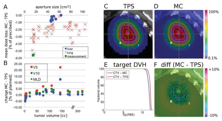
Summary of the patient study. (A) Mean target dose difference (MC-TPS) plotted against the size of the aperture opening. The measurement (green square) represents the average of (measurement-TPS) across the center of the CTV. (B) Changes in MLD, V5 and V10 in percent of planned values as a function of tumor volume, x-axis is broken for better visualization. (C–F) Example field: TPS dose (C), MC dose (D), DVHs (E) and dose difference (F=C–D). All color bars are percentages of prescribed dose, transparent <0.1%. Orange/blue contours represent the GTV/CTV.
Figure 2B demonstrates the effect of the calculation algorithm on the dose to normal lung, showing that MC predicts a lower dose to normal lung for small targets and a higher dose for large ones. The difference (MC-TPS) in mean lung dose (MLD) and the volumes receiving greater than 5Gy(RBE) (V5) and 10Gy(RBE) (V10) were between −5–+12%, −1–+22% and −4–+13% respectively.
Figures 2C–F show the results for one field of a lung patient, i.e. a single data point in Figure 2A. The TPS and MC predictions and their DVHs are shown in Figures 2C, 2D and 2E respectively. The dose difference in Figure 2F highlights the lower target dose predicted by MC. Note the increasingly lower dose towards the CTV edges in Figure 2F, which resembles the experimental results shown in Figure 1E.
Proton range
Figures 3A and 3B show the predictions of the TPS and the MC algorithms in the modified lung phantom which included an artificial chest wall. The difference between the two (MC-TPS) is shown in Figure 3C, with red and blue areas indicating higher doses in MC and TPS, respectively. The histograms in Figure 3D demonstrate the results, displaying the differences in Range50. Each entry represents the difference between predicted and measured range in one of the 64 measurement points on the distal surface. The average(maximum) range differences were 3.9mm(7.5mm) and 7mm(17mm) for MC and TPS respectively. Note that the range differences in Figure 3D are given in lung tissue, i.e. are magnified by a factor ~3 compared to soft tissue.
Fig. 3.
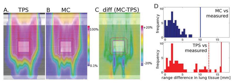
Experimental verification of proton range using a heterogeneous lung phantom (shown in Fig 1C): prediction of TPS (A), MC (B), difference MC-TPS (C). All color bars are percentages of prescribed dose, transparent <0.1%. (D) Histograms representing the difference in measured Range50 compared to MC (top, blue) and the TPS (bottom, red). The vertical lines represent range margins discussed in (20): 2.4%+1.2mm (solid blue), 4.6%+1.2mm (solid red), 3.5%+1mm (dashed red).
These differences are caused by inaccuracies in the modeling of multiple Coulomb scattering in the TPS algorithm, which only accounts for the material along each pencil’s central axis (11, 12). This effect is prominent when heterogeneities are along the beam path, which is the case for most lung patients due to rib-lung interfaces. Figure 4 shows the dose distribution calculated by the TPS, MC, their difference (MC-TPS) and the DVHs of target and the spinal cord (from left to right). This patient was ultimately treated with photons, however the data shows the impact range uncertainties can have. The increased range in the superior part of the field leads to a marked increase in dose to the spinal cord, which clearly alters the DVH.
Fig 4.
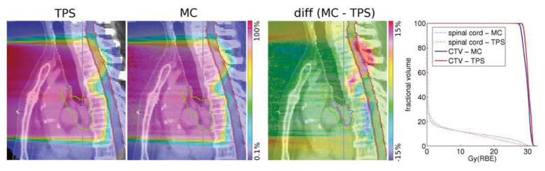
Example of underestimated range in a patient by an analytical dose calculation algorithm. All color bars are in percent of prescribed dose. Contours shown are the GTV (pink), CTV (green) and spinal cord (red).
Discussion
The experiments confirm that the dose delivered to peripheral regions of a target embedded in low-density tissue is lower than expected by the TPS and can be correctly predicted by MC simulations. The reason lies in the degradation of the lateral penumbra, which increases as a function of depth to a greater extent than is predicted by the TPS. XiO, as well as other treatment planning systems based on analytical algorithms (7, 11–13) assume that the penumbral width is a function of water-equivalent depth only. However, after scattering in the chest wall, the beam diverges over a longer distance, because of the higher geometric range of the beam in low-density tissue. The implication for the target dose is visualized in Figure 5A, which shows the dose profile as predicted by TPS and MC for the patient shown in Figures 2C–D, replicating the phantom results presented in Figures 1D–F.
Fig 5.
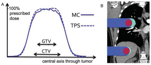
Left: Dose profile of TPS and MC along the horizontal axis of the dose distribution in Figures 2C–D Right: Visualization of the impact of tissue density on the range margin (cyan area). Both fields have the same (water-equivalent) range and therefore range margin, indicated in cyan, yet the margin of the superior field is enlarged by a factor ~3.
This effect is related to the well-known field-size-effect (14), which is exacerbated in low-density lung tissue. This is demonstrated by the liver fields also shown in Fig. 2A, which exhibit a similar size and range compared to the lung fields, yet do not show degradation in mean dose greater than 1%. This discrepancy of MC and analytical algorithms in lung compared to liver targets has already been noted in a recent study (15).
Impact of MC dose calculation on dose to target and critical structures
The dose reduction measured in the phantom, see Figure 1D, is similar to the in-patient effect predicted by MC (Figures 2C–F). The MC dose is slightly reduced compared to the TPS in the center, while towards the edge of the target the reduction becomes substantial (>5%), exceeding the dose tolerance typically required in the clinic.
As visible in Figure 2A, there is a significant correlation between the loss of mean target dose and the aperture size (Spearman’s p=0.0002). The spread among the values in Figure 2A for the same aperture size suggests additional confounding factors to the field-size (14). In addition to the aperture size, the distance between tumor and chest wall also significantly correlates (Spearman’s p=0.004) with lower dose. The range of the field also has a significant correlation (Spearman’s p=0.0001) to lower dose, though only for fields of similar size (>20cm2). Therefore fields with a large tumor-chest wall distance and a high range are most at risk of delivering lower target doses than predicted by the TPS.
As shown in the results, analytical dose calculation methods in the lung can lead to a mean dose loss in excess of 5% for small targets, while the lung V5 can increase by >20%. Not accounting for these deviations could inherently introduce bias into randomized clinical trials comparing photon and proton therapies for lung cancer.
First, due to the steep dose-response curve of most lung cancer cell lines (16), a lower mean target dose can have a significant effect on outcome, as shown in previous clinical studies(17). As Figure 5 demonstrates, the TPS underestimates the dose specifically in the CTV periphery, a region that has been linked to increased cancer stem cell density(18). Consequently, the effect on local control could be higher than the mean dose loss initially suggests. It has also been shown in clinical studies that prescription of dose to isocenter, leading to lower peripheral tumor doses, is linked to decreased local control(17).
Secondly, as the MC algorithm predicts consistently higher doses to the normal lung for large targets, conclusions regarding the toxicity of protons could be adversely affected. This would especially concern trials designed around iso-toxic dose escalation strategies(19).
Impact of MC dose calculation on range uncertainty and associated margins
The second area in which MC algorithms can impact clinical practice is through reduced range uncertainty margins. The impact will be greatest for large targets located in the lung, because the range margin is defined as an increase in the water-equivalent range. If the distal fall-off occurs in low-density tissue, as is shown in the right of Figure 5, the volume of normal tissue irradiated is increased compared to other soft-tissue sites.
It has been proposed that by employing MC algorithms for treatment planning, range margins associated with dose calculation uncertainty could be reduced from 4.6%+1.2mm to 2.4%+1.2mm (20), represented by the solid lines in Figure 3D. The results of this work indicate that the latter is an adequate margin for dose calculation uncertainty, though additional margins certainly have to be added to account for other uncertainties encountered in patient treatments. The lower histogram in Figure 3D suggests that 4.6%+1.2mm is a necessary margin for the current TPS. Furthermore, applying a margin of 3.5%+1mm, a commonly used value for proton range uncertainty (20), is not sufficient in this inhomogeneous geometry. Acknowledging this, we currently use additional range margins at our institution for lung treatments.
The reduction in range uncertainty margins by 2.2%, i.e. from 4.6% to 2.4%, can make a sizable difference if in lung tissue. For example, at 20cm range, MC algorithms could decrease the distal range margin by 4.4mm water-equivalent range, which corresponds to approximately 15mm of lung tissue.
Consequences & Future Directions
A possible short-term solution could be to triage patients to specific risk groups, as shown in figure 6. The left figure shows the fields divided into high risk (aperture<20cm2), intermediate risk (aperture>20cm2 and distance to chest wall>50mm) and low risk (aperture>20cm2 and distance to chest wall<50mm) groups. On the right side the delivered monitor units of the treatment fields are increased by 4% for high, 3% for intermediate and 2% for low risk, leading to a mean dose within 2% of prescription for all 54 fields. Another approach would be to perform retrospective MC dose calculation, particularly for patients with small tumors (aperture size<20cm2) located >50mm from the chest wall. The treatment plan could then be amended as required to counter the lower dose. Various scenarios can be envisioned as medium- to long-term solutions. Current shortcomings of analytical algorithms could be addressed in more advanced versions, such as pencil-beam redefinition algorithms (21), to improve the dose calculation accuracy in the presence of lateral heterogeneities.
Fig 6.
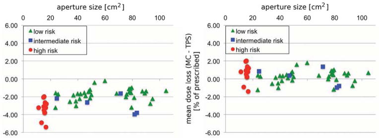
Possible mitigation approach applied to 54 treatment fields. Left: treatment fields divided into 3 risk groups, as described in the text. Right: treatment fields simulated with increased monitor units (high risk +4%, intermediate risk +3%, low risk +2%).
As the effects described in this publication are not the only weakness of current analytical algorithms (22, 23), the authors advocate the incorporation of MC algorithms into treatment planning. Monte Carlo algorithms have been the gold-standard for proton therapy dose calculation for decades (24), and the latest developments have shown promising results in terms of speed (25).
Though we studied the problem only for passively scattered proton therapy, the observed effect is a consequence of the shortcomings of current analytical algorithms, variants of which are employed by most clinical TPS. Therefore similar effects will likely be observed for active scanning proton therapy, which relies on these algorithms as well.
Conclusion
It has been demonstrated experimentally that current analytical dose calculation algorithms for protons used in the clinic can overestimate the mean dose to tumors situated in lung by over 5%, and underestimate the dose to the normal lung, especially V5 and V10. We strongly suggest Monte Carlo dose calculation as an integral part of any clinical proton therapy program focused on lung cancer, as there is strong evidence for the potential to reduce margins and increase the accuracy of the relationships between dose and effect, concerning tumor control as well as normal tissue toxicity. This is of ever-increasing importance, as the role of proton therapy in the treatment of lung cancer continues to be evaluated in clinical trials.
Summary.
We report on the assessment of the dose calculation accuracy for lung treatments with proton beams. A clinically used treatment planning system and Monte Carlo algorithm were compared with experiments in a heterogeneous lung phantom. The clinical impact of the differences was analyzed in a cohort of 19 patients. The results demonstrate that the clinical dose calculation algorithm overestimates the dose to the target, particularly if the tumor is small and centrally located.
Acknowledgments
This work was supported by National Cancer Institute Grant R01CA111590. The authors would like to acknowledge Dr. Henning Willers for fruitful discussions concerning clinical relevance, Dr. Ben Clasie for sharing his experimental expertise, Judy Adams and Nick Depauw for sharing their knowledge about treatment planning, and Dr. Jon Jackson and Partners Research Computing for maintenance of the computing cluster.
Footnotes
Conflict of Interest: none
Publisher's Disclaimer: This is a PDF file of an unedited manuscript that has been accepted for publication. As a service to our customers we are providing this early version of the manuscript. The manuscript will undergo copyediting, typesetting, and review of the resulting proof before it is published in its final citable form. Please note that during the production process errors may be discovered which could affect the content, and all legal disclaimers that apply to the journal pertain.
References
- 1.Chang JY, Zhang X, Wang X, et al. Significant reduction of normal tissue dose by proton radiotherapy compared with three-dimensional conformal or intensity-modulated radiation therapy in Stage I or Stage III non-small-cell lung cancer. Int J Radiat Oncol Biol Phys. 2006;65:1087–1096. doi: 10.1016/j.ijrobp.2006.01.052. [DOI] [PubMed] [Google Scholar]
- 2.Widesott L, Amichetti M, Schwarz M. Proton therapy in lung cancer: clinical outcomes and technical issues. A systematic review. Radiother Oncol. 2008;86:154–164. doi: 10.1016/j.radonc.2008.01.003. [DOI] [PubMed] [Google Scholar]
- 3.Chang JY, Komaki R, Wen HY, et al. Toxicity and patterns of failure of adaptive/ablative proton therapy for early-stage, medically inoperable non-small cell lung cancer. Int J Radiat Oncol Biol Phys. 2011;80:1350–1357. doi: 10.1016/j.ijrobp.2010.04.049. [DOI] [PMC free article] [PubMed] [Google Scholar]
- 4.Zips D, Baumann M. Place of Proton Radiotherapy in Future Radiotherapy Practice. Semin Radiat Oncol. 2013;23:149–153. doi: 10.1016/j.semradonc.2012.11.007. [DOI] [PubMed] [Google Scholar]
- 5.Chetty IJ, Curran B, Cygler JE, et al. Report of the AAPM Task Group No. 105: Issues associated with clinical implementation of Monte Carlo-based photon and electron external beam treatment planning. Med Phys. 2007;34:4818. doi: 10.1118/1.2795842. [DOI] [PubMed] [Google Scholar]
- 6.Knöös T, Ahnesjö A, Nilsson P, et al. Limitations of a pencil beam approach to photon dose calculations in lung tissue. Phys Med Biol. 1995;40:1411–1420. doi: 10.1088/0031-9155/40/9/002. [DOI] [PubMed] [Google Scholar]
- 7.XXX
- 8.XXX
- 9.Kang Y, Zhang X, Chang JY, et al. 4D Proton treatment planning strategy for mobile lung tumors. Int J Radiat Oncol Biol Phys. 2007;67:906–914. doi: 10.1016/j.ijrobp.2006.10.045. [DOI] [PubMed] [Google Scholar]
- 10.Perl J, Shin J, Schümann J, et al. TOPAS: An innovative proton Monte Carlo platform for research and clinical applications. Med Phys. 2012;39:6818. doi: 10.1118/1.4758060. [DOI] [PMC free article] [PubMed] [Google Scholar]
- 11.Petti PL. Differential-pencil-beam dose calculations for charged particles. Med Phys. 1992;19:137. doi: 10.1118/1.596887. [DOI] [PubMed] [Google Scholar]
- 12.Szymanowski H, Oelfke U. Two-dimensional pencil beam scaling: an improved proton dose algorithm for heterogeneous media. Phys Med Biol. 2002;47:3313–3330. doi: 10.1088/0031-9155/47/18/304. [DOI] [PubMed] [Google Scholar]
- 13.Ulmer W, Schaffner B. Foundation of an analytical proton beamlet model for inclusion in a general proton dose calculation system. Radiation physics and chemistry. 2011;80:378–389. [Google Scholar]
- 14.Daartz J, Engelsman M, Paganetti H, et al. Field size dependence of the output factor in passively scattered proton therapy: influence of range, modulation, air gap, and machine settings. Med Phys. 2009;36:3205–3210. doi: 10.1118/1.3152111. [DOI] [PubMed] [Google Scholar]
- 15.Yamashita T, Akagi T, Aso T, et al. Effect of inhomogeneity in a patient’s body on the accuracy of the pencil beam algorithm in comparison to Monte Carlo. Phys Med Biol. 2012;57:7673–7688. doi: 10.1088/0031-9155/57/22/7673. [DOI] [PubMed] [Google Scholar]
- 16.Das AK, Bell MH, Nirodi CS, et al. Radiogenomics predicting tumor responses to radiotherapy in lung cancer. Semin Radiat Oncol. 2010;20:149–155. doi: 10.1016/j.semradonc.2010.01.002. [DOI] [PMC free article] [PubMed] [Google Scholar]
- 17.Senthi S, Haasbeek CJA, Slotman BJ, et al. Outcomes of stereotactic ablative radiotherapy for central lung tumours: A systematic review. Radiother Oncol. 2013;106:276–282. doi: 10.1016/j.radonc.2013.01.004. [DOI] [PubMed] [Google Scholar]
- 18.Sottoriva A, Verhoeff JJC, Borovski T, et al. Cancer Stem Cell Tumor Model Reveals Invasive Morphology and Increased Phenotypical Heterogeneity. Cancer Res. 2010;70:46–56. doi: 10.1158/0008-5472.CAN-09-3663. [DOI] [PubMed] [Google Scholar]
- 19.van Elmpt W, De Ruysscher D, van der Salm A, et al. The PET-boost randomised phase II dose-escalation trial in non-small cell lung cancer. Radiother Oncol. 2012;104:67–71. doi: 10.1016/j.radonc.2012.03.005. [DOI] [PubMed] [Google Scholar]
- 20.Paganetti H. Range uncertainties in proton therapy and the role of Monte Carlo simulations. Phys Med Biol. 2012;57:R99–R117. doi: 10.1088/0031-9155/57/11/R99. [DOI] [PMC free article] [PubMed] [Google Scholar]
- 21.Egashira Y, Nishio T, Hotta K, et al. Application of the pencil-beam redefinition algorithm in heterogeneous media for proton beam therapy. Phys Med Biol. 2013;58:1169–1184. doi: 10.1088/0031-9155/58/4/1169. [DOI] [PubMed] [Google Scholar]
- 22.Sawakuchi GO, Titt U, Mirkovic D, et al. Monte Carlo investigation of the low-dose envelope from scanned proton pencil beams. Phys Med Biol. 2010;55:711–721. doi: 10.1088/0031-9155/55/3/011. [DOI] [PubMed] [Google Scholar]
- 23.Li Y, Zhu RX, Sahoo N, et al. Beyond Gaussians: a study of single-spot modeling for scanning proton dose calculation. Phys Med Biol. 2012;57:983–997. doi: 10.1088/0031-9155/57/4/983. [DOI] [PMC free article] [PubMed] [Google Scholar]
- 24.Carlsson AK, Andreo P, Brahme A. Monte Carlo and analytical calculation of proton pencil beams for computerized treatment plan optimization. Phys Med Biol. 1997;42:1033–1053. doi: 10.1088/0031-9155/42/6/004. [DOI] [PubMed] [Google Scholar]
- 25.Jia X, Schümann J, Paganetti H, et al. GPU-based fast Monte Carlo dose calculation for proton therapy. Phys Med Biol. 2012;57:7783–7797. doi: 10.1088/0031-9155/57/23/7783. [DOI] [PMC free article] [PubMed] [Google Scholar]