Three Dimensional Hadamard-encoded Proton Spectroscopic Imaging in the Human Brain using time-cascaded pulses at 3T

Abstract

PURPOSE

To reduce the specific-absorption-rate (SAR) and chemical shift displacement (CSD) of three dimensional (3D) Hadamard spectroscopic imaging (HSI) and maintain its point spread function (PSF) benefits.

METHODS

A 3D hybrid of 2D longitudinal, 1D transverse HSI (L-HSI, T-HSI) sequence is introduced and demonstrated in a phantom and the human brain at 3T. Instead of superimposing each of the selective Hadamard radio-frequency (RF) pulses with its N single-slice components, they are cascaded in time, allowing N-fold stronger gradients, reducing the CSD. A spatially refocusing 180° RF pulse following the T-HSI encoding block provides variable, arbitrary TE to eliminate undesirable short T₂ species’ signals, e.g., lipids.

RESULTS

The sequence yields 10–15% better signal-to-noise-ratio (SNR) and 8–16% less signal bleed than 3D chemical shift imaging of equal repetition time, spatial resolution and grid size. The 13±6, 22±7, 24±8 and 31±14 in vivo SNRs for myo-inositol, choline, creatine and N-acetylaspartate were obtained in 21 minutes from 1cm³ voxels at TE≈20 ms. Maximum CSD was 0.3 mm/ppm in each direction.

CONCLUSION

The new hybrid HSI sequence offers a better localized PSF at reduced CSD and SAR at 3 T. The short and variable TE permits acquisition of short T₂ and J-coupled metabolites with higher SNR.

Introduction

One of the main issues hampering gradient-encoded multivoxel magnetic resonance spectroscopic imaging (MRSI), also known as Chemical shift imaging (CSI), is its well known point spread function (PSF) (1–3). It leads to voxel signal bleed across the entire field of view (FOV) and commensurate signal-to-noise-ratio (SNR) loss (3–6). Transverse and Longitudinal Hadamard spectroscopic imaging (T-HSI, L-HSI) reduce this deficiency by using selective radio-frequency (RF) pulses that have better controlled PSF, i.e., localization (6–8). Other groups have used selective pulses for PSF reshaping (9,10). T-HSI and L-HSI, however, also have the capability of localizing non-contiguous slices and perform well even with small ×4 or ×2 grids (8). However, T-HSI excites the volume of interest (VOI) with RF pulses that are superpositions of their N single-slice pulses for localization (11,12), resulting in their RF field (B₁) amplitude increase that is proportional to the number of slices (13).

RF power deposition increases with the magnetic field (B₀) strength squared (14). Consequently, the selective HSI pulses’ bandwidth must be reduced and their gradients commensurately weakened to maintain the VOI and stay within the coil’s safe voltage and specific-absorption-rate (SAR) limits. The lower bandwidths degrade the slice profiles and, hence, increase the voxel bleed. Increasing B₀ also increases the chemical shift displacement (CSD), which, in turn, further degrades the localization (13,14).

In order to increase the bandwidth within a given peak RF power, pulses can be cascaded in time instead of superimposed (13,15). Cascaded pulses also do not suffer from the Bloch-Siegert shift, further improving the slice profile (16). While this has been implemented for L-HSI (7,15), the adiabatic inversion pulses used entail high SAR. Existing T-HSI schemes have employed either pulse superpositions (6) or pulse cascading in only one direction (13).

In this paper we propose an approach combining both L-HSI and T-HSI to exploit the advantages of both methods in order to overcome these limitations. Much like T-HSI, which offers improved SNR and localization over CSI at 1.5 T (6), the new three-dimensional (3D) cascaded HSI (C-HSI) sequence also offers improved SNR and localization while minimizing the CSD, SAR and pulse length at 3 T. To that end we compare its performance with 3D CSI in a phantom and in vivo and demonstrate its utility in the brain of a volunteer.

Methods

Human subject

A healthy 29-year-old male volunteer was recruited for this study and gave Institutional Review Board (IRB) approved written informed consent. Self-reporting negative answers to a questionnaire excluding neurological disorders established his healthy status before the scan. The subject had an unremarkable MRI as determined by a neuroradiologist.

The sequence

The spatial encoding comprises a hybrid approach of L-HSI and T-HSI (6,7). The first, longitudinal, dimension is encoded with a collection of composite pulses. First, a cascade of frequency-shifted, selective 90°_±x sinc pulses (subscripts indicate pulse phase, the “+” or “−” indicate the +1 or −1 of that row of the Hadamard matrix (17)) excite individual slices sequentially in time. Exciting single slices offers higher bandwidth (lower CSD) and shorter duration (less T₂ losses during the pulse) compared to exciting all slices simultaneously, though additional losses are incurred as a result of the extra pulses as described below. An additional benefit is lower SAR for pulses of similar duration and bandwidth, independent of the VOI size.

The cascade is played under gradients of alternating polarity that both select the slice and refocus the previously accumulated gradient moment, as shown in Fig. 1a,f (13). A “hard” 180°_y pulse then refocuses the slices’ local susceptibility, resonance offset and chemical shift. Since the individual slices are excited sequentially they refocus at different times. Application of a pulse in an orthogonal direction would thus store only a fraction of the signal since at any point in time, some of the slices are only partially refocused. It is therefore not possible to carry out the encoding solely transversally. This problem is avoided with another cascade of identical selective 90°_+x pulses under gradients with polarities that are reversed in time with respect to the initial cascade (Fig. 1a,f). The second cascade tips the magnetization from all excited slices back to M_Z, completing the longitudinal Hadamard encoding. For example, denoting the slice number with bracketed superscripts, the scan corresponding to the +1,−1,−1,+1 line of the fourth-order Hadamard matrix H₄ would consist of: ⁽¹⁾90°_+x -⁽²⁾90°_−x -⁽³⁾90°_−x -⁽⁴⁾90°_+x -180°_y – ⁽⁴⁾90°_x – ⁽³⁾90°_x – ⁽²⁾90°_x – ⁽¹⁾90°_x, as shown in Fig. 1f. The combination of the two cascades and the 180°_y pulse, which we call a “C-HSI pulse”, is similar to Levitt’s 90°_x-180°_y-90_x° composite (18). It offers better inversion in the presence of B₁ inhomogeneity (19) for half of the slices (corresponding to the +1 entries of H_N), i.e., the inversion components. Note that in order to avoid localization losses from pulse imperfections, all slices are excited every time, even if they are not inverted.

Fig. 1.

The 3D C-HSI sequence shown at a 2×2×2 resolution (a–e) and a magnified 1D ×4 longitudinal encoding (f) for illustration purposes. Each 1.28 ms pulse in the LR (X) direction is applied under a polarity-alternating 9 mT/m gradient and the cascade refocused by a 0.5 ms gradient pulse. A 0.5 ms 90° phase shifted “hard” 180° pulse, refocuses the transverse magnetization which is made longitudinal by a cascade of constant 0° phase pulses under 9 mT/m polarity-alternating gradients (a,f). Note that the storage of magnetization is done in a time reversed manner (f). Encoding in the AP (Y) dimension is done in the same manner (b). A 5.12 ms dual-band selective OVS RF pulse excites then crushes any magnetization outside the VOI (c). A pulse cascade under gradients in the IS (Z) direction flips the magnetization to the transverse plane (d) where a selective SLR 13.58 ms 180° refocuses it, further eliminates magnetization outside the VOI (e) and is followed by signal sampling.

Encoding in the second dimension is done the same way. Since the magnetization is now longitudinal, readout is combined with encoding in the third dimension with a cascade of selective T-HSI 90°_±x pulses (13), avoiding a need for a dedicated readout of L-HSI (7). Finally, following the slice-selective 90°_±x encoding in the final direction, a selective 180° refocuses the magnetization, yielding simultaneous spin echoes of progressively longer (by the 1.28 ms RF cascade elements’ length) echo time (TE) from each of the slices, to be sampled following the refocusing of the last slice. Since the TE differences are much smaller than T₂* and 1/J, the consequent first-order phase shift can be corrected in post-processing as discussed below.

Outer volume suppression (OVS)

Spins inside and outside the VOI are excited by each C-HSI pulse. At the VOI corners, however, spins unaffected by the first two C-HSI pulses will be read-out by the third, contaminating the VOI. We combine three methods to suppress their signals. First, a four step phase cycling scheme modifies the phase of the pulse blocks at each cycle, according to Table 1, but does not affect the spins in the VOI that “see” all three pulse blocks. Summing the four steps cancels the extraneous signals.

Table 1.

Phase cycling scheme used for outer volume suppression. The phases of the C-HSI pulses were inverted based on the measurement. Summing the four acquisitions eliminated the outside signal leaving only signal inside the VOI.

Acquisition cycle	Phases (°)
	C-HSI Pulse 1	C-HSI Pulse 2	C-HSI Pulse 3
1	0	0	0
2	−180	0	−180
3	0	−180	−180
4	−180	−180	0

Second, additional OVS is achieved with a 5.12 ms dual-band Shinnar-Le-Roux (SLR) 90° pulse (20,21), placed immediately before the last C-HSI 90°, when the VOI magnetization is longitudinal, immune to gradients, as shown in Fig. 1b. It excites two 8 cm wide bands on both sides of the VOI, during τ_A, leaving the lipids’ only ~10 ms to recover compared with 30 – 40 ms when OVS is applied before VOI definition in Point REsolved Spectroscopy (PRESS) and Stimulated Echo Acquisition Mode (STEAM) (22,23), a substantial improvement given their short, ~200 ms T₁s (24). While weaker OVS may suffice for STEAM when used by itself, in multivoxel experiments it is typically coupled with CSI whose imperfect PSF leads to significant bleed from outside the VOI. Longitudinal VOI magnetization, affected only by T₁ during τ_A, will suffer 〈1% loss in sensitivity and none in localization, given metabolites’ long, 〉1 s, in vivo T₁s (25,26). Finally, a selective 13.58 ms SLR 180° pulse, under a 1.15 mT/m gradient perpendicular to the above OVS pulse, refocuses the only remaining (VOI) magnetization.

Simulation

Each RF pulse consisted of a 1.28 ms, 4.1 kHz sinc, apodized with a Hann filter and frequency shifted to excite the correct spatial location with a 0°, or 180° phase according to the +1 or −1 entry in that row of the 8^th order Hadamard matrix H₈. This process was repeated for each of the 8 rows of H₈. The slice profiles for these pulses under a 9 mT/m gradient were simulated by numerically solving the Bloch equations in the presence of relaxation (T₁/T₂ = 1 s / 250 ms), using in-house software (MATLAB, The Mathworks Inc., Natick, MA), as shown in Fig. 2.

Fig. 2.

M_x (red) and M_y (blue) transverse magnetization profiles of 8^th-order C-HSI pulses on a common [−10, 10] cm spatial and [−1,1] amplitude scale (a) obtained via simulation and the voxel profiles (b) resulting from the Hadamard reconstruction of the 8 waveforms. Pulse profiles are formed by a cascade of frequency shifted sinc pulses whose phases varied according to the N (=8) entries of the rows of the Hadamard matrix H_N. Note the lack of any signal excited outside the voxels indicating superior localization.

Phantom

All experiments were done in a 3 T whole-body imager using its transmit-receive head-coil (Tim Trio, Siemens AG, Erlangen Germany). SNR and localization of C-HSI and CSI were compared in a cylindrical phantom comprising 4 circular 152×13 mm diameter × thickness partitions, each including a 3.0 mm wall between partitions, submerged in water to reduce air-water susceptibility, as shown in Fig. 3a. Both the slice-slice transition of C-HSI and the voxel boundaries of CSI fell in part on the 3 mm walls ensuring a fair comparison between the two sequences. Each partition was “labeled” with 100 mM (in protons) solution of a different metabolite yielding a singlet at a distinct chemical shift: Methanol (Meth), Na-acetate (NaAc), tert-butanol (t-But) and Tri-methyl-silyl propanoic acid (TMSP) at 3.4, 1.9, 1.2 and 0.0 ppm. The phantom metabolites used were chosen for their resonant frequency similarity to those found in vivo. While their T₁s were longer (~2 s), any consequent bleed due to “T₁ smearing” (27) is expected to be smaller in vivo, rendering the in vitro sequences comparison appropriate.

Fig. 3.

Phantom used for voxel bleed and SNR quantification (a). Spectra from the 4×1×1 CSI-STEAM (b) have been scaled ×2-fold to compensate for CSI-STEAM’s 50% signal loss and facilitate comparison with the C-HSI spectra taken along the partitions axis of the phantom (c). Arrows indicate interslice bleed. Note the minimal bleed in the C-HSI spectra (better localization) and the consequent higher SNR in contrast to CSI bleed extending across the VOI (see Table 2).

HSI versus CSI comparison: Phantom

A 1D version of the proposed sequence was run on the phantom with a 5.5×15×15 cm³ VOI and 4×1×1 resolution in the left-right (LR) × anterior-posterior (AP) × inferior-superior (IS) directions, as shown in Fig. 3. The experiment was repeated using CSI-STEAM (TM/TE=10/20 ms) with ×4 phase-encoding along the partitions and same resolution, VOI and 10 s TR. To assess the reproducibility, each experiment was repeated back-to-back three times. The 48 acquisitions (4 phase encodings × 4 averages × 3 repetitions) took 8 minutes.

MRI

Axial T₁-weighted Magnetization Prepared RApid Gradient Echo (MP-RAGE): TE/TI/TR= 3.79/1100/2100 ms, 256×256 matrix, 220×220 mm² FOV, 208 1 mm thick slices, MRI were obtained and reformatted into axial, sagittal and coronal projections at 1 mm³ isotropic resolution for VOI image-guidance.

MRSI

At TR=1.2 s, optimal for ~1 s T₁s of brain metabolites (28), the 8×8×4=256 encoding steps ×4 phase cycles =1024 acquisitions took 21 minutes. A 1 kHz peak B₁ satisfied both the voltage and 3.2 W·kg⁻¹ SAR limits in the head (17). Given the peak B₁ and that each pulse only excites a 1 cm slice, strong, 9 mT/m, gradients were possible in each direction (Fig. 1), leading to a 0.05 cm (5% of the slice thickness) maximum CSD between NAA, carrier frequency and myo-inositol (mI). A 1.28 ms cascade RF pulse element provided a balance between slice profile and the T₁ and T₂ losses inherent to the cascade train-length. FIDs were sampled for 512 ms at ±1 kHz bandwidth.

The MRSI data were processed off-line with our in-house software. Residual water signals were removed in the time domain (29); the data Fourier transformed in the time and 3D inverse Hadamard transformed in the three spatial directions (30). Each spectrum was automatically corrected for frequency drift (31), zero and first order phase shifts (due to the 17 to 24 ms echo delay in the acquisition of different slices) using the NAA and Cho peaks as references.

HSI versus CSI comparison: In Vivo

The C-HSI sequence was run on a healthy volunteer using the acquisition parameters described above. It was then followed by a 3D CSI-STEAM (TM/TE=10/20 ms) sequence with the identical acquisition parameters.

In vivo reproducibility

In order to assess the reproducibility of the 3D C-HSI sequence in vivo, we repeated the acquisition back-to-back four times on the same volunteer without moving or changing any of the acquisition parameters to avoid possible VOI misregistration and biological noise. A 3D localizer was performed between the sets to allow estimation of subject motion between scans.

Results

Simulation

Simulated transverse magnetizations following each Hadamard pulse on a homogeneous sample are shown in Fig. 2a. Applying inverse Hadamard transform, H⁻¹ (11), to them yielded the slice profiles shown in Fig. 2b. T₂ decay and the pulses’ finite durations combine for a ~7% slice profile deviation per dimension (~20% in 3D) at half-max from the boxcar ideal, calculated by taking their areas ratio.

Phantom

Automatic shimming yielded 7 Hz VOI water linewidth. The VOI was positioned so that each compartment contained one voxel, i.e., “labeled” by one spectral line of unique chemical shift, as shown in Fig. 3a. Additional peak(s) indicate bleed whose chemical shift and intensity discloses the partition of origin amount. Markedly less bleed for C-HSI than CSI-STEAM is seen in Fig. 3b, reflecting its origin in slice profile imperfections (Fig. 2b). For a metabolite k, the bleed B_k, is estimated from its total peaks’ areas in all voxels, i, S_i, and in its own compartment, k, as:

$$B_k={\sum }_{i=1}^{\mathit{voxels}}{S}_{ik}(1-{\delta }_{ik})/{\sum }_{i=1}^{\mathit{voxels}}{S}_{ik}·100\%$$ [1]

The SNRs, defined as peak-height divided by the RMS of the noise (32), along with its ratio for the two methods and their respective bleeds, are compiled in Table 2. The CSI results include loss due to voxel bleed and STEAM’s inherent 50% loss (33,34). While a comparison with a PRESS sequence would have avoided the latter, its longer minimum echo time and higher CSD, due to reduced bandwidths of the 180° selective pulses (necessitating weaker gradients to maintain VOI size) would render the comparison flawed. While this experiment allowed comparing the bleed between the two sequences in one dimension, in light of the reduction in bleed caused by the partition wall thickness, the bleed is expected to be different in a three-dimensional in vivo experiment.

Table 2.

Comparison of the SNR and voxel bleed (estimated according to Eq. [1]) in the phantom of Fig 3 between ×4 CSI-STEAM and C-HSI. Note the substantially lesser bleed of HSI and the consequent better SNR, reflected by an SNR_HSI/CSI 〉 2.0 that accounts for STEAM’s 50% signal loss.

	Meth	t-But	NaAc	TMSP
SNR
C-HSI	5255± 502	3839 ± 351	4106 ± 428	3337± 392
CSI	2385± 61	1655± 127	2101 ± 158	1463 ± 68
Bleed (%)
C-HSI	8.9 ± 0.9	3.6 ± 1.0	5.9 ± 0.9	4.6 ± 0.7
CSI	17.7 ± 1.1	16.3 ± 1.1	14.1 ± 0.7	21.9 ± 1.3
Ratios
SNRC-HSI/CSI	2.21 ± 0.26	2.32 ± 0.18	1.96 ± 0.18	2.28 ± 0.21
BleedC-HSI/CSI	0.50 ± 0.04	0.22 ± 0.05	0.41 ± 0.04	0.21 ± 0.03

In Vivo Human Brain

The position of the VOI is shown in Fig. 4a–c. Automatic shimming adjusted the first and second order currents to 15 Hz VOI water linewidth. The resultant 3D C-HSI spectra, shown in Fig. 4d, reflect the underlying anatomy, e.g., reduced (no) NAA signals in voxels which partially (entirely) involve ventricles (35), as determined by reference to the anatomical images Fig. 4a–c. The combination of OVS mechanisms outlined in the Methods section eliminated extraneous contamination as indicated by the minimal lipid peaks in the 1–2 ppm range shown in Fig. 4. Importantly, OVS yields a maximal number of voxels with useable spectra avoiding the need to discard them and maximizing spatial coverage. Using all voxels in the VOI, the voxels’ average NAA, Cho, Creatine (Cr) and myo-inositol SNRs were: 31±14, 24±8, 22±7 and 13±6.

Fig. 4.

Left: Axial (a), coronal (b), and sagittal (c) MRI of the volunteer superimposed with the C-HSI ¹H-MRSI VOI (solid white frame). The dashed triangular corner segments (a) denote tissue whose signal is suppressed by the phase cycling scheme. Bottom: (d) real part of the 8×8 (LR×AP) ¹H spectra matrix from the VOI on a common frequency (1.4 to 4.1 ppm) and intensity scales. The dashed outline encloses voxels involving mostly ventricles. The two rectangle-enclosed spectra in (d), corresponding to the regions in (a), are magnified for greater detail. Note the spectral resolution, SNR resulting from the short echo allowing visualization of short T₂ metabolites such as Glutamine (Gln), Glutamate (Glu), myo-Inositol (mI) and Aspartate (Asp) in the 1 cm³ voxels obtained at 3 T in ~21 minutes. Minimal lipid signals in the 1.0 to 1.4 ppm range reflect the superior OVS of this sequence.

In Vivo CSI versus C-HSI comparison

Automatic shimming adjusted the first and second order currents to 18 Hz water linewidth in the VOI shown in Fig. 5a–c. The resulting spectra from each sequence, acquired in a separate experiment from those of the previous section, are shown in Fig. 5 and magnified in Fig. 6. They include short T₂ metabolites (e.g. mI, Gln and Glu) in the C-HSI spectrum and are indicative of its increased SNR compared with the CSI spectrum. The computed ratio of the peak-to-peak noise for the two sequences was found to be ~1 as expected given the use of identical scan parameters.

Fig. 5.

Left: Axial (a), coronal (b), and sagittal (c) MRI of the volunteer superimposed with the ¹H-MRSI VOI (solid white frame). The real part of the 8×8 (LR×AP) ¹H spectra matrix from the VOI for both the CSI-STEAM (d) and C-HSI (e) sequences are shown on a common frequency (1.5 to 4.1 ppm) scale. The spectra enclosed in the dashed rectangle are magnified in Fig. 6 for easy visualization. Note the larger number of metabolites visible in the C-HSI spectrum.

Fig. 6.

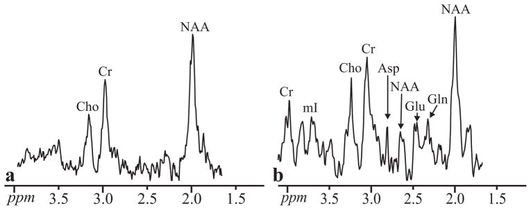
Magnified CSI-STEAM (a) and C-HSI (b) spectra from Fig. 5. The CSI-STEAM spectrum has been scaled ×2-fold to facilitate comparison with the C-HSI spectra. Note the presence of short T₂ metabolites (e.g. mI, Gln, Glu) in the C-HSI spectrum in contrast to the CSI spectrum.

In vivo Reproducibility

The area of the NAA, Cho and Cr lines was integrated for every voxel in each of the four back-to-back experiments. Their mean and standard deviation were then used to estimate their coefficient of variation (CV= standard deviation / mean) in each of the 256 voxels. The CVs’ distributions are shown in Fig. 7. The 15, 25 and 20% average CVs for NAA, Cr and Cho are in line with those reported for MRSI in voxels of this size at 3 T (36,37). The localizer scans performed between each of the back-to-back scans showed less than 3 mm subject motion.

Fig. 7.

Box plots showing the first, second (median), third quartiles (box), ±95% (whiskers) and outliers (+) of the coefficient of variation for the three major metabolites in the VOI. Note the concordance of these CVs with those reported in the literature for 3 T MRSI (36).

SAR

The SAR impact of the 90°_x – 180°_y – 90°_x C-HSI pulse combination was compared to that of a single, non-adiabatic, 13.5 ms, 180° pulse synthesized using optimal control methods (38,39) with 4 kHz bandwidth and 1 kHz peak B₁. The ratio of energy required to excite a single slice using the C-HSI pulse compared to that of the optimal control pulse was 20%. Since the same 0.5 ms, 2 kHz bandwidth 180° pulse is used to refocus multiple slices in the C-HSI pulse, this ratio is reduced further at higher resolutions, diminishing to 11% for the ×8 resolution.

Discussion

MRSI benefits from the increased sensitivity and spectral resolution offered by higher fields (14). However, increased chemical shift dispersion, together with lower available peak B₁, also exacerbate the CSD. The effect in 3D can be substantial: a small, 10%, CSD per spatial direction results in merely 73% overlap between two volumes (3). While Hadamard-encoding has been shown to offer better SNR and less bleed than conventional STEAM CSI (6,7), it is susceptible to CSD, especially at higher fields. The adiabatic pulses used in previous L-HSI applications (7,15) to overcome this, entail costs in SAR (since they have a higher time-bandwidth product), pulse length (T₂ losses) and bandwidth i.e., higher CSD, making them less suitable for higher fields than the sincs used here.

Indeed, our C-HSI pulses required a fraction of the energy of an optimized, non-adiabatic, inversion pulse per unit of excitation bandwidth, since the inversion 180° hard pulse is shared by all slices: C-HSI requires 2×N 90° selective pulses and a single 180° hard pulse to invert N slices. Had each slice been inverted independently, a total of N slice-selective 180° pulses would have been required. SLR-designed 180° pulses with the same bandwidth of a 90° pulse require approximately four-fold higher peak B₁ and an eight-fold higher SAR, implying that inverting the slices using N selective 180° pulses would require a four-fold increase in SAR compared to the 2×N 90° pulses (where we have ignored the hard 180° pulse’s negligible contribution). In fact, as long as the hard 180° inverts the desired spectral range, the CSD is determined by the 90° pulses and is, therefore, superior to the bandwidth achieved by a simple slice-selective 180° with the same peak B₁. Therefore, for a fixed SAR and peak B₁, significantly higher bandwidths and consequently, reduced CSDs, can be attained with C-HSI than either T-HSI or L-HSI.

In this paper we test the hypothesis that the SNR and localization advantages of HSI over CSI using identical acquisition parameters (FOV, voxel size and acquisition time) can be maintained at higher fields. Our findings, (Table 2 and Fig. 3), support this hypothesis. Specifically:

Localization

The C-HSI sequence’s voxel bleed in one dimension in the phantom, shown in Table 2, is 8–16% smaller than CSI’s, indicating better localization. This difference is apparent in Fig. 3 where the CSI bleed extends across the entire FOV (Fig. 3b) in contrast to the C-HSI bleed (Fig. 3c) which is smaller and more limited in extent. It should be noted that although the phantom’s 3 mm partition walls help reduce the bleed, since the voxels sizes are the same, both sequences benefit equally. The low bleed of C-HSI is also reflected by the minimal lipid peaks in the 1 – 2 ppm region of the spectra in Fig. 4. The apodized sincs used in C-HSI are simple to generate and provide improved localization over CSI despite being less than optimal.

B₁ inhomogeneity

As mentioned above, the 90°_x-180°_y-90_x° cascade inversion pulses offer greater resistance to B₁ variations compared to the 90°_x-180°_y-90_−x° non-inversion pulses. In the presence of large B₁ inhomogeneity, this difference may lead to unequal magnetization between the inversion and non-inversion pulses, potentially increasing voxel bleed. Due to the destructive-interference property of the Hadamard transform (40), this discrepancy leads only to a loss in SNR, not localization. Moreover, given the typical range of B₁ deviations in volume coils at 3T (41), these longitudinal magnetization values differences (obtained by simulation of the pulses in the presence of B₁ inhomogeneity) are under 10%. Finally, since the overall bleed for our sequence is smaller than CSI’s (shown in Table 2 and Fig. 3), its contribution to the total bleed is small. Note that since this effect is system-dependent it may be less apparent on a different instrument.

SNR

Peak B₁, pulse bandwidth and finite T₂ limitations yielded slice profiles that deviated from ideal rectangles by ~7%, as determined from the simulations. The calculated C-HSI bleed was based on the observed, 7% reduced signal. Accounting for both sources, i.e., slice profile imperfections and bleed, results in a 12–16% signal loss in the phantom compared to the ideal boxcar voxel shape. The ratio of the remaining signal in the two sequences (84–88% in C-HSI; 78–82% in CSI) predicts 1–12% SNR gain for C-HSI, in line with the results of Table 2.

CSD

Because it uses only gradient phase encoding for spatial localization, CSI is not subject to CSD. Nevertheless, to avoid outer volume contamination, it is used with selective VOI excitation, e.g., STEAM or PRESS that suffer from CSD, that can easily reach 2 mm/ppm in STEAM and 10 mm/ppm in PRESS (42). The 9 mT/m C-HSI selective excitation gradients used here, induce only 0.3 mm/ppm CSD, ×6 – ×35 fold lower than suffered by PRESS- or STEAM-CSI (42). (Although in PRESS or STEAM it only appears in voxels on the VOI edges, it is present in every voxel in C-HSI). This smaller CSD is coupled with the higher SNR, lower bleed and an ability to excite non-contiguous slices that are specific advantages of C-HSI.

Eddy Currents Immunity

The strong gradients used in the two sequences for selection and dephasing give rise to eddy currents. In contrast to CSI, the alternating gradients used for slice selection in C-HSI cause a cancellation of the eddy currents (43,44). Indeed, this effect is readily apparent in Fig. 3 where the linewidth of the CSI spectra is noticeably wider than that of C-HSI despite the fact that both experiments were performed back-to-back using the identical shim parameters.

In Vivo spectra

The sequential excitation of the slices resulted in TE ranging from 17 to 24 ms. These permit visualization of the short T₂ metabolites shown in Fig. 4, e.g. glutamine, glutamate, myo-inositol and aspartate. The absence of these metabolites in the in vivo CSI spectra in Figs. 5 and 6, demonstrate the increased SNR of our method. The reproducibility of the proposed sequence is similar to that obtained with CSI based methodology as well as superposition-based transverse Hadamard encoding at 1.5 T (6,36).

An N-th order longitudinal Hadamard encoding only yields N-1 “usable” slices since one is convolved with extraneous signals and typically needs to be discarded, leading to reduced coverage [p. 280 of (16)]. In the proposed sequence, the OVS scheme used effectively eliminates any extraneous signal thus avoiding this loss, as demonstrated by the 64 useable spectra in Fig. 4.

Post processing of J-coupled metabolites

The first-order phase shift caused by the slice-dependent variable TE of our sequence requires consideration in post-processing. Unlike the major singlets, J-coupled species and overlapping resonances cannot be simply corrected by a first-order phase correction. However, given the range of TE times in our sequence (17–24 ms) and the 1–10 Hz J-coupling of common brain metabolites, the resulting J-coupling induced phase shifts are small (since TE·J«1). Furthermore, regardless of the amount of shift, fitting each slice individually using a suitably generated basis set with the appropriate TEs (different basis set for each slice) (45) will account for both the J-coupling induced as well as the first order phase shifts.

Clinical Applications

The SNR and localization benefits of C-HSI that were demonstrated at large (8×8×4) grid size are enhanced further at smaller (×2, ×4) grids due to the reduced T₂ losses. This feature is particularly advantageous in the study of small brain structures like the anterior cingulate which plays a significant role in the study of Schizophrenia (46). Similar grid sizes used with CSI, would entail unmanageable inter-voxel bleed whereas C-HSI’s PSF remains close to ideal.

Limitations

Each slice tipped to the transverse plane undergoes a different T₂ weighting, depending on its order in the cascade. Depending on the length or number of pulses used and the metabolites T₂’s this decay can be non-negligible. Moreover, since the same cascade is also used in the second dimension, the losses are multiplicative. However, in light of the ~22 ms worst-case duration of the ×8 cascade block and given the ~300 ms (47) common T₂s for the major metabolites, the losses add up to ~13%. This sequence is nevertheless best suited for small (×2, ×4) grids or with short pulse elements. Additionally, while the CSD for PRESS or STEAM appears only in voxels at the VOI edges, in C-HSI it is present in every voxel, although it is mitigated by the much smaller CSD of C-HSI. Since the Hadamard reconstruction relies on linear combinations of the acquired FIDs, it is theoretically susceptible to patient motion. In our experience, however, motion has not been a significant problem both because the head is generally minimally affected by respiratory motion and because it is typically immobilized in the coil which has been shown to effectively reduce motion (48). The motion measured in in vivo scans was under 3 mm, as described in previous sections. As the VOI is made smaller, the corner volumes (shown in Fig. 4) become larger and hence may require stronger suppression to avoid VOI contamination. This may be achieved by optimization of the OVS pulses. Finally, the four step OVS phase cycling scheme determines the minimum scan time. Since the low SNR associated with MRSI often dictates multiple averages, this increase is acceptable for the typical MRSI resolutions in vivo.

Conclusion

The extraneous signal rejection achieved by the selective pulses, combined with destructive interference in the inverse Hadamard transform and the OVS scheme, are sufficient for short-echo acquisition, minimizing T₂ losses and J-modulations. With the ~15 minutes for subject-loading, shimming and MRI, the protocol requires less that ¾ hour, which can be tolerated by most. The RF waveforms used can be implemented on any modern imager and are safe with respect to their SAR. A near elimination of the chemical shift displacement, improved SNR and localization lend this method to clinical use, especially for small localization matrices.

References

- 1.Brown TR, Kincaid BM, Ugurbil K. NMR chemical shift imaging in three dimensions. Proc Natl Acad Sci U S A. 1982;79(11):3523–3526. doi: 10.1073/pnas.79.11.3523. [DOI] [PMC free article] [PubMed] [Google Scholar]
- 2.Maudsley AA, Hilal SK, Perman WH, Simon HE. Spatially resolved high resolution spectroscopy by “four dimensional” NMR. J Magn Reson. 1983;51:147–152. [Google Scholar]
- 3.Brown T. Practical applications of chemical shift imaging. NMR Biomed. 1992;5(5):238–243. doi: 10.1002/nbm.1940050508. [DOI] [PubMed] [Google Scholar]
- 4.Mareci T, Brooker H. Essential considerations for spectral localization using indirect gradient encoding of spatial information. J Magn Reson. 1991;92:229–246. [Google Scholar]
- 5.Wang Z, Bolinger L, Subramanian VH, Leigh JS. Errors of Fourier chemical shift imaging and their corrections. J Magn Reson. 1991;92:64–72. [Google Scholar]
- 6.Cohen O, Tal A, Goelman G, Gonen O. Non-spin-echo 3D transverse hadamard encoded proton spectroscopic imaging in the human brain. Magn Reson Med. 2012 doi: 10.1002/mrm.24464. [DOI] [PMC free article] [PubMed] [Google Scholar]
- 7.Tal A, Goelman G, Gonen O. In vivo free induction decay based 3D multivoxel longitudinal hadamard spectroscopic imaging in the human brain at 3 T. Magn Reson Med. 2013;69(4):903–911. doi: 10.1002/mrm.24327. [DOI] [PMC free article] [PubMed] [Google Scholar]
- 8.Goelman G, Liu S, Gonen O. Reducing voxel bleed in Hadamard-encoded MRI and MRS. Magn Reson Med. 2006;55(6):1460–1465. doi: 10.1002/mrm.20903. [DOI] [PubMed] [Google Scholar]
- 9.Young R, Serrai H. Implementation of three-dimensional wavelet encoding spectroscopic imaging: in vivo application and method comparison. Magn Reson Med. 2009;61(1):6–15. doi: 10.1002/mrm.21756. [DOI] [PubMed] [Google Scholar]
- 10.Tran TK, Vigneron DB, Sailasuta N, Tropp J, Le Roux P, Kurhanewicz J, Nelson S, Hurd R. Very selective suppression pulses for clinical MRSI studies of brain and prostate cancer. Magn Reson Med. 2000;43(1):23–33. doi: 10.1002/(sici)1522-2594(200001)43:1<23::aid-mrm4>3.0.co;2-e. [DOI] [PubMed] [Google Scholar]
- 11.Goelman G, Subramanian VH, Leigh JS. Transverse Hadamard spectroscopic imaging technique. Journal of Magnetic Resonance (1969) 1990;89(3):437–454. [Google Scholar]
- 12.Goelman G, Leigh JS. B1-insensitive Hadamard spectroscopic imaging technique. J Magn Reson. 1991;91:93–101. doi: 10.1002/mrm.1910250214. [DOI] [PubMed] [Google Scholar]
- 13.Goelman G, Liu S, Fleysher R, Fleysher L, Grossman RI, Gonen O. Chemical-shift artifact reduction in Hadamard-encoded MR spectroscopic imaging at high (3T and 7T) magnetic fields. Magn Reson Med. 2007;58(1):167–173. doi: 10.1002/mrm.21251. [DOI] [PubMed] [Google Scholar]
- 14.Vaughan JT, Garwood M, Collins CM, Liu W, DelaBarre L, Adriany G, Andersen P, Merkle H, Goebel R, Smith MB, Ugurbil K. 7T vs. 4T: RF power, homogeneity, and signal-to-noise comparison in head images. Magn Reson Med. 2001;46(1):24–30. doi: 10.1002/mrm.1156. [DOI] [PubMed] [Google Scholar]
- 15.Goelman G. Two methods for peak RF power minimization of multiple inversion-band pulses. Magn Reson Med. 1997;37(5):658–665. doi: 10.1002/mrm.1910370506. [DOI] [PubMed] [Google Scholar]
- 16.de Graaf RA. in vivo NMR Spectroscopy. Chichester, England: John Weily & Sons; 2007. p. 570. [Google Scholar]
- 17.Gonen O, Arias-Mendoza F, Goelman G. 3D localized in vivo 1H spectroscopy of human brain by using a hybrid of 1D-Hadamard with 2D-chemical shift imaging. Magn Reson Med. 1997;37(5):644–650. doi: 10.1002/mrm.1910370503. [DOI] [PubMed] [Google Scholar]
- 18.Levitt HM, Freeman R. NMR population inversion using a composite pulse. J Magn Reson. 1979;33:473–476. doi: 10.1016/j.jmr.2011.08.016. [DOI] [PubMed] [Google Scholar]
- 19.Levitt MH. Composite pulses. Prog NMR Spec. 1986;18:61–122. [Google Scholar]
- 20.Shinnar M. Reduced power selective excitation radio frequency pulses. Magn Reson Med. 1994;32(5):658–660. doi: 10.1002/mrm.1910320516. [DOI] [PubMed] [Google Scholar]
- 21.Matson GB. An integrated program for amplitude modulated RF pulse generation and re-mapping with shaped gradients. Magn Reson Imag. 1994;12:1205–1225. doi: 10.1016/0730-725x(94)90086-7. [DOI] [PubMed] [Google Scholar]
- 22.Bottomley PA. Spatial localization in NMR spectroscopy in vivo. Ann N Y Acad Sci. 1987;508:333–348. doi: 10.1111/j.1749-6632.1987.tb32915.x. [DOI] [PubMed] [Google Scholar]
- 23.Haase A, Frahm J, Hanicke W, Matthaei D. 1H NMR chemical shift selective (CHESS) imaging. Phys Med Biol. 1985;30(4):341–344. doi: 10.1088/0031-9155/30/4/008. [DOI] [PubMed] [Google Scholar]
- 24.Ebel A, Govindaraju V, Maudsley AA. Comparison of inversion recovery preparation schemes for lipid suppression in 1H MRSI of human brain. Magn Reson Med. 2003;49(5):903–908. doi: 10.1002/mrm.10444. [DOI] [PubMed] [Google Scholar]
- 25.Brief EE, Whittall KP, Li DK, MacKay A. Proton T1 relaxation times of cerebral metabolites differ within and between regions of normal human brain. NMR Biomed. 2003;16(8):503–509. doi: 10.1002/nbm.857. [DOI] [PubMed] [Google Scholar]
- 26.Ethofer T, Mader I, Seeger U, Helms G, Erb M, Grodd W, Ludolph A, Klose U. Comparison of longitudinal metabolite relaxation times in different regions of the human brain at 1. 5 and 3 Tesla. Magn Reson Med. 2003;50(6):1296–1301. doi: 10.1002/mrm.10640. [DOI] [PubMed] [Google Scholar]
- 27.Burger C, Buchli R, McKinnon G, Meier D, Boesiger P. The impact of the ISIS experiment order on spatial contamination. Magn Reson Med. 1992;26(2):218–230. doi: 10.1002/mrm.1910260204. [DOI] [PubMed] [Google Scholar]
- 28.Goelman G, Liu S, Hess D, Gonen O. Optimizing the efficiency of high-field multivoxel spectroscopic imaging by multiplexing in space and time. Magn Reson Med. 2006;56(1):34–40. doi: 10.1002/mrm.20942. [DOI] [PubMed] [Google Scholar]
- 29.Marion D, Ikura M, Bax A. Improved solvent suppression in one- and two-dimensional NMR spectra by convolution of time domain data. J Magn Reson. 1989;84(2):425–430. [Google Scholar]
- 30.Gonen O, Hu J, Stoyanova R, Leigh JS, Goelman G, Brown TR. Hybrid three dimensional (1D-Hadamard, 2D-chemical shift imaging) phosphorus localized spectroscopy of phantom and human brain. Magn Reson Med. 1995;33(3):300–308. doi: 10.1002/mrm.1910330304. [DOI] [PubMed] [Google Scholar]
- 31.Tal A, Gonen O. Localization errors in MR spectroscopic imaging due to the drift of the main magnetic field and their correction. Magn Reson Med. 2012;70:895–904. doi: 10.1002/mrm.24536. [DOI] [PMC free article] [PubMed] [Google Scholar]
- 32.Ernst RR, Bodenhausen G, Wokaun A. The International Series of Monographs on Chemistry. Vol. 152 Oxford: Clarendon Press; 1987. Principles of Nuclear Magnetic Resonance in One and Two Dimensions. [Google Scholar]
- 33.Maudsley AA. Sensitivity in Fourier Imaging. Journal of Magnetic Resonance. 1986;68:363–366. [Google Scholar]
- 34.Frahm J, Merboldt KD, Hanicke W. Localized proton spectroscopy using stimulated echoes. Journal of Magnetic Resonance. 1987;72:502–508. doi: 10.1002/mrm.1910170113. [DOI] [PubMed] [Google Scholar]
- 35.Duyn JH, Gillen J, Sobering G, van Zijl PC, Moonen CT. Multisection proton MR spectroscopic imaging of the brain. Radiology. 1993;188(1):277–282. doi: 10.1148/radiology.188.1.8511313. [DOI] [PubMed] [Google Scholar]
- 36.Kirov I, George IC, Jayawickrama N, Babb JS, Perry NN, Gonen O. Longitudinal inter- and intra-individual human brain metabolic quantification over 3 years with proton MR spectroscopy at 3 T. Mag Reson Med. 2012;67(1):27–33. doi: 10.1002/mrm.23001. [DOI] [PMC free article] [PubMed] [Google Scholar]
- 37.Wijnen JP, van Asten JJ, Klomp DW, Sjobakk TE, Gribbestad IS, Scheenen TW, Heerschap A. Short echo time 1H MRSI of the human brain at 3T with adiabatic slice-selective refocusing pulses; reproducibility and variance in a dual center setting. J Magn Reson Imaging. 2010;31(1):61–70. doi: 10.1002/jmri.21999. [DOI] [PubMed] [Google Scholar]
- 38.Conolly S, Nishimura D, Macovski A. Optimal control solutions to the magnetic resonance selective excitation problem. IEEE Trans Med Imaging. 1986;5(2):106–115. doi: 10.1109/TMI.1986.4307754. [DOI] [PubMed] [Google Scholar]
- 39.Khaneja N, Reiss T, Kehlet C, Schulte-Herbruggen T, Glaser SJ. Optimal control of coupled spin dynamics: design of NMR pulse sequences by gradient ascent algorithms. J Magn Reson. 2005;172(2):296–305. doi: 10.1016/j.jmr.2004.11.004. [DOI] [PubMed] [Google Scholar]
- 40.Gonen O, Murdoch JB, Stoyanova R, Goelman G. 3D multivoxel proton spectroscopy of human brain using a hybrid of 8th-order Hadamard encoding with 2D chemical shift imaging. Magn Reson Med. 1998;39(1):34–40. doi: 10.1002/mrm.1910390108. [DOI] [PubMed] [Google Scholar]
- 41.Jin J, Chen J. On the SAR and field inhomogeneity of birdcage coils loaded with the human head. Magn Reson Med. 1997;38(6):953–963. doi: 10.1002/mrm.1910380615. [DOI] [PubMed] [Google Scholar]
- 42.Scheenen TW, Klomp DW, Wijnen JP, Heerschap A. Short echo time 1H-MRSI of the human brain at 3T with minimal chemical shift displacement errors using adiabatic refocusing pulses. Magn Reson Med. 2008;59(1):1–6. doi: 10.1002/mrm.21302. [DOI] [PubMed] [Google Scholar]
- 43.Boesch C, Gruetter R, Martin E. Temporal and spatial analysis of fields generated by eddy currents in superconducting magnets: optimization of corrections and quantitative characterization of magnet/gradient systems. Magn Reson Med. 1991;20(2):268–284. doi: 10.1002/mrm.1910200209. [DOI] [PubMed] [Google Scholar]
- 44.Reese TG, Heid O, Weisskoff RM, Wedeen VJ. Reduction of eddy-current-induced distortion in diffusion MRI using a twice-refocused spin echo. Magn Reson Med. 2003;49(1):177–182. doi: 10.1002/mrm.10308. [DOI] [PubMed] [Google Scholar]
- 45.Soher BJ, Young K, Govindaraju V, Maudsley AA. Automated spectral analysis III: application to in vivo proton MR spectroscopy and spectroscopic imaging. Magn Reson Med. 1998;40(6):822–831. doi: 10.1002/mrm.1910400607. [DOI] [PubMed] [Google Scholar]
- 46.Hardy CJ, Tal A, Babb JS, Perry NN, Messinger JW, Antonius D, Malaspina D, Gonen O. Multivoxel Proton MR Spectroscopy Used to Distinguish Anterior Cingulate Metabolic Abnormalities in Patients with Schizophrenia. Radiology. 2011;147(2):362–367. doi: 10.1148/radiol.11110675. [DOI] [PMC free article] [PubMed] [Google Scholar]
- 47.Mlynarik V, Gruber S, Moser E. Proton T (1) and T (2) relaxation times of human brain metabolites at 3 Tesla. NMR Biomed. 2001;14(5):325–331. doi: 10.1002/nbm.713. [DOI] [PubMed] [Google Scholar]
- 48.Green MV, Seidel J, Stein SD, Tedder TE, Kempner KM, Kertzman C, Zeffiro TA. Head movement in normal subjects during simulated PET brain imaging with and without head restraint. Journal of Nuclear Medicine. 1994;35(9):1538–1546. [PubMed] [Google Scholar]