Spatio-Temporal Information Analysis of Event-Related BOLD Responses

Abstract

A new approach for analysis of event related fMRI (BOLD) signals is proposed. The technique is based on measures from information theory and is used both for spatial localization of task related activity, as well as for extracting temporal information regarding the task dependent propagation of activation across different brain regions. This approach enables whole brain visualization of voxels (areas) most involved in coding of a specific task condition, the time at which they are most informative about the condition, as well as their average amplitude at that preferred time. The approach does not require prior assumptions about the shape of the hemodynamic response function (HRF), nor about linear relations between BOLD response and presented stimuli (or task conditions). We show that relative delays between different brain regions can also be computed without prior knowledge of the experimental design, suggesting a general method that could be applied for analysis of differential time delays that occur during natural, uncontrolled conditions. Here we analyze BOLD signals recorded during performance of a motor learning task. We show that during motor learning, the BOLD response of unimodal motor cortical areas precedes the response in higher-order multimodal association areas, including posterior parietal cortex. Brain areas found to be associated with reduced activity during motor learning, predominantly in prefrontal brain regions, are informative about the task typically at significantly later times.

Introduction

Functional mapping is rapidly becoming a crucial tool for understanding principles of information representation and functional organization of the human brain. In particular, the noninvasive Functional Magnetic Resonance Imaging (fMRI) technique has been extensively used to identify functional areas and subdivisions in the human cortex.

The increasing popularity of using fMRI results in large data sets, which are usually analyzed in conventional ways. The conventional approach for the statistical analysis of Blood Oxygenation Level Dependent (BOLD) signals from fMRI is based on the general linear model [Friston et al., 1995; Worsley and Friston, 1995; Boynton et al., 1996].

According to the GLM, the signals can be represented as a linear combination of a set of model functions plus noise [Buxton, 2002]. The analysis consists of finding the set of amplitudes that scale each model function, to provide the best fit of the model in a least-squares sense (minimizing the sum of squares of the residuals after the estimated signal from the model is subtracted from the data). These sets of amplitudes are free parameters of the model, however the model functions are assumed to have a fixed shape.

Therefore, the first step in the GLM analysis is to predict the shape of the BOLD hemodynamic response to a given stimulus pattern. The hemodynamic response function (HRF) to a brief stimulus is assumed to be of a fixed shape [Henson et al., 2002], and the response to any other stimulus is modeled as a linear convolution of the HRF with the stimulus pattern.

While this powerful approach has without a doubt proven to be a useful framework for the study of functional brain organization, mainly in terms of the spatial localization of statistically significant task-related activity, the model is based on two fundamental assumptions, both of which are questionable under certain conditions.

First, the assumption of a constant HRF is problematic. HRF shapes have actually been shown to vary across regions, subjects and even cortical layers [Aguirre et al., 1998; Silva and Koretsky, 2002; Handwerker et al., 2004]. These findings have important consequences for the localization of task-related activated voxels. In fact, theoretically, localization could be so dependent on the HRF employed that by using different shaped HRFs, different brain regions could be highlighted, and determined to be “statistically significantly” activated (for experimental support see for example [Solbakk, 2005]).

The second questionable assumption is that of a linear relation between a given stimulus and the corresponding BOLD response. In fact, it has been shown that for sustained stimuli, the response is actually a sub-linear function of the stimulus duration [Boynton et al., 1996; Friston et al., 1998].

Moreover, even though the linearity assumption has proven to be a good approximation in many cases [Boynton et al., 1996; Dale and Buckner, 1997], mainly for long inter-trial intervals (ITI) between stimuli and for stimuli of relatively long duration (>4s), this may not be the case for other paradigms including short ITIs (<4s) or short stimuli (<3–4s) [Friston et al., 1998; Vazquez and Noll, 1998; Glover, 1999; Huettel and McCarthy, 2000; Liu and Gao, 2000].

The approach suggested in this study for the analysis of BOLD signals is a model-free one, thus no assumptions about the shape of the HRF for localization of task-related activity are required, and therefore it could account in theory for each voxel in the brain having its own pattern of response. Furthermore, this approach does not make any assumptions of linearity between the stimulus and BOLD response, and thus could be generalized for the analysis of sustained stimuli or short ITIs.

A further advantage of this approach is its ability to extract temporal information about the dynamics of brain activations. Temporal information regarding brain activations during task performance is crucial for our understanding of network interactions and functional connectivity between different brain regions. While spatial localization of task-related BOLD responses has been extensively explored for many task conditions, few studies only have addressed temporal aspects of neuronal circuitry engaged in task-performance. Despite the challenges in mapping of BOLD responses to underlying neural responses, several attempts have been made to address temporal aspects of BOLD responses, most within the framework of the GLM analysis [Menon et al., 1998; Menon and Kim, 1999; Miezin et al., 2000; Weilke et al., 2001; Formisano et al., 2002; Henson et al., 2002; Hernandez et al., 2002; Liao et al., 2002; Bellgowan et al., 2003; Mohamed et al., 2003; Saad et al., 2003; Sun et al., 2005]; see [Formisano and Goebel, 2003] for review). Some studies have used non-linear approaches for fitting the HRF [Calhoun et al., 2000; Richter et al., 2000]. Nevertheless, all these studies, excluding Sun and colleagues [Sun et al., 2005], assume a known shape of the HRF. However, it has been shown that latency analysis in particular is sensitive to the exact shape of the HRF in use [Hernandez et al., 2002; Handwerker et al., 2004].

Here we apply information theory for the analysis of fMRI data. In the past decade there has been an increasing interest in the application of information theory to various questions in neuroscience. Some examples include the study of single cell information coding in the fly [de Ruyter van Steveninck et al., 1997] and primate visual systems [Victor, 2000; Reich et al., 2001; Simoncelli and Olshausen, 2001; Kang et al., 2004], in the primary motor cortex [Paz et al., 2003], neural and population coding in general [Borst and Theunissen, 1999; Panzeri et al., 2003; Schneidman et al., 2003], as well as the study of cortical synaptic communication [Fuhrmann et al., 2002; Goldman et al., 2002]. However, to our knowledge, except for a few applications using ICA [McKeown et al., 1998; Arfanakis et al., 2000; Calhoun et al., 2000; Moritz et al., 2000] for cluster analysis, only one study has made an attempt to apply information theory for the analysis of fMRI time-series, by breaking the event-related responses into two epochs and computing the entropy at each half [de Araujo et al., 2003]. This analysis does not assume a constant shape of an HRF, but nevertheless assumes a general structure of signal with a maximal change at the first half of the event-related response. Moreover, only spatial localization of task-related activity is extracted. We propose a method to extract both spatial localization of task-related activity in the brain, as well as temporal information about the sequence of activation of different brain regions.

Information analysis is applied for studying spatio-temporal task-related activations during performance of a motor-learning task. Localized BOLD signal in cortical regions was measured while subjects performed a bimanual serial reaction-time task while learning a novel sequence. Spatial localization of task-related activity is compared to maps calculated using the standard GLM analysis, and is shown to involve a motor cortical network, as well as more prefrontal regions than those revealed by the GLM analysis. Temporal analysis is performed for single subjects as well as for the grand average of all subjects, and compared to latency analysis performed according to peak of event-related responses as well as according to the time of minimal variance in responses. Finally, sequential activation of specific regions of interest (ROIs) is performed by computing mutual information between pairs of ROIs, without using knowledge of the experimental design. The principal regions of interest in this study include the primary sensorimotor cortex (S1/M1), premotor cortex (PM), supplementary motor area (SMA), and posterior parietal cortex (PPC).

Materials and Methods

Experimental methods

Subjects and Behavioral Task

Data from fourteen right-handed subjects (4 female; ages 19–29 years; mean age = 23.5) from an existing data set [Sun et al., 2005] were analyzed for the purpose of this study. The original data set consists of fourteen subjects that participated after giving informed consent according to procedures approved by the University of California. The subjects reported no history of neurological or psychiatric disorders and were taking no medications at the time of the study.

Training

Prior to scanning, subjects were trained on one of two bimanual sequences; sequence A, denoted by L4-R2-L3-R4-L5-R5-L2-R3, or sequence B, denoted by L5-R3-L2-R5-L4-R2-L3-R4. Here, the letter signifies the hand (R=right, L=left) and the number signifies the finger (2=index finger, 3=middle finger, 4=ring finger, 5=fifth finger). During training, the subjects were seated comfortably in a dimly lit room. Each hand was positioned on a 5-fingered response box such that each finger aligned with a single key. The training sequence was presented to the subject as a series of visual cues indicating the key to press. The response window for each cue was 725 ms, and subjects were instructed to respond as quickly and accurately as possible upon seeing each cue. A sequence was considered correct only when all eight key presses were performed correctly. The same sequence was repeated 20 times within a set, with a 2 sec interval between each sequence. Subjects were trained until they were able to complete a set of sequences with an accuracy of at least 85%. Training sessions consisted of an average of 4 sets (80 sequence trials).

MRI Scanning

In the MRI scanner, five 8-minute functional runs were acquired for each subject using a mixed block/event-related paradigm [Visscher et al., 2003]. The runs were composed of 4 condition blocks (LEARN, PLAY, RANDOM, and FIXATION), each presented twice in a pseudo-random order, counter-balanced across subjects. Each block began with an instructional cue, indicating the type of block. Within each of the PLAY, LEARN, and RANDOM condition blocks, sequences were presented with visual cues as in training (725 ms/key press, 5800 ms/sequence), but with a pseudo-randomized inter-trial interval (ITI) of 2.2, 4.4, or 6.6 seconds (Figure 1). During the PLAY condition, subjects were presented with the same sequence that they learned during the training session (e.g. Sequence A). During the LEARN condition, subjects were presented with the alternate sequence (e.g. Sequence B), which was novel to them at the beginning of the scan session. Subjects were instructed to learn the sequence across the blocks. During the RANDOM condition, subjects were presented with a new sequence for each trial. Subjects were instructed to play all sequences as accurately as possible. Five sequences were presented in each block for a total block length of 58 seconds. During the FIXATION block, also of length 58 seconds, subjects were presented with a centered fixation cross. For this condition, subjects were instructed not to perform or rehearse any of the sequences. Subjects received accuracy and timing information at the conclusion of each condition block. The results from the LEARN condition are presented in this paper. The stimuli were designed and presented using Eprime presentation software (www.pstnet.com). They were then back-projected onto a custom-designed, non-magnetic projection screen that the subject viewed via a mirror. Responses were collected using a pair of five-fingered MR-compatible keyboards.

Figure 1.

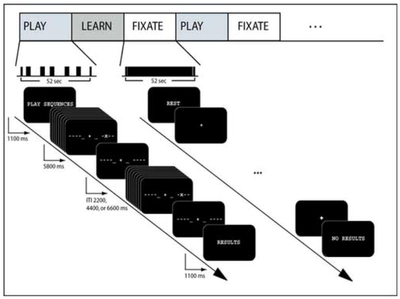
Experimental design.

MRI Data Acquisition

All images were acquired with a 4 Tesla Varian INOVA MR scanner (www.varianinc.com) and a TEM-send and receive RF head coil (www.mrinstruments.com). Functional images were acquired using a 2-shot gradient-echo echo-planar image (EPI) sequence with a repetition time (TR) of 543 ms per shot, with an echo time of 28 ms, and flip angle of 20°, resulting in 432 total volumes acquired per run (864 after time-interpolation). Each volume, covering the top of the brain, consisted of ten 5 mm thick axial slices with a 0.5 mm inter-slice gap. Each slice was acquired with a 22.4 cm² field of view with a 64 × 64 matrix size, resulting in an in-plane resolution of 3.5 × 3.5 mm. High resolution (.875 × .875 mm) in-plane T1-weighted anatomical images were also acquired using a gradient-echo multi-slice (GEMS) sequence for anatomical localization. Finally, MPFLASH 3D T1-weighted scans were acquired so that functional data could be normalized to the Montreal Neurological Institute (MNI) atlas space.

Methods of data analysis

Preprocessing

Functional images acquired from the MR scanner were reconstructed from k-space using a linear time-interpolation algorithm [Noll DC, 2000] to double the effective sampling rate, and corrected for slice-timing skew using temporal sinc-interpolation. Images were then corrected for movement using rigid-body transformation parameters, and smoothed with an 8 mm full width at half maximum (FWHM) Gaussian kernel using the software package SPM2 (www.fil.ion.ucl.ac.uk/spm).

Information theoretic analysis

Data analysis is based on concepts from information theory. In particular, we quantify the information contained in the BOLD signals of a voxel about a preceding task condition. To compute this information we use two information theoretic measures ([Cover and Thomas, 1991].

The first measure is the entropy of a random variable that quantifies the amount of uncertainty one has about its value. For a discrete random variable X, which can take any value x from a particular set χ with probability p(x), the entropy H(X) in bits is calculated as follows:

$$H(X)=-\sum _{x=\chi }p(x){log}_{2}p(x)$$ Equation 1

Generally, the wider the probability distribution of the possible values of X, the harder it is to guess the exact value of the variable at a given instance, and thus the entropy is larger. Relevant random variables for the present study are the magnitude of the BOLD signal of a voxel and the stimulus, or a code representing a task condition. The second information theoretic measure is the mutual information, I(X; Y), between a pair of random variables X, Y. It is defined using the conditional entropy of X given Y, H(X|Y):

$$\begin{array}{l}H(X\mid Y)=\sum _{y=y}p(y)H(X\mid Y=y)\\ =-\sum _{y=y}p(y)\sum _{x=\chi }p(x\mid Y=y){log}_{2}p(x\mid Y=y)\end{array}$$ Equation 2

where p(x|Y=y) is the conditional probability of X = x given the value y of Y. If X (e.g., the BOLD response) is statistically correlated to Y (e.g., the preceding stimulus), then knowledge of Y reduces the uncertainty about the value of X. In this case, H(X|Y) will be less than H(X), which we refer to as the unconditional entropy. This reduction in uncertainty about a single random variable X, due to the knowledge of another variable, is quantified by the mutual information and is given by the difference between the unconditional and conditional entropies of X,

$$I(X;Y)=H(X)-H(X\mid Y)$$ Equation 3

This measure is symmetric: I(X; Y) = I(Y; X), i.e., the information that a stimulus has about the BOLD response to follow is equal to the information that the response has about the preceding stimulus.

The entropy of a continuous random variable (as are the BOLD responses) is computed, in practice, by dividing the range of X into finite bins of a chosen precision (Δ) and evaluating the resulting probability distribution of the corresponding discrete variable. The computed entropy will therefore depend on the precise choice of the bin size:

$$H(X^{\mathrm{\Delta }})=-\sum \mathrm{\Delta }f(x_i)logf(x_i)-log\mathrm{\Delta }$$ Equation 4

where f(x_i) is the X’s density function.

However, it has been shown that as the bin size (Δ) approaches zero

$$H(X^{\mathrm{\Delta }})\to h(X)-log\mathrm{\Delta }$$ Equation 5

Therefore, if the bin size is sufficiently small and set constant for both conditional and unconditional entropies, then the computed mutual information I(X;Y) is independent of the bin size:

$$\begin{array}{l}I(X^{\mathrm{\Delta }};Y^{\mathrm{\Delta }})=H(X^{\mathrm{\Delta }})-H(X^{\mathrm{\Delta }}\mid Y^{\mathrm{\Delta }})\\ \approx h(X)-log\mathrm{\Delta }-(h(X\mid Y)-log\mathrm{\Delta })\\ =I(X;Y)\end{array}$$ Equation 6

where h(X) is the entropy of the continuous random variable X [Cover and Thomas, 1991].

Information analysis of BOLD responses: Localization of task-related activities

We use the measure of mutual information (Eq. 3) to quantify the reduction in uncertainty about the reference task condition (REF), which is achieved by knowing the magnitude of BOLD response at a fixed time delay (latency, dt) later. Latencies are chosen as multiples of TRs. All time series of BOLD signals are z-normalized to have zero mean and unit variance. If more than one scanning epoch is performed, the time series from each scanning epoch are z-normalized separately. Therefore, the analysis focuses on changes of responses relative to baseline activity.

To evaluate the unconditional entropy of responses, we start by estimating the probability distribution of all BOLD responses of a voxel that ever occurred anytime during the experiment (Fig. 2A,B top histograms). In a sense, temporal information is collapsed. To estimate the distributions, we break the responses into N_bins equally spaced bins. The conditional entropy of responses is computed similarly, by estimating the probability distributions of only those responses that followed all the instances of the chosen (e.g. LEARN) condition, after a fixed time delay (dt) (Fig. 2A,B middle histograms) and in the same way, the responses that follow any other task condition (Fig. 2A,B bottom histogram).

Figure 2.

A,B: Histograms of responses for the same voxel at 2 different considered time delays (latencies) between the task condition and the amplitude of the BOLD response. A. (Left): at the estimated preferred latency of this voxel (3.258 s). B. (Right): at a different estimated latency (7.059s). For each of the latencies the top histogram is a histogram of all responses (LEARN + all other). Middle: histogram of responses that follow the chosen condition only (LEARN). C. (Bottom): histogram of responses that follow any other condition. C. Bottom curve: MI plotted as a function of the considered latency between a task condition and the response for the same voxel.

For most voxels, the histogram of responses following the chosen (LEARN) condition is very similar to the histogram of all responses. In fact, most of the voxels did not exhibit a clear difference between these two histograms.

However, some voxels, as the one depicted in Fig. 2A, do show a marked difference. In these voxels, the histogram of responses that follow the chosen condition is somewhat shifted to the right, meaning that larger BOLD responses at this voxel are more likely to follow the chosen condition. This reveals that increased responses code for the fact that the chosen condition was presented. Other voxels could code the specific condition as relatively decreased responses instead, and this would be evident from a conditional distribution, which is shifted to the left. In either case, as the two bottom distributions become more separable, it is easier to guess the preceding condition (LEARN/not-LEARN) simply by knowing the amplitude of response.

According to the a-priori distribution of all responses, regardless of the task condition preceding it, we compute the unconditional distribution of all responses. All responses include the responses to the chosen condition (LEARN) and the responses to all other conditions. Then, from all responses that specifically follow the chosen condition (LEARN) we can estimate the conditional distribution. The same is done for responses that follow the other conditions, and the unconditional entropy of responses is computed. The MI is computed as the difference between these two entropies.

$$I(\mathit{BOLD};\mathit{REF})=H(\mathit{BOLD})-H(\mathit{BOLD}\mid \mathit{REF})$$ Equation 7

i.e., the reduction in uncertainty about the preceding task condition, due to the knowledge of the magnitude of BOLD response.

The number of bins (N_bins) used to estimate the probability distributions was chosen to be 1000, after testing convergence of I (X ^Δ ;Y ^Δ) to I(X;Y) for different bin sizes (Δ, see Eq. 5 and 6). A bin size of 0.001 of the maximal amplitude of the response was small enough to reach convergence to I(X;Y).

Calculating MI for all voxels in the scanned volume of the brain, results in a higher value of MI for voxels that are informative about, or involved in coding the task condition, than for those that are not. For localization of task-related activity, we search for voxels that best code for the chosen task condition.

In addition, we note that the information content of a given voxel about the chosen condition depends on the considered latency (dt) between the task condition presentation and the BOLD response. For the voxel depicted in Fig 2, we show on the right (B) that for a non-optimal considered latency, the information content of the voxel about the task condition is reduced. Fig. 2C summarizes the dependence of the mutual information content of the same example voxel, for different considered time delays. It is apparent that the voxel has a preferred latency of response (at about 3s) for which information content is maximal.

MI of each voxel is therefore computed for different possible latencies (dt), and each voxel is attached with its maximal information at whatever latency. To account for a wide range of event-related BOLD responses, the range of possible dt was determined in increments of TR starting from one TR up to 17 TRs (9.231 s). Task-related (significantly informative) voxels are chosen as those with MI value (at the maximal point) that exceeds MI-significance threshold. In order to estimate MI-significance threshold we use the 15 voxels with the highest information content about the chosen condition, at whatever latency they occur. For each of these voxels (i) we compute the average MI value for 100 randomized permutations of the BOLD time series relative to the experimental reference function (MIⁱ_rand100). The MI-significance threshold (ϑ^MI_mean) is then set as the average of those values over the 15 voxels (<MIⁱ_rand100>_i=1:15). An alternative significance threshold (ϑ^MI_std), set as the mean plus one standard deviation of those values, is also computed and used to threshold the data. Unless stated otherwise, results are presented for information threshold ϑ^MI_mean.

Contrast maps for two active task conditions (A,B), analogous to GLM contrast maps, although not presented in this paper, may be obtained by computing for each voxel:

$$\mathrm{\Delta }{\text{I}}_{\text{A},\text{B}}=\text{I}(\text{BOLD};\text{A})-\text{I}(\text{BOLD};\text{B}).$$ Equation 8

ΔI_A,B >0 indicates that a voxel is preferentially coding the task B than task A, equivalent to being preferentially activated by task B in the GLM framework. In theory, each voxel may have a different preferred delay to either task condition, for example having shorter latency for A (dt_A) than for B (dt_B). Therefore, in the same way, a differential time lag Δdt_A,B = dt_A − dt_B can be computed, representing the difference in the latency of the most informative response to each of these conditions (>0 if the maximal information about B is obtained at a shorter latency than for A, and vice versa for <0).

We note, however, that ΔI_A,B ~= 0, in the case where a voxel has a similar information content about either task condition (A or B) doesn’t necessarily mean that the voxel cannot distinguish between A,B. (This is analogous, in the GLM framework, to voxels which are being activated to the same degree for both task conditions).

It could be that a voxel carries the same amount of information about the precedence of either of these tasks (with respect to any other tasks), but at the same time it has the capacity to distinguish between them. If this is the case, and one is searching for voxels that can best distinguish whether the preceding task condition was A or B, given that it was one of them, the following approach can be used. To estimate the unconditional distribution of responses (as the top in Fig. 2), one should take only responses that follow either of the task conditions (A,B). The responses to the condition A are responses that follow A by a certain dt_A, and the responses to B are the responses that follow B by dt_B. The conditional distributions (as the middle and bottom in Fig. 2) should each hold the responses to A (after dt_A), and the responses to B (after dt_B).

Therefore, in order to allow for each voxel to have a different preferred delay to each task condition, one should search for the maximal information content in a two dimensional surface of (dt_A, dt_B).

Preferred latency of task related voxels

We define the preferred latency of a voxel as the latency that maximizes the information contained in its BOLD response about a chosen task condition (see example in Fig. 2C). For each task-related voxel, we determine its preferred latency, as the time interval (dt) that maximizes information content of its responses about the chosen task condition. We construct whole brain latency maps, in which the color at each voxel indicates its preferred latency.

Assessing relative amplitudes of responses at the preferred latency

Since mutual information is not sensitive to whether there was an increase or decrease in the magnitude of response to the task condition, for each task-related voxel we determine what was its amplitude of response at its preferred latency. Specifically, we are interested in the latency in which the event-related response is maximally informative about the task condition, and whether the magnitude of response with which it was coding it is relatively increased or decreased.

Localization and preferred latency assessment by mean and variance of BOLD responses

As a complementary issue, task-related localization was performed in two other methods. According to the first, task related voxels are chosen as those in which a maximal change in amplitude (from baseline) is observed on average in response to the chosen condition. In other words, maximal average peak of event related responses. The change can be obtained at any latency, thus at different latencies for different voxels. In the same way, according to the second method, task-related voxels are chosen as those with minimal variance in the responses to the chosen condition. In both these methods, preferred latencies of chosen voxels are also determined, i.e. latencies which maximize average peak of event-related response, or minimize variance of responses. We will refer to these as the M-latency map and V-latency maps, respectively.

Studying sequence of activations of regions of interest (ROIs)

Finally, temporal sequence of activation of specific regions of interest (ROIs) is determined in the two following ways. According to the first, latency of an ROI is determined for each individual subject as the average latency in all voxels within the subject-specific ROI mask (in MNI space); then for each ROI the average ROI latency, as well as standard error, over all subjects is computed. According to the second way, latency of each ROI is computed directly from the grand average latency maps (computed as the average of individual subjects latency maps, each in MNI space), using grand average ROI masks (see below). Standard error in this case is computed across all voxels within the ROI. This is done for all three types of latency maps: information latency maps, M-latency maps, and V-latency maps.

Based on evidence in the literature and results from the univariate analysis we chose the ROIs within the primary sensorimotor cortex (S1/M1), premotor cortex (PM), supplementary motor area (SMA), and posterior parietal cortex (PPC). For each of the ROIs, anatomical masks were defined in the subjects’ native space. The S1/M1 mask included cortex adjacent to the central sulcus, extending anteriorly to the mid-line between the central and precentral sulcus, posteriorly to the mid-line between the central and post-central sulcus, and dorsally and ventrally to include the primary motor hand area [Yousry et al., 1997]. The dorsal PM mask extended from the mid-line between the central and precentral sulcus, anteriorly to the junction of the superior frontal sulcus and the precentral sulcus. To exclude ventral premotor regions, the PM mask included only cortex dorsal to the inferior frontal sulcus [Picard and Strick, 2001]. The SMA mask was located on the medial wall, dorsal to the cingulate gyrus, and between the central sulcus and the vertical plane through the anterior commisure (VAC) [Picard and Strick, 2001]. The PPC mask included cortex in the superior parietal lobe posterior to and inclusive of the post-central sulcus, and adjacent to the intra-parietal sulcus at the junction of the two sulci [Simon et al., 2002]. All masks were non-overlapping. For each ROI, grand average masks were defined as the union of all individual subjects’ masks in MNI space

In addition, an anatomical mask was also constructed for the prefrontal cortex. The mask included the dorsal half of the prefrontal cortex as defined in [Duvernoy, 1999]. On the anterolateral surface of the frontal cortex, the ROI mask extended posteriorly to the inferior frontal sulcus (IFrS), and dorsally to a line drawn between the anterior tip of the superior frontal sulcus and the intersection of the IFrS and the inferior precentral sulcus. Medially, the mask included portions of the superior and middle frontal gyri, extending posteriorly to the sulcus just anterior to the cingulate sulcus (this sulcus roughly marks the anterior border of BA 32). On the dorsal surface, the mask terminated posteriorly at the limit of BA 9.

Relative timing of information coding between pairs of ROIs, regardless of the experimental design

To address functional connectivity, regardless of any prior knowledge of the stimulus (reference function), instead of studying the relation between BOLD responses and the reference conditions, we now study the relation between the average BOLD responses of one specific ROI and the average BOLD response of another specific ROI.

To do so, one ROI is considered as the “stimulus” ROI (ROI₂) and we compute the reduction in uncertainty about the responses (magnitude of signals) in the other region (ROI₁), which is obtained by knowing how large the signal in ROI₂ was. In other words, we are testing whether having a relatively large ROI₂ signal would, for instance, suggest that a relatively small ROI₁ response would follow and that a small ROI₂ response would predict a large ROI₁ response. This would indicate that signals in one region are informative about the magnitude of the signal in the other region.

Instead of having just two conditions (LEARN;NON-LEARN), as in the voxel based information analysis, here we have a whole range of ROI₂ response magnitudes used to condition the ROI₁ responses upon. Therefore, the responses of ROI₂ are split into a small number of bins (typically 6, unless stated otherwise), according to their magnitudes (very small to very large). We then estimate the unconditional distribution of all ROI₁ responses, as well as the distributions conditioned on each of these 6 bins of ROI₂ responses.

The responses of ROI₁ are responses that follow or preceded those of ROI₂ by a certain latency dt. MI between the two ROIs is computed for both positive and negative values of dt.

The number of bins used to break up the ROI₂ data is set according to data size limitations, to allow the estimation of the distribution of the responses of ROI₁ conditioned on each of the ROI₂ bins. The bin size used to estimate the distributions of ROI₁ responses (conditioned and unconditioned) is 1000, as used for the voxel-based information analysis.

Note that the analysis is based on a stationarity assumption, according to which the same sequence of brain activations is observed throughout the analyzed time period (i.e. that one ROI is always responsive before the other).

A modified version of this analysis could also used to study condition-based relative timing, i.e the sequence of brain activations following a specific task condition (e.g. LEARN). In this case, the continuous time series for each of the 2 ROIs would be segmented into trials of certain epoch duration (typically ~10–15 s, depending on the relevant duration of the event-related response). The responses from all trials are collapsed together to estimate both the conditional and unconditional distributions. This approach also reduces the stationarity assumption to only the epoch, such that the sequence of ROI activations is only assumed to persist during the relatively short epoch. This analysis, however, naturally requires knowledge of the experimental design. Moreover, it requires the design of an experiment with a very large number of trials to allow the estimation of both unconditional ROI₁ responses, as well as ROI₂-conditioned ROI₁ responses, from those relatively short epochs.

For comparison, we also compute the simple linear correlation between the time-lagged time series from the two ROIs. This is done by computing the correlation coefficient between the time-shifted time series, with varying latencies.

Localization using GLM

For comparison of spatial localization results to standard GLM analysis we use SPM2. To model task-related activity, we used SPM’s canonical hemodynamic response function (HRF; [Josephs et al., 1997]) convolved with independent variables for the onset and duration of each sequence. Here, the duration of each sequence was modeled as an epoch of 5800 ms. These covariates were entered into the modified GLM for analysis.

Following the preprocessing stage (see above), parameter estimates, reflecting the percent signal change relative to baseline were estimated for each covariate. Statistical parametric maps (t-statistics) of contrasts were generated for individual subjects with significance values of p<.05, corrected (FWE). Brain activations were masked using SPM2.

Results

The proposed method of analysis was applied to data acquired from subjects performing a motor learning task.

Spatial analysis: Localization of Task-Related Activity

We perform whole-brain information analysis for the localization of brain activations that are related to learning of the motor task. Fig. 3A (top left) depicts an example of one brain slice of such a functional map, constructed for a single subject. Only voxels found to be significantly informative (MI> ϑ^MI_mean) about the LEARN condition are shown. Task-related activations were found mainly in the motor network, including the primary and premotor motor areas (M1, PM), supplementary motor areas (SMA and preSMA), as well as in the posterior-parietal cortex (PPC). These activation are in agreement with task-related activations reported in previous studies (see [Swinnen, 2002], [Willingham, 1998] for reviews) as well as with a functional map constructed using standard GLM analysis [Sun et al., 2005] for the same data set (Fig. 3B; p<0.05, FWE corrected).

Figure 3.

Spatial localization of task-related activity (subject 212). A. Using information analysis. Task-related voxels are highlighted in red-orange. Top left: ϑ^MI_mean · is used as threshold for significantly informative voxels. Top right: ϑ^MI_std threshold is used. Activations outside the brain are unmasked, and ghosting artifacts are observed. B. Using standard GLM analysis (contrast FIXATION, t-threshold 4.46). Activations outside the brain are masked. C. Using information analysis. For the comparison with GLM results, activations outside the brain are masked (same mask as in B) and threshold is determined to pick the same number of mostly informative voxels as determined by GLM (B).

An alternative significance threshold (ϑ^MI_std; see methods) was also tested (Fig. 3A top right). From comparison of the resulting functional maps to those created using GLM analysis (Fig. 3C), this threshold is conservative. Therefore, results in this paper are presented for ϑ^MI_mean.

To provide an accurate comparison between the MI and GLM localization, in terms of the spatial distribution of task related activity, we masked the subject’s MI-maps using the brain mask created by SPM (see methods for GLM localization), and picked the same number of the most informative voxels as chosen by GLM (Fig. 3D).

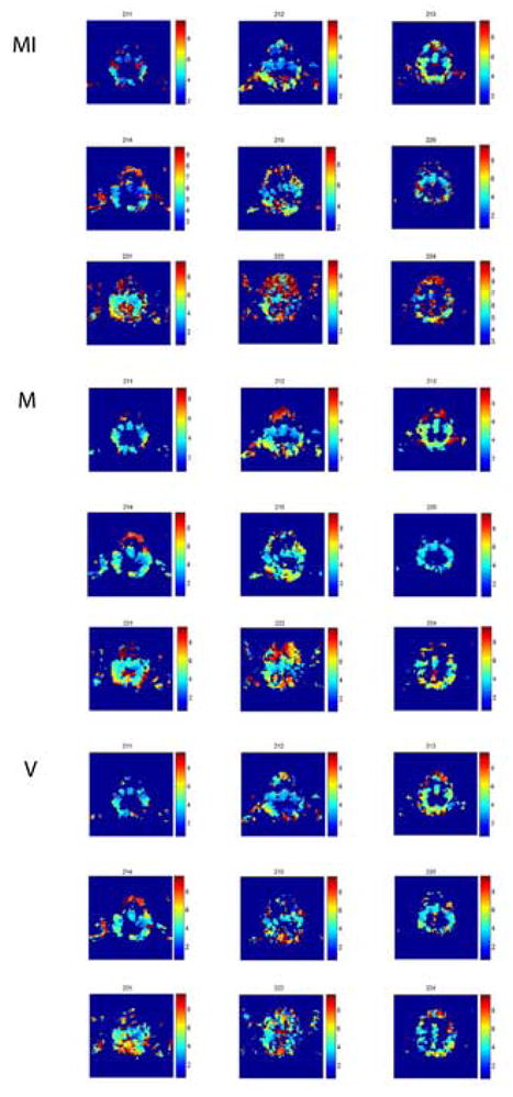
Note that as apparent in the presented slice (as well as highly evident in slices not shown), even with the most conservative threshold (ϑ^MI_std), information analysis localized task related activity in more extensive prefrontal regions, including areas that are not chosen to be task-related using the standard GLM analysis. Task-related activity in prefrontal regions was observed in most subjects (Fig. 5 top; as well as subjects not shown). This effect is summarized in Table 1.

Figure 5.

Comparison of spatial localization of task-related activity according to the 3 approaches (MI,M,V) for 9 representative subjects (Axes: Anterior-posterior: top-bottom). Top: MI value (at the preferred latency) for significantly informative voxels. Same brain slice is shown as in Fig. 3. Middle: M-value for the same number of voxels with highest M-values. Bottom: V-value for the same number of voxels with minimal V-values.

Table 1.

% Significant task related activation in the PFC

Subject	GLM	MI	M	V
209	2.69	18.65	1.67	11.55
211	3.33	10.58	5.17	11.00
212	16.46	42.02	9.31	7.84
213	4.34	41.62	6.47	4.85
214	2.08	4.49	5.74	11.39
215	3.26	14.68	5.91	15.36
219	0.18	2.68	0.00	10.01
218	0.26	19.38	5.33	2.12
220	2.58	10.42	4.54	4.90
221	0.19	9.79	0.67	2.98
222	1.29	10.00	3.79	3.53
223	0.00	2.75	0.00	0.47
224	0.00	27.44	1.81	6.33
225	3.22	27.03	2.62	1.74

Comparison of % task-related activation within the prefrontal cortex (PFC), according to GLM, MI, M, and V approaches for each of the subjects. Numbers represent the percent of significantly activated voxels within the PFC. This is computed after thresholding all activation maps (MI,M,V) such that the number of significantly activated voxels within the brain is matched to the number determined by the thresholded GLM t-map with p<0.05, FWE corrected (see also Fig. 3D).

To understand these effects, we studied the event-related responses of voxels in the regions of interest (Fig. 4). Fig. 4A depicts the canonical HRF, which is used in this study in order to model the hemodynamic response to the task reference function. The HRF represents the model response to a brief stimulus. The typical event-related responses in the motor regions (Fig. 4B) resemble the canonical HRF, with a clear amplitude peak of the event-related response around the same latency as the peak of the canonical HRF. These responses can therefore be modeled by the GLM, and voxels within those regions will be selected later on as being significantly activated. In contrast, the responses in the prefrontal cortex (Fig. 4C) seem to be less typical, commonly having double opposite-sign peaks (left), a shifted peak (~8–10 s or later; right), or even a state switch with no peak at all (middle). These responses could not be modeled correctly by the canonical HRF, and therefore these voxels are missed by the GLM analysis.

Figure 4.

Study of event-related responses. A. The canonical HRF used in order to model the hemodynamic response to the task reference function. The HRF represents the modeled response to a brief stimulus. B. Typical event-related BOLD responses (ERBs) to the LEARN condition resemble the canonical HRF. Examples from voxels in motor related regions. C. Event-related responses of voxels within the prefrontal cortex to the LEARN condition. ERBs are less typical, and do not resemble the canonical HRFs. (Left) The most abundant event-related response at prefrontal regions has a double peak (a negative followed by a positive peak), crossing zero signal change at a latency of around 6 seconds. (Middle) Non peaked state-switch responses. (Right) long latency peaked responses. All examples are taken from subject 212.

To test contrast maps between two active conditions, activation maps were also created for the contrast between the LEARN versus the PLAY condition (results not shown). In the group average data there was no statistical significant difference for the GLM map (p<0.05, FWE corrected, and a few supra-threshold voxels only for p<0.001 uncorrected). However, to test the underlying spatial distribution of differential activation, we also looked at the GLM contrast map for a liberal threshold (p<0.05, no correction) and compared it with the map created using the analogous information theory approach (see Methods, Eq. 8), using a significance threshold matched to yield the same number of significantly activated voxels. We found that the spatial distribution is similar using the two approaches, such that voxels which are preferentially activated, or coding, one of the two active conditions are found mainly in the motor network (PM, M1, SMA and PPC), with some distinctions between the two analysis approaches (e.g. more bilateral activation using the information theory approach, in return of several white matter blobs of activation using the GLM). We note that a third contrast map, created directly by computing the mutual information between the BOLD response and the preceding task condition where the only two considered conditions are the PLAY vs. LEARN (see Methods; using dt_A and dt_B), reveals the involvement of more association areas.

Temporal analysis: Preferred latency maps

To study the dynamics of event-related brain activations, latency maps are constructed. The information contained in the amplitude of the event-related response about the task condition which preceded it by a certain dt, is computed for all dt values ranging from one TR to 10s (in steps of TR). Each voxel is then assigned with its preferred latency, the latency for which the event related response of the voxel is most informative about the preceding task condition (see also Methods).

In Fig. 6 and Fig. 7B (same, with colorbar), latency map is presented for the significantly informative voxels for the same subjects as in Fig. 3. From this slice, it can be seen that task-related informative activity begins in the SMA, premotor and primary motor areas at about 3–4s after the chosen task condition, propagates to the PPC at about 5 s, and finally reaches lateral portions of the left PPC even as late as 7s after event initiation. Task-related activity of different voxels at prefrontal areas is informative about the task at a variety of latencies, some of which are as late as 8–9s after the beginning of the event. In Fig. 8A latency maps of 9 of the subjects are presented for the significantly informative voxels, and inter-subject similarities in the spatiotemporal distribution of informative responses can be observed. In all subjects, the preferred latencies of voxels within the SMA, premotor and primary motor regions (at about 3–4 s delay) are shorter than those of the higher association areas, mainly the PPC (at about 5–7s). In most subjects, the majority of voxels within the task-related voxels in prefrontal cortex respond significantly later (>8s).

Figure 6.

Slice of a preferred latency map as computed for a single subject (same subject as in Fig. 3). Preferred latencies the task-related voxels are color coded and overlaid on the subject’s brain. Scale of colors from blue to red indicates short to longer latencies (for quantitative scale see Fig. 7B).

Figure 7.

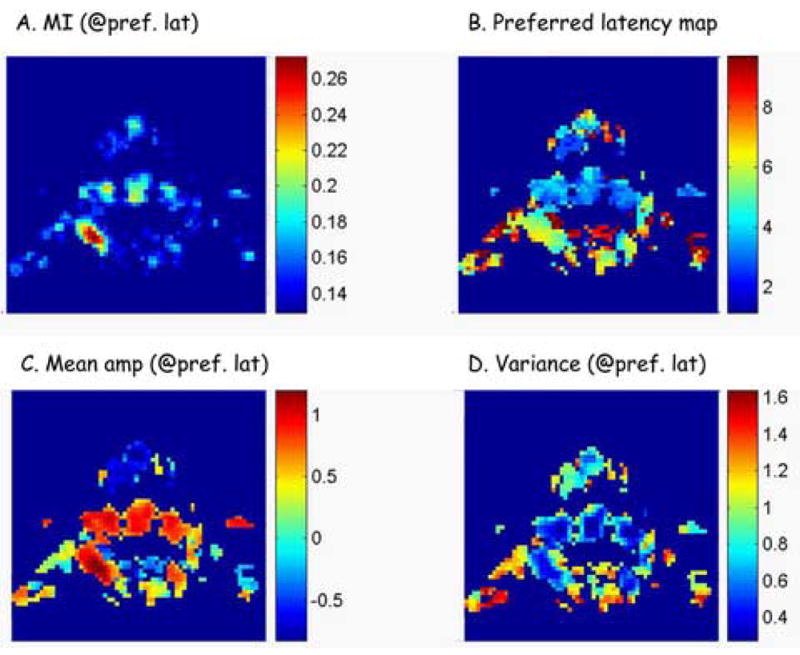
A. Mutual information values for significantly informative (LEARN-related) voxels. MI values are shown for the latencies in which each voxel is most informative about the task. (Axes: Anterior-posterior: top-bottom). B. Preferred latency map (s) for the corresponding voxels as in A (See also Fig. 3). C. Mean amplitude change (after z-norm) of event-related responses at preferred latencies of individual voxels. D. Variance of responses to single events at the preferred latencies relative to the chosen task condition.

Figure 8.

MI, M- and V-latency maps for 9 of the subjects (for all subjects, approximately the same brain slice is shown). Maps are shown in native space. In all maps, latencies are shown for the significantly informative voxels. Top: MI preferred latency. Middle: M-preferred latencies at which the mean event-related response, averaged over all events, is maximal. Bottom: V-preferred latencies at which minimal variability of event-related responses is observed.

Amplitude of response at best coding latency

For each voxel we computed the mean amplitude of all event-related responses at the preferred latency of the voxel. Amplitudes of event-related responses are determined after z-normalization of the voxel’s signal (see also Methods). Amplitude maps show the mean amplitude of event-related response at the preferred latency, averaged over all events. Combining the information of the amplitude maps (Fig. 7C) with latency maps (Fig. 7B) enables one to acquire at glance, a great deal of information regarding functional organization in the whole brain. It is clear for example, that for this subject, brain areas in the motor network (M1, SMA, PM), as well as the PPC, are all increasing their activation when processing the task condition, with the left PPC showing increased activity significantly later than unimodal motor areas, and that the prefrontal activation is of a decreasing nature, with variable latencies, some of which are at significantly later times.

M,V-localization and M,V-Latency maps

Mutual information, computed for each voxel according to changes in the conditional distributions of responses relative to the unconditional distribution of all responses, is dependent on the estimated distribution of responses, which in turn depend on both the mean and variance of responses. Therefore, as a complementary issue, task-related activation was addressed by computing the maximal average changes in the event-related BOLD response separately (M-maps), as well as the minimal variance of responses following the chosen condition (V-maps). For comparison of spatial localization of task-related activity we show in Fig. 5, for each subject, the same number of most task-related voxels, as determined by each of the three approaches.

In addition, preferred M-latencies were determined as the latencies that maximize mean of maximal (peak) event-related response, averaged over all events. Similarly, preferred V-latencies were defined as the latencies in which the variance in the event-related response is minimal. Both M-latency and V-latency maps were constructed (Fig. 8). We found that localization using M-values was far noisier, with much more false activation outside the brain, as compared to localization according to maximal mutual information, as well as according to minimal event-related variance (see Fig. 5). Both MI and V-localizations were better confined to brain regions. However, in terms of temporal analysis, M-latency maps seem more spatially structured, and possibly more consistent across subjects, as compared with the preferred latency maps constructed according to MI and variance analysis (Fig. 8).

Latency of specific ROIs using the different methods

Due to observed similarities in latency maps across subjects (Fig. 8), we attempted to determine a sequence of ROI activations, according to grand average of spatial latency maps of all subjects. To address propagation of task-related signals between specific regions of interest (ROIs), we compute the average latency of an ROI in two different ways (see Methods). In the first, latency of an ROI is first extracted from the latency maps of individual subjects, each according to its own ROI anatomically defined masks; single subjects’ ROI latencies are then averaged. In the second way, latency of ROI is computed directly from the grand average maps, using grand average ROI masks defined as the union of all bilateral individual subjects’ masks in MNI space.

According to grand average ROI masks, we find the following sequence of task-related information coding: preSMA (5.64 +− 0.021 s), SMA (5.8 +− 0.022 s), PM (6.24 +− 0.006 s), M1 (6.44 +− 0.006 s) and finally PPC (6.46 +− 0.004 s). According to information analysis and individual subjects ROI masks, we find the following sequence of task-related information coding: SMA (5.1905 +− 0.232 s), right PM (5.3534 +− 0.292 s), left PM (5.5173 +− 0.292 s), preSMA (5.6472 +− 0.237 s), left PPC (5.6754 +− 0.143 s), left M1 (5.919 +− 0.25 s), right PPC (6.0108 +− 0.322 s), and finally right M1 (6.5508 +− 0.339 s). In both cases, the informative response in SMA is significantly earlier than the informative responses in the both primary motor cortices, as well as the PPC.

Examining the individual subjects’ latency maps (as in Fig. 8), we observe within the PPC (mainly on the left hemisphere), in some slices- a traveling wave of task-related activity, which starts at medial portions of the PPC, and expands gradually into lateral portions of the PPC. This pattern of activation is seen in many of the subjects, both in I-latency maps as well as in M-latency maps. We note that ROI analysis of latency maps is in some cases a simplification of the detailed spatial distribution of latencies, representing the temporal spread of brain activity.

According to the analysis on grand average M-latency maps, using grand average ROI masks, we estimate the following sequence of activation: SMA (4.13 +− 0.01 s), PM (4.61 +− 0.005 s), preSMA (4.53 +− 0.014 s), M1 (4.66 +− 0.006 s), and PPC (5.04 +− 0.005 s).

Comparison of the latencies determined according to the different methods reveal that ROI latencies determined according to mutual information were typically longer than those determined according to M-latency maps, suggesting that the time in which the event-related BOLD response is most informative about the task condition is not at the peak of the response, but rather 1–2 s later.

Finally, the same analysis was performed on V-latency maps. Using grand average ROI masks we find the following estimation of activation sequence: M1 (4.45+− 0.007 s), PM (4.56 +− 0.006 s), SMA (4.64 +− 0.017 s), preSMA (4.67 +− 0.018 s) and PPC (4.86 +− 0.005 s).

Preferred Latency Differences between Pairs of Regions of Interest (ROIs), Regardless of the Stimulus Pattern

The information analysis presented thus far, computes the information between the hemodynamic response and the preceding task condition. Therefore, it requires knowledge of the experimental design. Namely, the information content of a response is tested with respect to a specific design that we assume to affect the responses. However, it is clear that activity of cortical neurons is not associated uniquely with the experimentally studied paradigm, but is also affected by background information processing. It is of interest, therefore, to study mutual information between different regions of interest (ROIs), irrespective of the stimulus pattern. This enables one to study possible interactions during information processing, which are not necessarily related to an imposed experimental paradigm. Moreover, the approach could be used to study of information interactions between ROIs during the processing of any arbitrary stimulus pattern, in particular that of natural stimuli.

Therefore, in this case, rather than computing the mutual information between the event-related responses of an ROI and the experimentally designed task condition, here we compute the mutual information between the mean event-related signals of two different ROIs, each averaged over all voxels within the ROI. The continuous signal from each ROI is taken as a whole, rather than just task-related portions of it, as in the previous analysis. In order to estimate the probability distributions of the responses, the signal in one of the ROIs is considered as the “stimulus” and the distributions of the responses of the second ROI, both unconditioned and conditioned on the signal amplitude in the first ROI, are estimated. The responses of the second ROI are those that follow the signal in the first by a chosen latency dt. We compute this for both positive and negative values of dt, to construct plots as the one presented in Fig. 9 (solid line). We then estimate at which latency signals in the two ROIs are most informative about one another; namely, the latency in which the signal in one ROI is most informative about the signal that preceded, or followed it, in the other ROI. It can be seen that, for instance in the case of this subject, in terms of information content within the signals, SMA preferably precedes left PM by approximately 1s, pre SMA precedes left PPC by 1.5s, left PPC follows right PPC by about 0.5–1s, while SMA and pre SMA are most informative about each other’s activity with zero delay between their signals.

Figure 9.

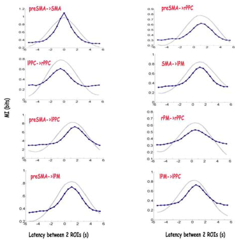
Mutual information between the signals in pairs of ROIs, plotted as a function of the time delay between their activities (solid line). Positive latencies means the “stimulus” ROI precedes the other ROI, whereas negative means the opposite relation. Results are presented for the same subject as in Fig. 3 and Fig. 5. For comparison, results for time delayed correlation analysis between the times series of the two ROIs are presented (dashed line).

For comparison, we also compute the simple linear correlation between the two regions at varying time lags (Fig. 9, dashed lines). In the case of study, where the signals in the different ROIs seem to be noisy time-shifted versions of one another, the results from the correlation analysis are similar to those from the information analysis. In the general case, information analysis would be superior if there is a non linear relation between the amplitudes of response in the time-lagged time series from the two ROIs.

Discussion

A new approach for the analysis of event-related BOLD signals is proposed. The analysis is based on computing the mutual information (MI) between a stimulus function, and the corresponding event-related BOLD response. The approach is useful both for spatial localization of task-related activity, as well as for extracting temporal information about the dynamic propagation of task-related activity in the brain.

In the basic analysis we regard the experimental design as the stimulus function, and compute the MI between a specific task condition (in the example presented in this study- a motor learning condition) and the amplitude of event-related BOLD response that follows it by certain latency (dt). For each voxel, we define a preferred latency as the latency which maximizes its information content about the stimulus (task-condition). We perform a whole brain analysis and choose task-related voxels as those whose signal contains the highest information content about the stimulus condition, each voxel at its own preferred latency.

This approach is an alterative approach to spatial localization of task-related activity that is most commonly performed using the standard GLM analysis. Standard GLM analysis is based on two questionable assumptions. The first is that the hemodynamic response function (HRF) of all voxels in the brain is fixed, an assumption which is known to be inaccurate [Aguirre et al., 1998; Silva and Koretsky, 2002]. In fact, localization is sensitive to the model function in use, and differences in the areas which are highlighted could be observed when different HRFs are used as model functions [Handwerker et al., 2004].

The second assumption is that there exists a linear relation between the stimulus and BOLD response, an assumption which at least in some cases has been shown to be erroneous [Boynton et al., 1996; Friston et al., 1998; Glover, 1999; Huettel and McCarthy, 2000; Liu and Gao, 2000; Kershaw et al., 2001]. One of the advantages of the information theoretic approach is that it is model free. There are no assumptions about the shape and delay of HRF and it can actually account for each voxel having its unique response dynamics. Additionally, no linearity assumptions are required regarding the nature of stimulus-response transformation either.

In this approach, task related activity is associated with areas that show both increased, as well as decreased activation, relative to baseline activity, during task-performance. Since the computed MI for a voxel is insensitive to whether there is an increase or decrease of the signal in response to a task-condition, localization of task-related activity is not restricted to areas which show an increase in the BOLD signal. In fact, by looking at the average event-related magnitude of response of voxels at their preferred latencies, we find that in the case of a motor learning task- some regions which are highly informative about the task condition actually decrease their responses following its presentation. These areas are mostly found in prefrontal regions and posterior lateral cortex. The regions found in this study to be involved in the task by decreased responses, are areas that were previously reported as the default network in the brain. Those regions of the brain are associated with spontaneous activity of cortical networks, and are regularly observed to decrease their activity during attention demanding cognitive tasks [Gusnard and Raichle, 2001; Raichle et al., 2001], as is the case in learning of a motor task presented in this study.

By comparing spatial localization of task-related activation using the suggested information-theoretic approach, with the results obtained using standard GLM analysis, we find the main difference to be in prefrontal regions. According to standard GLM analysis, little task-related activity in prefrontal regions was observed, relative to more extended areas of activation observed using information analysis. However, it is well known that prefrontal regions are involved in motor planning, execution and monitoring [Gehring and Knight, 2000]. Study of event-related responses of voxels in these regions suggests that this difference is mainly due to atypical HRFs of the voxels, as compared to the typical HRFs observed in primary sensori-motor areas for example. Many voxels in these areas exhibit an HRF response, which is relatively shifted in time. The HRF of some other voxels in these regions has a somewhat step-like, non-peaky, shape. By using broader or shifted HRFs- more elaborated task-related activations could be revealed in these regions even in the framework of GLM analysis [Solbakk, 2005]. This again, stresses even further the importance of using non-uniform HRFs for whole brain analysis.

The numerous studies that have been performed using GLM analysis with fixed HRF responses have proven the approach to be a very useful method that is successful in identifying activations related to a wide variety of tasks. However, many of these studies focus on activations in primary sensory and motor areas, mainly of normal control groups, typically young students. Fixed shape HRFs may be indeed a good approximation for the typical response of many brain regions of such normal controls. However, application of this approach to other populations, such as aging and patient populations, has been a constant challenge [D’Esposito et al., 2003]. We expect that localization of task-related activation would be particularly sensitive to the fixed-HRF assumption, at higher association brain regions, and at subject populations, in which untypical HRFs are commonly observed [Pineiro et al., 2002; Rother et al., 2002; Hamzei et al., 2003]. Under theses circumstances, we predict that the information-theoretic method may be superior over the model based GLM analysis. The information-theoretic method may be more sensitive and reveal more task-related activations in higher order association regions and in populations with less typical HRFs, including older controls, and patients with neurological disorders, particularly if they involve vascular pathology.

We demonstrated that the information theoretic approach for the analysis of fMRI data, allows us to localize task-related activity and determine the average amplitudes of responses simultaneously. This method can be used to combine amplitude and spatial localization aspects of information about brain activity together with temporal information, which is also extracted from the data. Therefore, in addition to localizing task-related activity and determining whether it is associated with increased or decreased responses, we also construct spatio-temporal maps of preferred latencies for each voxel. These maps enable whole-brain visualizations of the spread of task-related informative signals within the brain. We found informative activity in the SMA about the task condition, precedes the informative activity in PM, M1 and PPC, with a delay of approximately 650 ms between SMA and M1. These results are in accordance to results obtained by a different approach, based on coherence measures for latency analysis applied to the same data set [Sun et al., 2005].

For comparison, latency maps were also determined in two other ways. M-Latency maps are maps of the latency of the average event-related maximal response. V-latency maps are maps showing the latency of minimal variance in the responses to single events. In all cases, latency of task-related informative activation was shortest for SMA, primary and motor cortices, and longest for the PPC. M-latencies were typically shorter than those computed to maximize information coding, suggesting that the time in which the event-related BOLD response is most informative about the task condition is not at the peak of the response, but rather 1–2 s later.

We also observed subdivisions within our regions of interest, in terms of information flow. In particular, the activity within the left PPC seems to propagate from medial to lateral subregions in the PPC, as is observed in individual subjects’ latency maps, computed according to all three methods.

Due to the gap in our understanding of the relation between the latencies of BOLD responses and the underlying latencies of neuronal activity, it is hard to conclude which latency map represents more reliably the underlying sequence of neuronal activation [Logothetis et al., 2001; Henson et al., 2002; Nevado et al., 2004]. In terms of the underlying neural responses, a delayed event-related response could be the result of a delayed neural response, as well as of an extended neuronal processing time [Henson et al., 2002]. The BOLD response is affected by both, and therefore a sequence of activation determined according to BOLD responses does not map easily to the sequence of activation of neuronal populations. Nevertheless, the fact that there are consistencies in event-related latency maps across subjects suggests that these latencies have a meaningful relation to the task related neuronal activity. Future studies, possibly combining fMRI, EEG, as well intra- or extra-cellular recordings, may help clarify these issues.

In terms of temporal analysis of the BOLD responses, we perform an additional analysis on the data. In this case, we perform the analysis on the mean signals extracted from pairs of specific regions of interest (ROIs), and regard the signal from one ROI as the stimulus to the other ROI. We compute the MI between the amplitudes of the signals in the two ROIs for various possible time delays between the two signals. We find that in most cases there is a peak of MI value around a particular latency between the two signals, suggesting that in terms of information content, the signal in one ROI precedes, or lags after, that of the other ROI with that latency. Here we show, for example, that SMA preferably precedes left PM by approximately 1s, pre SMA precedes left PPC by 1.5s, left PPC follows right PPC by about 0.5–1s, and that the signals of SMA and pre SMA are most informative about each other’s activity with zero delay [Ikeda et al., 1992; Kansaku et al., 1998; Menon et al., 1998; Weilke et al., 2001; Sun et al., 2005].

Information analysis between the two signals, in this case, does not rely on knowledge of the experimentally designed stimulus pattern. Therefore, it is not confined to the study of artificially designed experimental paradigm, and can thus allow the study of functional connectivity during information processing of natural stimuli.

Moreover, this approach to studying the preferred latency of mutual information between two signals is easily elaborated to the study of EEG data and intracranial recordings, both of which provide brain signals that are of higher temporal resolution and better understood in terms of their relation to the underlying neural processes. In these cases, information is computed between the event-related signals recorded from two electrodes, and the preferred latency is determined.

While the information-theoretic approach suggested here for the spatio-temporal analysis of fMRI and EEG data is powerful, there are limitations to the approach. Mutual information analysis requires a large data set, namely, many repetitions of the event (>200, depending on the SNR, as well as specificity of responses to the chosen condition). Moreover, in terms of temporal analysis, we assume that there exists stationarity in the sequence of brain activations within the analyzed time period (i.e. that one ROI is always responsive before the other) and that there is some time point in the event-related response at which information reaches a peak. If the event-related response of a voxel is not characterized by a peaked response, spatial localization of task-related activation is possible, however, the determined preferred latency of the voxel will be mainly affected by noise. Finally, we wish to note that our analysis provides information regarding the sequence of activations of different brain areas; however, these sequences do not imply causal relations between different areas, only the relative times at which their signals are most informative about one another, since they may as well be driven by a common source with variable delays. Assessing causal relations between different brain regions is of extreme importance to our understanding of functional connectivity, and while some attempts have been made to address this issue, mainly using the concept of granger causality [Goebel et al., 2003], more studies in this direction are required.

References

- Aguirre GK, Zarahn E, D’Esposito M. The variability of human, BOLD hemodynamic responses. Neuroimage. 1998;8:360–369. doi: 10.1006/nimg.1998.0369. [DOI] [PubMed] [Google Scholar]
- Arfanakis K, Cordes D, Haughton VM, Moritz CH, Quigley MA, Meyerand ME. Combining independent component analysis and correlation analysis to probe interregional connectivity in fMRI task activation datasets. Magn Reson Imaging. 2000;18:921–930. doi: 10.1016/s0730-725x(00)00190-9. [DOI] [PubMed] [Google Scholar]
- Bellgowan PS, Saad ZS, Bandettini PA. Understanding neural system dynamics through task modulation and measurement of functional MRI amplitude, latency, and width. Proc Natl Acad Sci U S A. 2003;100:1415–1419. doi: 10.1073/pnas.0337747100. [DOI] [PMC free article] [PubMed] [Google Scholar]
- Borst A, Theunissen FE. Information theory and neural coding. Nat Neurosci. 1999;2:947–957. doi: 10.1038/14731. [DOI] [PubMed] [Google Scholar]
- Boynton GM, Engel SA, Glover GH, Heeger DJ. Linear systems analysis of functional magnetic resonance imaging in human V1. J Neurosci. 1996;16:4207–4221. doi: 10.1523/JNEUROSCI.16-13-04207.1996. [DOI] [PMC free article] [PubMed] [Google Scholar]
- Buxton RB. Introduction to Functional Magnetic Resonance Imaging: Principles & Techniques. New York: Cambridge University Press; 2002. [Google Scholar]
- Calhoun V, Adali T, Kraut M, Pearlson G. A weighted least-squares algorithm for estimation and visualization of relative latencies in event-related functional MRI. Magn Reson Med. 2000;44:947–954. doi: 10.1002/1522-2594(200012)44:6<947::aid-mrm17>3.0.co;2-5. [DOI] [PubMed] [Google Scholar]
- Cover TM, Thomas JA. Elements of information theory. New York: Wiley; 1991. [Google Scholar]
- Dale AM, Buckner RL. Selective averaging of rapidly presented individual trials using fMRI. Human Brain Mapping. 1997;5:329–340. doi: 10.1002/(SICI)1097-0193(1997)5:5<329::AID-HBM1>3.0.CO;2-5. [DOI] [PubMed] [Google Scholar]
- de Araujo DB, Tedeschi W, Santos AC, Elias J, Jr, Neves UP, Baffa O. Shannon entropy applied to the analysis of event-related fMRI time series. Neuroimage. 2003;20:311–317. doi: 10.1016/s1053-8119(03)00306-9. [DOI] [PubMed] [Google Scholar]
- de Ruyter van Steveninck RR, Lewen GD, Strong SP, Koberle R, Bialek W. Reproducibility and variability in neural spike trains. Science. 1997;275:1805–1808. doi: 10.1126/science.275.5307.1805. [DOI] [PubMed] [Google Scholar]
- D’Esposito M, Deouell LY, Gazzaley A. Alterations in the BOLD fMRI signal with ageing and disease: a challenge for neuroimaging. Nat Rev Neurosci. 2003;4:863–872. doi: 10.1038/nrn1246. [DOI] [PubMed] [Google Scholar]
- Duvernoy HM. The Human Brain: Surface, Blood Supply, and Three Dimensional Sectional Anatomy. 2. Springer; Vienna: 1999. [Google Scholar]
- Formisano E, Goebel R. Tracking cognitive processes with functional MRI mental chronometry. Curr Opin Neurobiol. 2003;13:174–181. doi: 10.1016/s0959-4388(03)00044-8. [DOI] [PubMed] [Google Scholar]
- Formisano E, Linden DE, Di Salle F, Trojano L, Esposito F, Sack AT, Grossi D, Zanella FE, Goebel R. Tracking the mind’s image in the brain I: time-resolved fMRI during visuospatial mental imagery. Neuron. 2002;35:185–194. doi: 10.1016/s0896-6273(02)00747-x. [DOI] [PubMed] [Google Scholar]
- Friston KJ, Josephs O, Rees G, Turner R. Nonlinear event-related responses in fMRI. Magn Reson Med. 1998;39:41–52. doi: 10.1002/mrm.1910390109. [DOI] [PubMed] [Google Scholar]
- Friston KJ, Holmes AP, Worsley KJ, Poline JP, Frith CD, Frackowiak RSJ. Statistical Parametric Maps in Functional Imaging: A General Linear Approach. Human Brain Mapping. 1995;2:189–210. [Google Scholar]
- Fuhrmann G, Segev I, Markram H, Tsodyks M. Coding of temporal information by activity-dependent synapses. J Neurophysiol. 2002;87:140–148. doi: 10.1152/jn.00258.2001. [DOI] [PubMed] [Google Scholar]
- Gehring WJ, Knight RT. Prefrontal-cingulate interactions in action monitoring. Nat Neurosci. 2000;3:516–520. doi: 10.1038/74899. [DOI] [PubMed] [Google Scholar]
- Glover GH. Deconvolution of impulse response in event-related BOLD fMRI. Neuroimage. 1999;9:416–429. doi: 10.1006/nimg.1998.0419. [DOI] [PubMed] [Google Scholar]
- Goebel R, Roebroeck A, Kim DS, Formisano E. Investigating directed cortical interactions in time-resolved fMRI data using vector autoregressive modeling and Granger causality mapping. Magn Reson Imaging. 2003;21:1251–1261. doi: 10.1016/j.mri.2003.08.026. [DOI] [PubMed] [Google Scholar]
- Goldman MS, Maldonado P, Abbott LF. Redundancy reduction and sustained firing with stochastic depressing synapses. J Neurosci. 2002;22:584–591. doi: 10.1523/JNEUROSCI.22-02-00584.2002. [DOI] [PMC free article] [PubMed] [Google Scholar]
- Gusnard DA, Raichle ME. Searching for a baseline: functional imaging and the resting human brain. Nat Rev Neurosci. 2001;2:685–694. doi: 10.1038/35094500. [DOI] [PubMed] [Google Scholar]
- Hamzei F, Knab R, Weiller C, Rother J. The influence of extra- and intracranial artery disease on the BOLD signal in FMRI. Neuroimage. 2003;20:1393–1399. doi: 10.1016/S1053-8119(03)00384-7. [DOI] [PubMed] [Google Scholar]
- Handwerker DA, Ollinger JM, D’Esposito M. Variation of BOLD hemodynamic responses across subjects and brain regions and their effects on statistical analyses. Neuroimage. 2004;21:1639–1651. doi: 10.1016/j.neuroimage.2003.11.029. [DOI] [PubMed] [Google Scholar]
- Henson RN, Price CJ, Rugg MD, Turner R, Friston KJ. Detecting latency differences in event-related BOLD responses: application to words versus nonwords and initial versus repeated face presentations. Neuroimage. 2002;15:83–97. doi: 10.1006/nimg.2001.0940. [DOI] [PubMed] [Google Scholar]
- Hernandez L, Badre D, Noll D, Jonides J. Temporal sensitivity of event-related fMRI. Neuroimage. 2002;17:1018–1026. [PubMed] [Google Scholar]
- Huettel SA, McCarthy G. Evidence for a refractory period in the hemodynamic response to visual stimuli as measured by MRI. Neuroimage. 2000;11:547–553. doi: 10.1006/nimg.2000.0553. [DOI] [PubMed] [Google Scholar]
- Ikeda A, Luders HO, Burgess RC, Shibasaki H. Movement-related potentials recorded from supplementary motor area and primary motor area. Role of supplementary motor area in voluntary movements. Brain. 1992;115 ( Pt 4):1017–1043. doi: 10.1093/brain/115.4.1017. [DOI] [PubMed] [Google Scholar]
- Josephs O, Turner R, Friston K. Event-related fMRI. Human Brain Mapping. 1997;5:243–248. doi: 10.1002/(SICI)1097-0193(1997)5:4<243::AID-HBM7>3.0.CO;2-3. [DOI] [PubMed] [Google Scholar]
- Kang K, Shapley RM, Sompolinsky H. Information tuning of populations of neurons in primary visual cortex. J Neurosci. 2004;24:3726–3735. doi: 10.1523/JNEUROSCI.4272-03.2004. [DOI] [PMC free article] [PubMed] [Google Scholar]
- Kansaku K, Kitazawa S, Kawano K. Sequential hemodynamic activation of motor areas and the draining veins during finger movements revealed by cross-correlation between signals from fMRI. Neuroreport. 1998;9:1969–1974. doi: 10.1097/00001756-199806220-00010. [DOI] [PubMed] [Google Scholar]
- Kershaw J, Kashikura K, Zhang X, Abe S, Kanno I. Bayesian technique for investigating linearity in event-related BOLD fMRI. Magn Reson Med. 2001;45:1081–1094. doi: 10.1002/mrm.1143. [DOI] [PubMed] [Google Scholar]
- Liao CH, Worsley KJ, Poline JB, Aston JA, Duncan GH, Evans AC. Estimating the delay of the fMRI response. Neuroimage. 2002;16:593–606. doi: 10.1006/nimg.2002.1096. [DOI] [PubMed] [Google Scholar]
- Liu H, Gao J. An investigation of the impulse functions for the nonlinear BOLD response in functional MRI. Magn Reson Imaging. 2000;18:931–938. doi: 10.1016/s0730-725x(00)00214-9. [DOI] [PubMed] [Google Scholar]
- Logothetis NK, Pauls J, Augath M, Trinath T, Oeltermann A. Neurophysiological investigation of the basis of the fMRI signal. Nature. 2001;412:150–157. doi: 10.1038/35084005. [DOI] [PubMed] [Google Scholar]
- McKeown MJ, Makeig S, Brown GG, Jung TP, Kindermann SS, Bell AJ, Sejnowski TJ. Analysis of fMRI data by blind separation into independent spatial components. Hum Brain Mapp. 1998;6:160–188. doi: 10.1002/(SICI)1097-0193(1998)6:3<160::AID-HBM5>3.0.CO;2-1. [DOI] [PMC free article] [PubMed] [Google Scholar]
- Menon RS, Kim SG. Spatial and temporal limits in cognitive neuroimaging with fMRI. Trends Cogn Sci. 1999;3:207–216. doi: 10.1016/s1364-6613(99)01329-7. [DOI] [PubMed] [Google Scholar]
- Menon RS, Luknowsky DC, Gati JS. Mental chronometry using latency-resolved functional MRI. Proc Natl Acad Sci U S A. 1998;95:10902–10907. doi: 10.1073/pnas.95.18.10902. [DOI] [PMC free article] [PubMed] [Google Scholar]
- Miezin FM, Maccotta L, Ollinger JM, Petersen SE, Buckner RL. Characterizing the hemodynamic response: effects of presentation rate, sampling procedure, and the possibility of ordering brain activity based on relative timing. Neuroimage. 2000;11:735–759. doi: 10.1006/nimg.2000.0568. [DOI] [PubMed] [Google Scholar]
- Mohamed MA, Yousem DM, Tekes A, Browner NM, Calhoun VD. Timing of cortical activation: a latency-resolved event-related functional MR imaging study. AJNR Am J Neuroradiol. 2003;24:1967–1974. [PMC free article] [PubMed] [Google Scholar]
- Moritz CH, Haughton VM, Cordes D, Quigley M, Meyerand ME. Whole-brain functional MR imaging activation from a finger-tapping task examined with independent component analysis. AJNR Am J Neuroradiol. 2000;21:1629–1635. [PMC free article] [PubMed] [Google Scholar]
- Nevado A, Young MP, Panzeri S. Functional imaging and neural information coding. Neuroimage. 2004;21:1083–1095. doi: 10.1016/j.neuroimage.2003.10.043. [DOI] [PubMed] [Google Scholar]
- Noll DCSVA, Vazquez AL, Peltier SJ. Spiral Scanning in fMRI. In: Moonen CTWBP, editor. Functional MRI. New York: Springer; 2000. pp. 149–160. [Google Scholar]
- Panzeri S, Pola G, Petersen RS. Coding of sensory signals by neuronal populations: the role of correlated activity. Neuroscientist. 2003;9:175–180. doi: 10.1177/1073858403009003010. [DOI] [PubMed] [Google Scholar]
- Paz R, Boraud T, Natan C, Bergman H, Vaadia E. Preparatory activity in motor cortex reflects learning of local visuomotor skills. Nat Neurosci. 2003;6:882–890. doi: 10.1038/nn1097. [DOI] [PubMed] [Google Scholar]
- Picard N, Strick PL. Imaging the premotor areas. Curr Opin Neurobiol. 2001;11:663–672. doi: 10.1016/s0959-4388(01)00266-5. [DOI] [PubMed] [Google Scholar]
- Pineiro R, Pendlebury S, Johansen-Berg H, Matthews PM. Altered hemodynamic responses in patients after subcortical stroke measured by functional MRI. Stroke. 2002;33:103–109. doi: 10.1161/hs0102.100482. [DOI] [PubMed] [Google Scholar]
- Raichle ME, MacLeod AM, Snyder AZ, Powers WJ, Gusnard DA, Shulman GL. A default mode of brain function. Proc Natl Acad Sci U S A. 2001;98:676–682. doi: 10.1073/pnas.98.2.676. [DOI] [PMC free article] [PubMed] [Google Scholar]
- Reich DS, Mechler F, Victor JD. Independent and redundant information in nearby cortical neurons. Science. 2001;294:2566–2568. doi: 10.1126/science.1065839. [DOI] [PubMed] [Google Scholar]
- Richter W, Somorjai R, Summers R, Jarmasz M, Menon RS, Gati JS, Georgopoulos AP, Tegeler C, Ugurbil K, Kim SG. Motor area activity during mental rotation studied by time-resolved single-trial fMRI. J Cogn Neurosci. 2000;12:310–320. doi: 10.1162/089892900562129. [DOI] [PubMed] [Google Scholar]
- Rother J, Knab R, Hamzei F, Fiehler J, Reichenbach JR, Buchel C, Weiller C. Negative dip in BOLD fMRI is caused by blood flow--oxygen consumption uncoupling in humans. Neuroimage. 2002;15:98–102. doi: 10.1006/nimg.2001.0965. [DOI] [PubMed] [Google Scholar]
- Saad ZS, DeYoe EA, Ropella KM. Estimation of FMRI response delays. Neuroimage. 2003;18:494–504. doi: 10.1016/s1053-8119(02)00024-1. [DOI] [PubMed] [Google Scholar]
- Schneidman E, Bialek W, Berry MJ., 2nd Synergy, redundancy, and independence in population codes. J Neurosci. 2003;23:11539–11553. doi: 10.1523/JNEUROSCI.23-37-11539.2003. [DOI] [PMC free article] [PubMed] [Google Scholar]
- Silva AC, Koretsky AP. Laminar specificity of functional MRI onset times during somatosensory stimulation in rat. Proc Natl Acad Sci U S A. 2002;99:15182–15187. doi: 10.1073/pnas.222561899. [DOI] [PMC free article] [PubMed] [Google Scholar]
- Simon O, Mangin JF, Cohen L, Le Bihan D, Dehaene S. Topographical layout of hand, eye, calculation, and language-related areas in the human parietal lobe. Neuron. 2002;33:475–487. doi: 10.1016/s0896-6273(02)00575-5. [DOI] [PubMed] [Google Scholar]
- Simoncelli EP, Olshausen BA. Natural image statistics and neural representation. Annu Rev Neurosci. 2001;24:1193–1216. doi: 10.1146/annurev.neuro.24.1.1193. [DOI] [PubMed] [Google Scholar]
- Solbakk AK, Hale L, Fuhrmann Alpert G, Furst A, Oga T, Suppiah S, Pickard N, Knight RT. Reduced anterior cingulate gyrus activation in normal aging: An event-related fMRI study; CNS 2005 Annual Meeting; New York, NY. 2005. [Google Scholar]
- Sun FT, Miller LM, D’Esposito M. Measuring temporal dynamics of functional networks using phase spectrum of fMRI data. Neuroimage. 2005;28:227–237. doi: 10.1016/j.neuroimage.2005.05.043. [DOI] [PubMed] [Google Scholar]
- Swinnen SP. Intermanual coordination: from behavioural principles to neural-network interactions. Nat Rev Neurosci. 2002;3:348–359. doi: 10.1038/nrn807. [DOI] [PubMed] [Google Scholar]
- Vazquez AL, Noll DC. Nonlinear aspects of the BOLD response in functional MRI. Neuroimage. 1998;7:108–118. doi: 10.1006/nimg.1997.0316. [DOI] [PubMed] [Google Scholar]
- Victor JD. How the brain uses time to represent and process visual information(1) Brain Res. 2000;886:33–46. doi: 10.1016/s0006-8993(00)02751-7. [DOI] [PubMed] [Google Scholar]
- Visscher KM, Miezin FM, Kelly JE, Buckner RL, Donaldson DI, McAvoy MP, Bhalodia VM, Petersen SE. Mixed blocked/event-related designs separate transient and sustained activity in fMRI. Neuroimage. 2003;19:1694–1708. doi: 10.1016/s1053-8119(03)00178-2. [DOI] [PubMed] [Google Scholar]
- Weilke F, Spiegel S, Boecker H, von Einsiedel HG, Conrad B, Schwaiger M, Erhard P. Time-resolved fMRI of activation patterns in M1 and SMA during complex voluntary movement. J Neurophysiol. 2001;85:1858–1863. doi: 10.1152/jn.2001.85.5.1858. [DOI] [PubMed] [Google Scholar]
- Willingham DB. A neuropsychological theory of motor skill learning. Psychol Rev. 1998;105:558–584. doi: 10.1037/0033-295x.105.3.558. [DOI] [PubMed] [Google Scholar]
- Worsley KJ, Friston KJ. Analysis of fMRI time-series revisited--again. Neuroimage. 1995;2:173–181. doi: 10.1006/nimg.1995.1023. [DOI] [PubMed] [Google Scholar]
- Yousry TA, Schmid UD, Alkadhi H, Schmidt D, Peraud A, Buettner A, Winkler P. Localization of the motor hand area to a knob on the precentral gyrus. A new landmark. Brain. 1997;120 ( Pt 1):141–157. doi: 10.1093/brain/120.1.141. [DOI] [PubMed] [Google Scholar]
Associated Data
This section collects any data citations, data availability statements, or supplementary materials included in this article.