Knowledge discovery processing and data mining in karyometry

Abstract

Objective

This article presents the rationale for applying different sequences of multivariate analysis algorithms to determine if and where, in the large and high dimensional data space, events have led to change in karyometric features. Such procedures have become known as knowledge discovery processing, or data mining. The objective is to reveal the structure of the data under analysis, and the algorithms are used as tools to this end. A statistical significance statement is attained to secure the biologic interpretation.

Materials

Clinical materials and results from the analysis of four studies were used: the demonstration of chemopreventive efficacy of letrozole in a situation where only a small subset of cells is affected; the detection of a pre-neoplastic lesion in colorectal tissue; data processing to document clues that predict risk of recurrence of a bladder lesion; and the use of metafeatures and second order discriminant analysis in a study of efficacy of Vitamin A in the chemoprevention of skin lesions.

Results

Evidence for chemopreventive efficacy was demonstrated in the first example only after processing identified the small subpopulation of affected nuclei in a study of breast epithelial cells. Detection of a pre-neoplastic development is linked to a progression curve connecting nuclei from normal tissue to nuclei from pre-malignant colorectal lesions. The prediction of risk of recurrence of papillary bladder lesions is possible by detecting changes in nuclei of a certain phenotype. Efficacy of Vitamin A as a chemopreventive agent for skin cancer could be demonstrated with a dose response curve after a second order discriminant analysis was employed.

Conclusions

The information of biologic interest would, in none of these instances, have been revealed by a straightforward single algorithmic analysis.

Introduction

Karyometry has brought objective measurement to the assessment of histopathologic samples. It has also resulted in the ability to detect, and statistically secure, very small differences in the spatial and statistical distribution of nuclear chromatin, differences too subtle to be detected by visual observation [1, 2]. A number of applications take advantage of the increased sensitivity of detection. There has been the discovery of pre-neoplastic lesions in histologically “normal-appearing” tissue [3, 4]. There has been the detection of multiple, statistically distinguishable phenotypes of nuclei in premalignant and malignant lesions [2, 5, 6]. The enhanced sensitivity has allowed measurement of efficacy of chemopreventive intervention. This may have found expression as a small change in the majority of nuclei of the target tissue [7], or in only a minor subset, which after intervention show a reduction in their deviation from normal [8]. There has been the detection of clues to the risk of lesion development, progression or recurrence [9].

The nuclear chromatin pattern reflects the differentiation and functional state of a cell. It may serve as an integrating biomarker that is not limited in its ability to indicate change by particular pathways [10]. The nuclear chromatin offers a rich assortment of diagnostic clues expressed by variables characterizing its spatial and statistical distribution. Most computer packages developed for karyometry [11] offer a rather large number of variables (from 30 to 400), or features, for a mensuration of the nuclear chromatin distribution [12-15].

The events that lead to a change in nuclear differentiation and of the nuclear chromatin pattern find expression in a feature space of high dimensionality. One may see data analysis in karyometry as a search in this high dimensional space for the location of change in variable values, for the nature of such changes (i.e. for the features that are involved) of the magnitude of change, of the trend, and for their statistical significance. In many instances, it may not even be known a priori whether any change in the nuclear chromatin pattern has occurred. This is a task closely related to problems where massive amounts of recorded data have to be searched through for events of interest. Such problems are commonly addressed by data mining [16], or knowledge discovery processing [17].

Many of the analytical procedures used in karyometry have their basis in multivariate statistical algorithms. Here, these are not used primarily to establish some statistical significance. Rather, they are applied as tools in data mining to reveal the structure of the data. It is the structure of the data sets that allows an interpretation. Only then is an evaluation of the statistical significance of interest.

One typically is dealing with the need to detect a potentially very small change in the presence of often highly variable background information. The target population of nuclei is frequently heterogeneous, and may consist of a number of phenotypes. It should be clear that application of a single algorithm – such as only a straightforward discriminant analysis or a neural net classifier – may not lead to the desired clarification and understanding of the data structure.

It is the objective of this study to describe the sequence of procedures in which a number of the above mentioned applications may reveal sufficient data structure to allow a biologic interpretation.

Materials and Methods

The data used in thus study have all been presented in earlier communications, proper citations of which are provided.

The overall objective of this study is to describe the rationale of applying certain procedures in a particular sequence, the clues that intermediate results provide for the selection of the next procedural step, and which particular information is sought and obtained from each procedure.

Key to the ability to home in on the location in feature space where relevant change occurs, and to sort out which subset of nuclei, if any, are affected, and to following through certain trends of change, is software with specific capabilities for forming and manipulating subsets of data. This very extensive software collection has been developed over the past 30 years at the University of Arizona Optical Science Center in Tucson, originally for the TICAS software used first in research efforts at the University of Chicago [11, 12, 18].

Results

Case study 1: Efficacy of chemopreventive intervention

Chemopreventive intervention can be expected to be most effective in situations where there is a high risk for development of progressive disease, such as in pre-neoplastic or pre-malignant lesions. In either case, changes due to intervention must be expected to be subtle. The material for this exploratory study involved women at high risk for the development of breast cancer [8]. Participants received the aromatase inhibitor, letrozole, for a period of six months. Fine needle aspirate cytologic preparations were collected at baseline and at the end of study.

The processing sequence started with a search for features that had changed from the baseline samples to the end of study samples. The second processing step was a search for features with significant differences between the baseline and end-of-study data sets. The rationale was that nuclei with extreme values for those features were likely to represent the subpopulation with deviations from normal. This search was done by running a Kruskal Wallis test [19]. This test is non-parametric; therefore, it makes no assumptions concerning distribution characteristics of the features. The test is liberal and is able to identify a number of features with significant differences, but this does not necessarily predict high discrimination potential. The test is instead used as a pre-selection tool. The Kruskal Wallis test results, for every feature, in the value of a test statistic and in a p-value for the significance of the value difference found between baseline and end-of-study nuclei. Since about 100 features were tested, a p-level of p < 0.05 implies that there is a one in 20 chance for a spuriously discriminating feature to be declared as significant. In this study, a p-value of p < 0.005 was used to reduce the chance for inclusion of a spuriously significant feature to below one in two hundred.

To enrich those nuclei in the set to be analyzed for an intervention effect, two subpopulations were formed of the 10% nuclei most deviating from normal in the baseline and end-of-study data sets. The 10% figure is arbitrary. It was chosen to retain enough nuclei, without including too many nuclei which are still quite normal. This should result in a more specific feature selection to discriminate between nuclei deviant from normal at baseline, and nuclei after the intervention at end of study.

The processing sequence started with a search for features that had changed from the baseline samples to the end of study samples. It resulted in a list of mean values for features for the baseline and end-of-study samples. The results were not encouraging--the differences were on the order of only a few percent, and expressed in only a modest number of features. The conclusion was that there was either no effect of the agent measurable by karyometry, or, that in these participants, who after all merely were at high risk, only a small proportion of cells showed deviations from normal. Only those few cells could possibly show a response. However, the deviation of feature values was almost completely averaged out by the presence of a great majority of still normal cells.

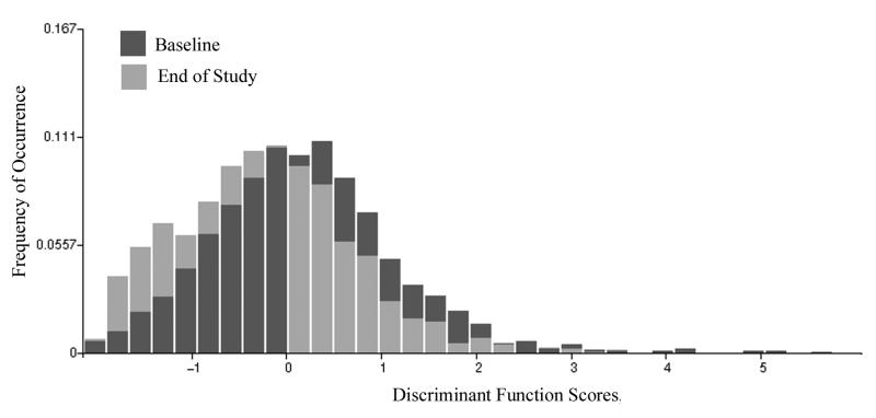
The second processing step was a search for features with significant differences between the baseline and end-of-study data sets. Six of these features were submitted to a stepwise linear discriminant algorithm. The discriminant function DF I,1 resulted in a poor classification success; a correct identification of nuclei as baseline or end-of-study of less than 60% may, in fact, occur by chance. Fig. 1 shows the distributions and the overlap. The discriminant function score distributions show a shift. Two conclusions are drawn. The most prominent features in the discriminant function were those that usually increase in value with increasing deviation from normal. Here, these features undergo a decrease in value; the end-of-study distribution of discriminant function scores is shifted towards lower values, to the left in the plot.

Figure 1.

Distribution of discriminant function scores ( DF I,1 ) for nuclei aspirated at baseline and at the end of study. The distribution undergoes a shift towards negative function values at the end of study, indicating less deviation from normal.

One may assume that nuclei at the higher score value side of the distribution are most deviant from normal. Fig. 1 suggests that there are more such nuclei in the baseline sample than in the end-of-study sample. For the new two subpopulations in the enriched set (10% most deviating from normal), a search for discriminating features was made.

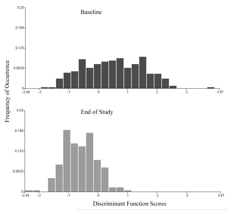
The selected features were submitted to a stepwise linear discriminant algorithm, and a function DF I,2 was derived. The expectation was that for both, the 10% subpopulations of the baseline and the end-of-study samples, the score distributions would be bimodal, but that the mode of nuclei with higher deviations from normal would be diminished in the ES sample. Nuclei with higher deviation from normal have scores in the positive range, to the right in the plot. The score distributions are shown in Fig. 2.

Figure 2.

Distribution of discriminant function scores (DF I,2) for nuclei representing 10% of the nuclei deviating most from normal.

The distribution of scores at baseline shows a broad spread. At the end of study, a distinct shift to less deviation from normal, to the left in the plot, and to negative score values, is observed. The number of nuclei classified as baseline (i.e., expressing deviation from normal) is reduced by a factor of almost four. Estimates are prepared of the number of nuclei deviating from normal at baseline and end of study, and then related to the total number of nuclei recorded. The result is that only about 10% of all nuclei showed deviations from normal in the study participants, and that this percentage was reduced at end of study to about 4%. This reduction, attributed to the intervention, is statistically significant according to the Fleiss Tables.[20] The conclusion is that the agent shows efficacy.

Case study 2: Documenting a pre-neoplastic lesion

The material used in case study 2 were part of a karyometric study of colorectal tissue [21]. The first step in the processing sequence was to establish end points, based on nuclei from normal cases at one extreme, and nuclei from a progressed lesion (e.g. high grade intraepithelial neoplasia) at the other. It is important that the “normal” control nuclei come from patients free of any premalignant or malignant lesion. The end points serve to establish a location and a direction in feature space where the earliest stage of progression, from normal to a pre-neoplastic lesion might be expected. It also provides a first stab at a choice of features.

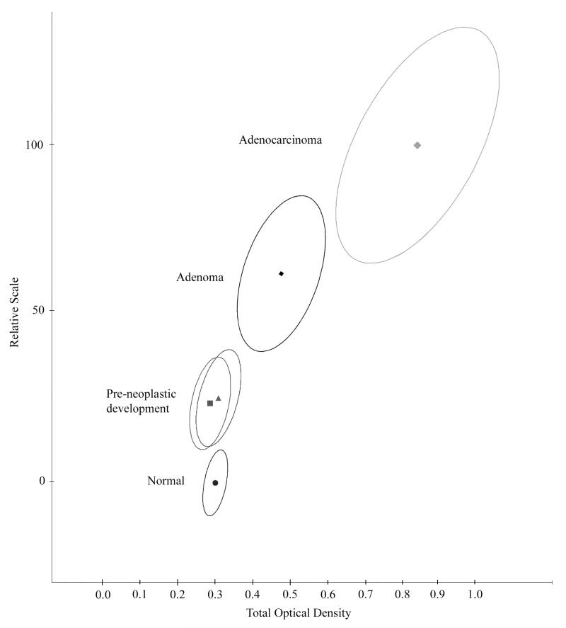
A feature selection procedure was applied, and a discriminant function derived. This function was next applied to every premalignant and early malignant diagnostic category for the organ site (e.g. low grade intraepithelial neoplasia, high grade neoplasia and carcinoma in situ). This allows plotting a progression curve [22] using the discriminant function scores as one variable in a two-dimensional plot, and a suitable other variable, such as total optical density, nuclear area, or average nuclear abnormality, as the second variable. The progression curve is drawn connecting the mean scores for the diagnostic categories. It is instructive to plot the 95% confidence ellipses for nuclei in each of the diagnostic categories to convey an idea of the separation of these diagnostic categories in feature space. The mean discriminant function score, and the confidence ellipse for the nuclei recorded in the histologically normal appearing tissue of the organ harboring a malignant or premalignant lesion are expected to appear along the progression curve between the normal reference nuclei and the lowest grade premalignant lesion.

The progression curve, shown in Fig 3., extends from normal rectal mucosa (norm/norm) to adenoma and to adenocarcinoma. The nuclei recorded in histologically normal-appearing tissue from subjects with colonic lesions (norm/lesion) appear on the progression curve between normal mucosa and adenoma. There appeared to be no difference between nuclei from a pre-neoplastic lesion in case of adenoma, or of adenocarcinoma. The confidence ellipse for the tentative pre-neoplastic lesion is displaced in the expected direction from the normal reference, but it also overlaps the norm/norm data set. Nuclei sampled in such histologically normal-appearing tissue may comprize a substantial number of normal appearing and normal nuclei. This diminishes the separation of the nuclei characterizing the pre-neoplastic development from normal.

Figure 3.

Progression in colonic lesions plotted on a relative scale from zero (mean of zero for nuclei from normal tissue) to 100 (mean for nuclei from adenocarcinoma). Shown are the bivariate mean vectors, and the 95% confidence ellipses for nuclei. The nuclei sampled in histologically normal-appearing tissue from cases harboring an adenoma or an adenocarcinoma lesion (norm/lesion) fall into the same region along the progression curve, between the nuclei from normal tissue ( norm/norm) and from adenoma.

As a next step therefore the norm/lesion data set is submitted to a non-supervised learning algorithm. This will establish whether two statistically different groups of nuclei exist--one matching the norm/norm nuclei, the other more displaced in direction of the lowest pre-malignant lesion, representing a purified set of the pre-neoplastic lesion nuclei. As a feature set for the non-supervised learning procedure one may use the same features as in the initially derived discriminant function. However, a more specific selection might be obtained from a feature selection based on the norm/norm versus the low grade pre-malignant data set.

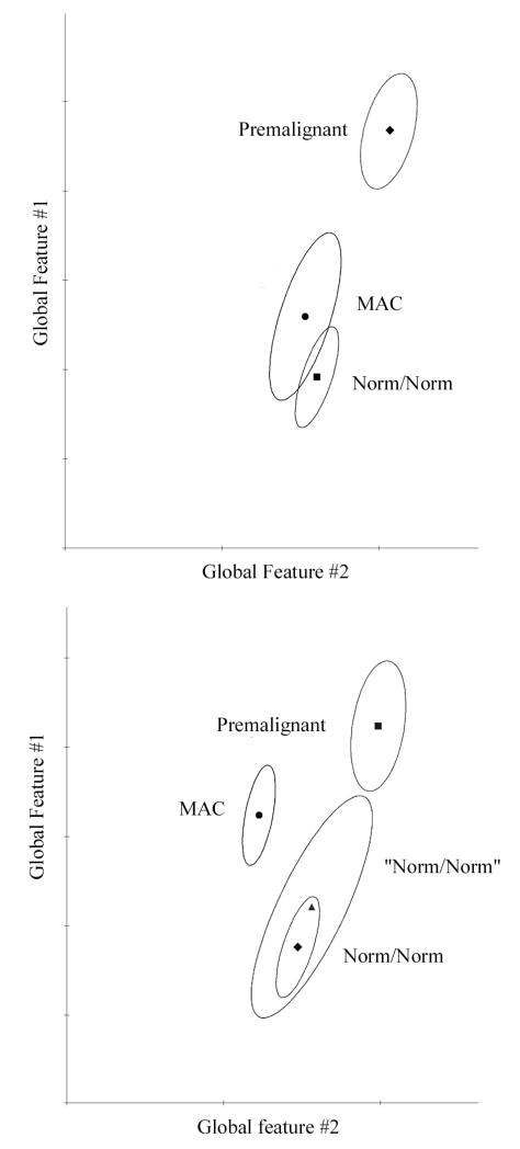
Fig. 4 shows an example for the processing step and the result. The norm/lesion group of nuclei divides into two subgroups. One merges with the norm/norm data set, the other is displaced in direction of the premalignant lesion, and constitutes the purified set of nuclei from the pre-neoplastic lesion.

Figure 4.

Example of heterogeneity in a population of nuclei from a pre-neoplastic lesion. The top figure shows the nuclei from the pre-neoplastic lesion separated from the nuclei from normal tissue. Processing by the non-supervised learning algorithm P-index separates out nuclei truly representing the pre-neoplastic progression, and shows that the remainder nuclei sampled at that location are undistinguishable from normal nuclei (norm/norm).

A non-supervised learning algorithm [23] will always form the number of subgroups – often referred to as “clusters” – that the user specifies. Whether these are to be accepted as statistically significant, different, and valid is decided by a test statistic. Test statistics used in cluster analysis are sometimes based on a reduction of a sum of squares of a distance metric, as it is done in the Beale statistic [24]. That is a very conservative measure. One may find that two clusters, declared not significantly different on the basis of the p-value due to such a test statistic, have widely separated confidence ellipses when a test based on multivariate Gaussian assumptions is applied.

The separation of norm/norm nuclei from norm/lesion nuclei, which establishes the existence of a pre-neoplastic lesion, based on the 95% confidence ellipses for the nuclei, is scientifically interesting, but clinically of little diagnostic value. Clinically, the tolerance ellipses for the case mean values are of interest (e.g. the regions into which a certain percentage of cases, say 90%, are expected to fall with the mean values of their nuclei).

Finally, once the separateness of nuclei from the pre-neoplastic lesion is established, a better distinction from normal may be attained by an additional processing step. Feature selection for non-supervised learning is always an educated guess. But as a result, one has two data sets: norm/norm and norm/lesion. They could be submitted for feature selection and a repeat of the non-supervised learning based on a well-targeted feature set for optimum distinction. The scheme is shown in Table I.

Table I.

Processing scheme alternating supervised and non-supervised learning

1. Establish training sets

2. Feature selection

3. Supervised learning

4. Classification rule

a. Plot of score distributions

5. Processing to check for heterogeneity

a. choice of features for non-supervised learning (educated      guess)

b. non-supervised learning algorithm

c. statistical significance test for subpopulations

6. Processing of subpopulations

a. plot of confidence ellipses for nuclei

b. plot of tolerance ellipses for case means

7. Alternative choice :

a. submit subpopulations to formal feature selection e.g.      Kruskal Wallis test or Genchi & Mori ambiguity measure      [18, 32]

8. Non-supervised learning algorithm with targeted features

9. Statistical significance testing of subpopulations

a. Plot of confidence ellipses for nuclei

b. Plot of tolerance ellipses for case means

10. Supervised learning (e.g. discriminant analysis of subpopulations)

11. Classification rules

a. Plot of score distributions

Case study 3: Risk of lesion recurrence

The identification of cases which pose a high risk for lesion recurrence may involve a lengthy processing sequence. As an example, the processing sequence followed in a study of cases of papillary bladder cancer is presented. The clinical materials in this study consisted of 40 cases who had no recurrence for at least 8 years (NR data set), and 40 cases which had a recurrence (R data set) [9]. The goal of this study was the identification of diagnostic clues that would allow an assessment of risk for recurrence from tissue taken at the time of initial diagnosis. The expectation was that differences in karyometric characteristics, if any, would be small.

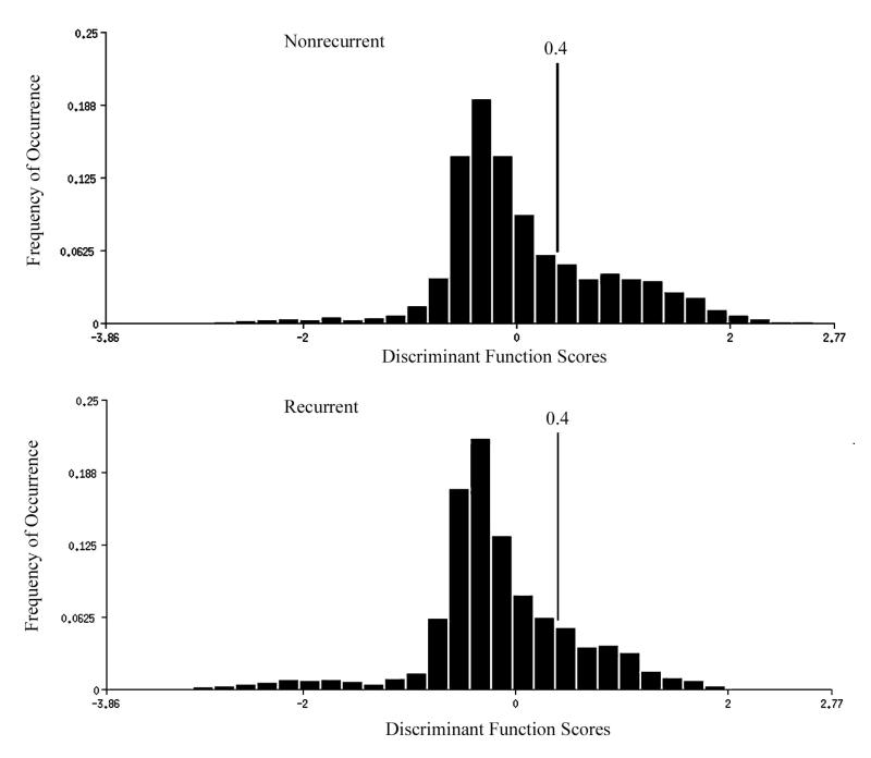
As a first exploratory step in the processing sequence, a Kruskal Wallis test was conducted to identify features with statistically significant differences between the R and NR data sets. An adequate number of such features with p-values < 0.005 was found. A stepwise discriminant analysis (DF I,1) resulted in a score distribution for the R data set with a modest shift towards greater deviation from normal, as seen in Fig. 5. The discriminant algorithm here had assigned the scores with greater deviation from normal to the negative score scale. The relative frequencies of scores in the score range from −1 to – 3 are increased for the cases with recurrence, and the frequencies of scores in the score range +0.4 to +2.0 is decreased in the R data set. The score distributions for both data sets indicated a notable heterogeneity of the nuclear populations.

Figure 5.

Distributions of discriminant function scores DF I,1 for nuclei from cases of papillary bladder cancer of low malignant potential which had a recurrence, and those which had not. The nuclei from recurrent cases show a slight shift in the score distribution. In this instance, the algorithm assigned negative scores to greater deviation from normal. Shown is the threshold set that allowed about 30% of the non-recurrent cases to be recognized in a first stage of a hierarchic classification scheme.

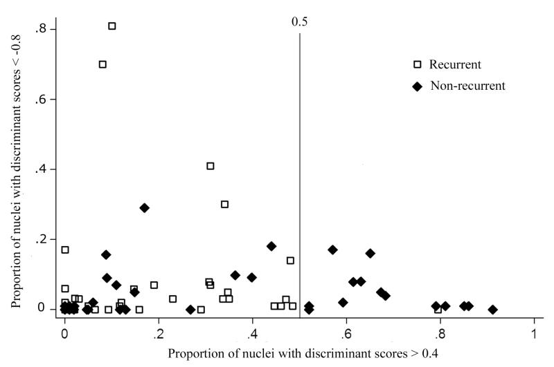
In situations where the distributions of nuclear values for the entire data sets show severe overlap and there is poor prospect for adequate discrimination on that basis, it is sometimes helpful to inspect the score distributions for each case. In this instance, inspection revealed that about one third of the NR cases had a high percentage of nuclei in the high positive score range. In fact, setting a threshold on the DF I,1 axis and using the percent nuclei in each case above that threshold as a “metafeature” allowed a substantial portion of the NR cases to be classified as such without error. This criterion--more than 50% of nuclei above the threshold--was used as a first stage in a hierarchic decision sequence. The cases with that percentage of nuclei above threshold were declared identified as NR and removed from further consideration. A plot was prepared, shown in Fig. 6, with the proportion of nuclei with a discriminant function score less than – 0.8 plotted as ordinate. This did not, however, result in useful information.

Figure 6.

First stage in a hierarchic classification scheme to identify cases with high likelihood for recurrence of papillary bladder cancer. Cases that had more than 50% of their nuclei with a discriminant function score of greater than +0.4 were declared “non-recurrent”.

For all of the remaining cases, a new feature selection was done and a discriminant function DF I,2 was derived. The scores for the DF I,2 function were saved. The primary objective for this was a targeted, more specific feature selection for non-supervised learning processing. The features given the highest weight by the discriminant algorithm were submitted to the non-supervised learning procedure P-index [18, 25].

The rationale for this approach was that the score distribution of the DF I,1 function suggested phenotypical heterogeneity, and that the discriminant function DF I,2 did not result in a useful distinction of R and NR cases. It was hoped that a difference in the composition of subpopulations of different phenotype might allow such a distinction.

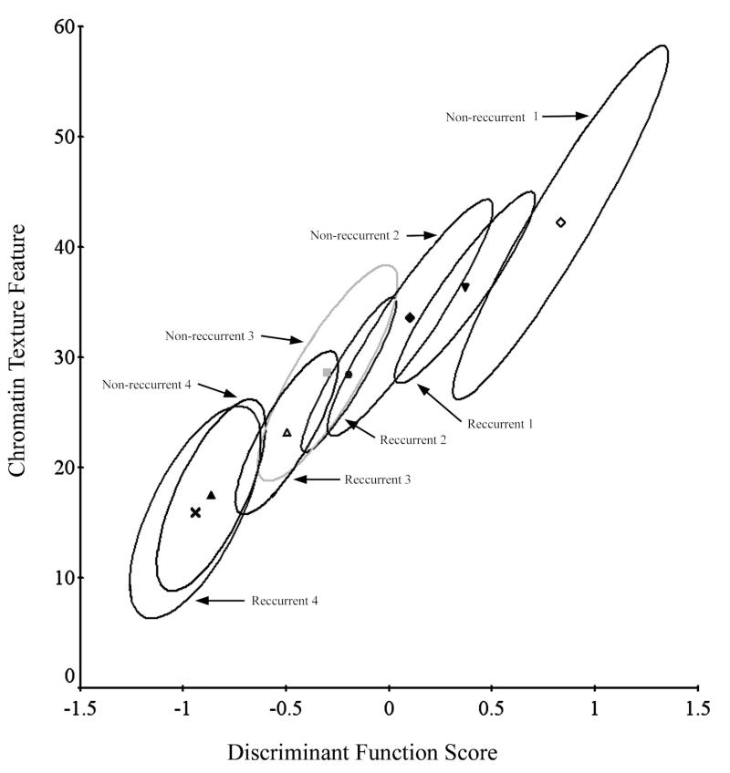
Two runs of that algorithm were set up separately for the NR and the R data sets, based on five features. The P-index algorithm formed four clusters, for each data set (NR and R data sets). The clusters corresponded between the NR and the R data sets in pairs, with a moderate shift of the R clusters away from the corresponding NR clusters. Of the four cluster pairs, one pair at the high end of the feature value range showed non-overlapping confidence ellipses for the nuclei from R and from NR cases. These nuclei were denoted as R1 and NR1. The next cluster pair, NR2 and R2 has overlapping confidence ellipses, but still shows some separation. This offered potential for a diagnostic differentiation. A bivariate plot, based on the DF I,2 score and one of the features used in the non-supervised learning algorithm (a chromatin texture feature) is shown in Fig. 7.

Figure 7.

Processing of the remaining data by the non-supervised learning algorithm P-index. The algorithm formed four clusters each for the recurrent and the non-recurrent cases. The clusters correspond to each other. For the clusters NR1 and R1 a diagnostically useful separation is seen--the prognostically interesting information is expressed in only a subset of the data.

The P-index algorithm computes the mean vector of the employed features and the variance-covariance matrix for each cluster. These data are saved for later use in setting up a classification sequence for an unknown case, as described below.

Nuclei from each case of the NR data set, and of the R data set were assigned if not to all four, at least to one of the clusters. For each cluster, the mean value of the nuclei from each case was computed, since a diagnostic distinction had to result in a case assignment. Four NR and R pairs resulted. First, cases were classified based on the assignment of their nuclei to NR1 or R1 cluster. A record was kept of the cases correctly assigned NR or R categories and of the erroneously assigned cases. The cases thus identified were removed from further consideration (i.e. the mean values of their nuclei were removed from the second cluster pairs NR2 and R2). Then, the process was repeated for the second cluster pair. In this study, no further classification of nuclei assigned to the third and fourth cluster pairs was needed.

The hierarchic classification procedure resulted in the correct identification of 37 of the 40 patients experiencing recurrence, and of 41 of the 45 patients free from recurrence. Thus, for the total of 85 cases there were 92% correct assignments. The discriminating information predicting risk for recurrence was found in the subset of nuclei assigned to the first or second clusters.

Classification procedure for an unknown case

The above sequence is not useful for the processing of a single, unknown new case. To derive a classification procedure for unknown cases, the following procedure sequence was developed. The discriminant function score for DF I,1 is computed, and the percentage of nuclei above the threshold on the score axis is determined. If the percentage is above 50%, the case is classified as non-recurrent. If below 50%, the five features used in the P-index run are computed.

A run of the Cooley-Lohnes maximum likelihood classifier [26] is set up for the features used in the original P-index algorithm for eight classes: four clusters of the R data set and four clusters of the NR data set. For these, the cluster mean vectors and variance-covariance matrices computed by the P-index algorithm were used in the Cooley-Lohnes classification algorithm. Nuclei of the unknown case were classified by the Cooley-Lohnes algorithm on the basis of a maximum likelihood criterion. The mean value for the nuclei from the single, unknown case, in each cluster is computed. The case was assigned based on the classification of its nuclei.

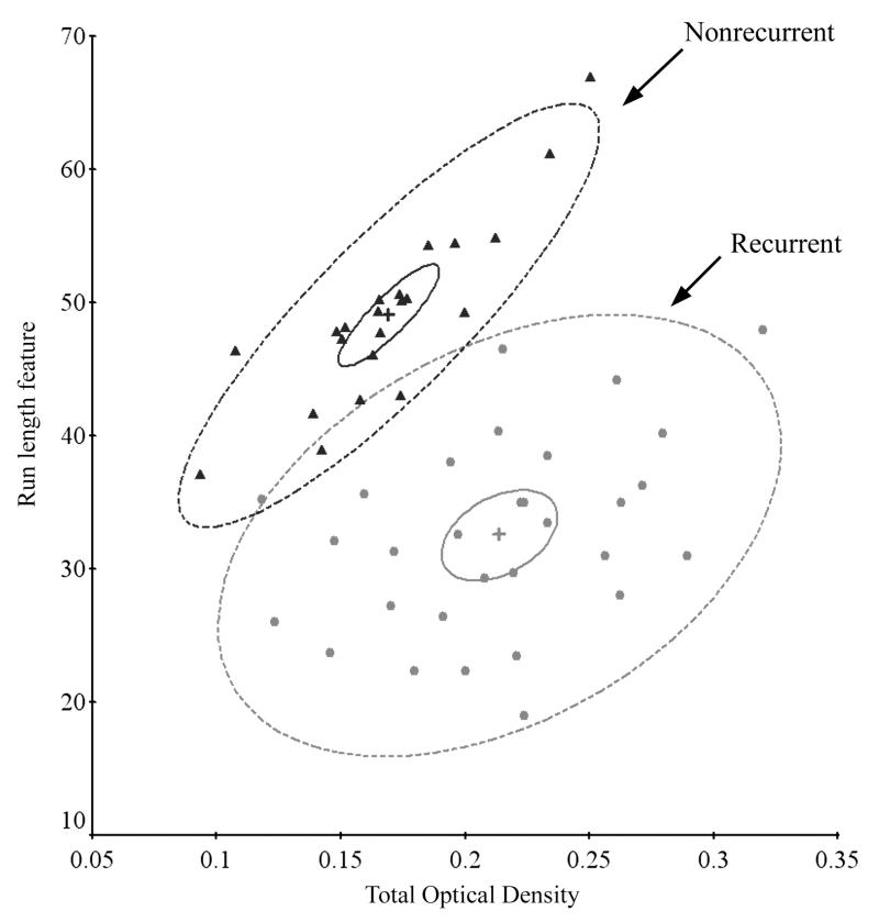
To visualize the results, a bivariate plot was prepared. The P-index algorithm provides a listing of the mean values of the features for each cluster. From this listing two features with the greatest difference in value between clusters for the R and the NR data sets were selected by inspection, to allow a bivariate plot. The mean values of those two features, for each case assigned to either the NR1 or the R1 cluster were plotted, as seen in Fig. 8.

Figure 8.

Classification of individual cases by the Cooley-Lohnes algorithm into clusters NR1 and R1. Shown are the bivariate mean vectors for each case, the 95% confidence ellipses for those mean values, and the 90% tolerance ellipses.

Case study 4: Second order discriminant analysis

In a clinical study of the efficacy of topically applied Vitamin A at various dose levels to prevent actinic damage to the skin [27], biopsies were taken at baseline and at 12 months (end of study). An exploratory discriminant analysis DF I,1 of nuclei from skin with no sun exposure versus nuclei from the sun-exposed forearm revealed substantial differences. The question arose whether the features distinguishing nuclei from those two sites were really the best to detect the small changes expected in sun damaged skin due to the Vitamin A intervention.

The processing sequence therefore began by using the score distribution of the DF I,1 function and setting a threshold. The nuclei with scores above the threshold were taken to represent nuclei with greater sun damage, and those below threshold represented nuclei with less damage. Two data sets were formed of these nuclei. However, this was only done for the purpose of feature selection. A Kruskal Wallis test identified a number of features with statistically significant differences at a level of p < 0.005.

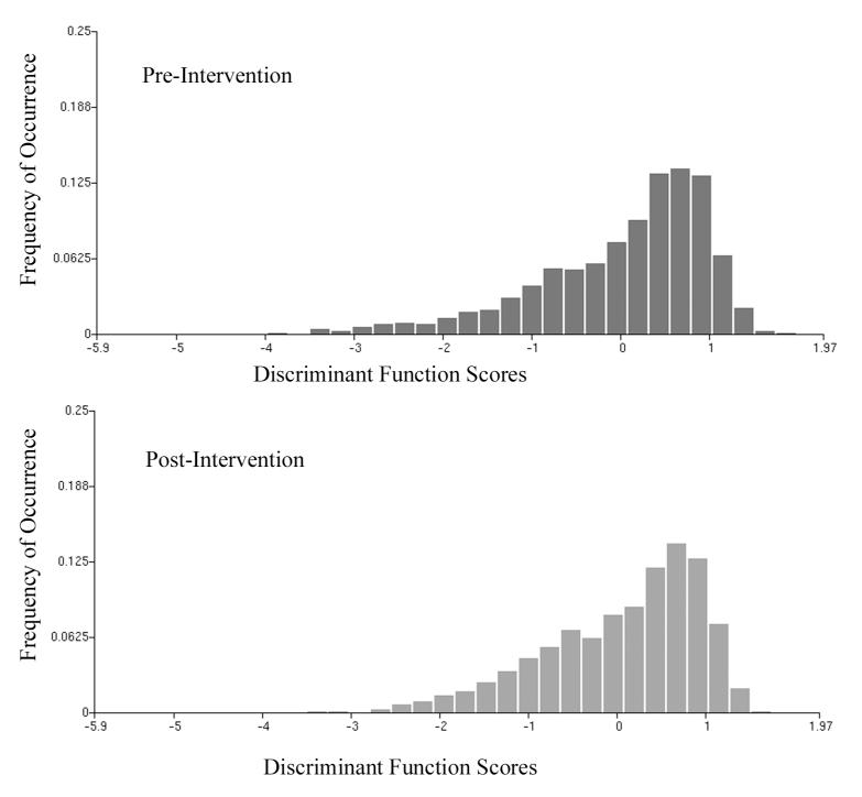
A second discriminant analysis (DF I,2) of the baseline versus the end-of-study data sets was carried out using those features. The score distributions were practically identical, as seen in Fig. 9. There was a very slight shift in the end-of-study distribution towards “less damage”. A threshold was set by visual inspection such that about 15% of nuclei with the highest scores were considered above threshold and excluded. These amounted to 353/2600 nuclei at baseline, but only 258/2600 nuclei at end of study. This reduction in the number of nuclei with higher deviation from normal was statistically significant and an indication that there might be some efficacy of the agent.

Figure 9.

Distribution of discriminant function scores for nuclei from sun-exposed, histologically normal-appearing skin before and after chemopreventive intervention with topically applied Vitamin A. The two distributions are statistically indistinguishable, although there is a very slight shift towards less deviation from normal.

The distributions for the DF I,2 scores of the baseline and end-of-study data were not significantly different according to the Kolmogorov-Smirnoff test [28]. No adequate classification could be obtained for the nuclei, nor did the case mean scores provide a useful classification. The characteristics of the baseline and end-of-study data sets thus offered no hope for proof of efficacy. However, not all of the information offered by the data had been used. The case mean scores had not been sufficient, but they are just one statistic per case. Yet, each case is also characterized by its own score distribution. The frequencies of occurrence of scores offer as many “metafeatures” as there are intervals along the DF 1,2 axis. This is information that had not been considered.

To provide useful metafeatures, the distributions must have an adequate, large sample size. This, fortunately, was the case in the Vitamin A study, with 100 nuclei per case, 26 cases for the baseline data set and 26 cases for the end-of-study data set, for a total of 5,200 nuclei.

To elect to use metafeatures, one does something counterintuitive. One gives up the large number of degrees of freedom provided by the large sample size of nuclei, and is restricted to the much smaller number of degrees of freedom offered by the number of cases. The range of DF I,2 scores was then divided into 20 intervals (thus, 20 potential metafeatures). A Kruskal Wallis test revealed that 12 had statistical significance at p < 0.01.

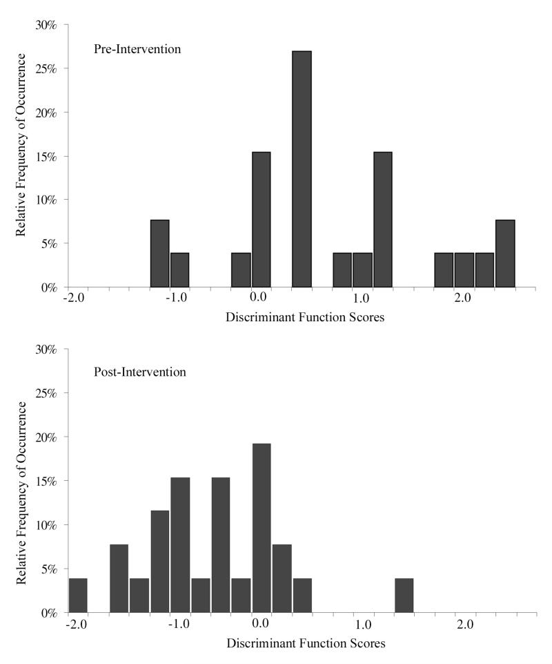
Submitted to a second-order discriminant analysis (DF II,1), the algorithm selected three of the metafeatures. Wilks’ Lambda was reduced to 0.68. The case score distributions for baseline data were correctly identified for 18 of the 26 cases (69%). Twenty-two (22) of 26 (85%) end-of-study cases were correctly identified. The distributions of DF II,1 scores for the 26 cases are shown in Fig. 10.

Figure 10.

Distribution of case scores for the second order discriminant function DF II,1

To secure chemopreventive efficacy by some statistical significance statement several options exist. One may use the discriminant function DF II,1 scores for the 26 cases at baseline and at end of study in an analysis of variance. A randomized block design with pairwise comparison is an appropriate design [29]. This last step in the processing sequence resulted in a significant effect of Vitamin A (p < 0.0001). Between subject variance was not significant.

The above reported results applied to the Vitamin A dose level of 50,000 units over a period of 12 months. In the entire study, patients were randomized to one of four groups--placebo group or one of three treatment groups: 25,000 units; 50,000 units, and 75,000 units of Vitamin A, all of which were analyzed. A dose response curve was constructed using all treatment groups.

Discussion

The rationale for much of the early work in quantitative cytopathology and histopathology was diagnostic decision support [30]. Even then, the use of image information which is either not, or only poorly, visibly appreciated made a valuable contribution. In the great majority of studies, the objective could be accomplished by processing with a single algorithm, such as a straightforward discriminant analysis or a maximum likelihood classifier. This applies even to situations where multiple diagnostic categories had to be considered, and the use of a hierarchic decision sequence was required [31].

In recent years, karyometry has increasingly been applied to problems where visual inspection is entirely equivocal and, where it is not even known a priori, whether diagnostic or prognostic information can be extracted and statistically secured. This is certainly true for the detection of pre-neoplastic lesions, but even more so in efforts to detect very subtle effects due to a chemopreventive intervention, or due to a different risk for lesion recurrence.

The subtle differences that reflect these effects may find expression in value shifts in some features. Although it is not known ahead of time which these might be, they may affect only a small proportion of nuclei, or they may affect only nuclei from a certain phenotype. It may not even be known ahead of time whether such karyometric phenotypes are present or not. Even then, only a proportion of nuclei of a given phenotype may be found to have a nuclear chromatin pattern with measurable differences.

The multivariate statistical analysis algorithms are invaluable in these efforts. However, even advanced multivariate methodology does not offer procedures designed to cope with such data set heterogeneities.

Given the diversity and the expected subtle nature of changes in the nuclear chromatin pattern, it has become clear that a single processing step is unlikely to lead directly to their identification. Instead, processing by a sequence of algorithms, revealing different aspects of the multivariate data sets has been found effective. Some of the processing steps utilize information already and routinely computed in a more exhaustive manner: so the second order discriminant functions or metafeatures in general. Some applications require an iterative approach to arrive at a definition of the most effective features, so e.g. the alternative use of supervised and non-supervised learning algorithms.

Most algorithms are provided by multivariate statistics, but statistical significance is really not the prime reason for their use. Rather, it is their ability to reveal the structure of data sets. It is that structure which allows a biologic interpretation. The material encountered in karyometry has properties which are not usually assumed to be valid in formal statistics. There, variability is attributed to randomness. However, in karyometric data variability may be due not only to randomness, but to the effects of gradual, and different degrees of progression of change within a set of nuclei and, variability is due also to inherent qualitative differences, such as nuclei of different phenotype within the same population of nuclei.

References

- [1].Montironi R, Thompson D,MS, Mazzucchelli R, Peketi P, PW H, et al. Karyometry detects subvisual differences in chromatin organization state between cribriform and flat high-grade prostatic intraepithelial neoplasia. Mod Pathol. 2004;17(8):928–37. doi: 10.1038/modpathol.3800142. [DOI] [PubMed] [Google Scholar]
- [2].Montironi R, Scarpelli M, Mazzucchelli R, Hamilton PW, Thompson D, Ranger-Moore J, et al. Subvisual changes in chromatin organization state are detected by karyometry in the histologically normal urothelium in patients with synchronous papillary carcinoma. Hum Pathol. 2003 Sep;34(9):893–901. doi: 10.1016/s0046-8177(03)00341-1. [DOI] [PubMed] [Google Scholar]
- [3].Palcic B, MacAulay C. Malignancy associated changes: Can they be employed clinically? In: Wied GL, Bartels PH, Rosenthal D, Schenck U, editors. Compendium on thecomputerized cytology and histology laboratory. Tutorials of Cytology; Chicago: 1994. pp. 157–65. [Google Scholar]
- [4].Alberts DS, Einspahr JG, Krouse R, Prasad A, Ranger-Moore J, Hamilton P, Ismail A, Lance MP, Goldschmit S, Hess LM, Yozwiak M, Bartels HG, Bartels PH. Karyometry of the colonic mucosa. Cancer Epidemiol Biomarkers Prev. 2008 doi: 10.1158/1055-9965.EPI-07-0595. in press. [DOI] [PubMed] [Google Scholar]
- [5].Bartels PH, Garcia FAR, Trimble C, Curtin J, Hess LM, Bartels HG, Alberts DS. II: Heterogeneity. 2008. Karyometric assessment of endometrial nuclei from patients with a community diagnosis of atypical endometrial hyperplasia (AEH) Submitted for publication. [Google Scholar]
- [6].Garcia F, Davis J, Alberts DS, Liu Y, Thompson D, Bartels P. A karyometric approach to the characterization of atypical endometrial hyperplasia with and without co-ocurring adenocarcinoma. Anal Quant Ctyol Histol. 2003;25(339-246) [PubMed] [Google Scholar]
- [7].Bozzo P, Alberts DS, Vaught L, da Silva VD, Thompson D, Warneke J, et al. Measurement of chemopreventive efficacy in skin biopsies. Anal Quant Cytol Histol. 2001;23:300–12. [PubMed] [Google Scholar]
- [8].Bartels PH, Fabian CJ, Kimler BF, Ranger-Moore JR, Frank DH, Yozwiak ML, et al. Karyometry of breast epithelial cells acquired by random periareolar fine needle aspiration in women at high risk for breast cancer. Anal Quant Cytol Histol. 2007 Apr;29(2):63–70. [PubMed] [Google Scholar]
- [9].Montironi R, Scarpelli M, Lopez-Beltran A, Mazzucchelli R, Alberts D, Ranger-Moore J, et al. Chromatin phenotype karyometry can predict recurrence in papillary urothelial neoplasms of low malignant potential. Cell Oncol. 2007;29(1):47–58. doi: 10.1155/2007/356464. [DOI] [PMC free article] [PubMed] [Google Scholar]
- [10].Bartels PH, Ranger-Moore J, Alberts D, Hess L, Scarpelli M, Montironi R. Carcinogenesis and the hypothesis of phylogenetic reversion. Anal Quant Cytol Histol. 2006 Oct;28(5):243–52. [PubMed] [Google Scholar]
- [11].Bartels PH, Wied GL. Image analyzing software system for cytology; Proc COMSAC 77, IEEE First International Software and Applications Conference; 1977.pp. 282–4. [Google Scholar]
- [12].Bartels PH, Wied GL. Extraction and evaluation of information from digitized cell images. In: Richmond CR, et al., editors. Mammalian cells: probes and problems. Technical Information Center; Oak Ridge, Tenn: 1975. pp. 15–28. [Google Scholar]
- [13].Young IT, Verbeek PW, Mayall BH. Characterization of chromatin distribution in cell nuclei. Cytometry. 1986 Sep;7(5):467–74. doi: 10.1002/cyto.990070513. [DOI] [PubMed] [Google Scholar]
- [14].Doudkine A, MacAulay C, Poulin N, Palcic B. Nuclear texture measurements in image cytometry. Pathologica. 1995;87:286–99. [PubMed] [Google Scholar]
- [15].Bengtsson E, Nordin B. In: Densitometry, Morphometry and Texture Analysis as Tools in Quantitative Cytometry and Automated Cancer Screening. Grohs H, Husain OAN, editors. 1994. pp. 21–43. [Google Scholar]
- [16].Hastie T, Tibshirani R, Friedman J. The Elements of Statistical Learning : Data mining, Inference, and Prediction. Springer Verlag; New York: 2001. [Google Scholar]
- [17].Fayyad UM, Piatetsky-Shapiro G, Smyth P, Uthurusami R. Advances in Knowledge Discovery and Data Mining. AAAI Press; Menlo Park: 1996. [Google Scholar]
- [18].Bartels PH, Olson GB. Computer analysis of lymphocyte images. In: Catsimpoolas N, editor. Methods of Cell separation. Plenum Press; New York: 1980. pp. 1–99. [Google Scholar]
- [19].Kruskal WH, Wallis WA. Use of ranks on one-criterion variance analysis. J Amer Stat Assoc. 1952;47:583–621. Addendum: 48: 907-11, 1953. [Google Scholar]
- [20].Fleiss J. Statistical methods for rates and proportions. Wiley; New York: 1981. [Google Scholar]
- [21].Alberts DS, Einspahr JG, Krouse R, Prasad A, Ranger-Moore J, Hamilton P, Ismail A, Lance MP, Goldschmit S, Hess LM, Yozwiak M, Bartels HG, Bartels PH. Karyometry of the colonic mucosa. Cancer Epidemiol Biomarkers Prev. 2007;16(12):2704–16. doi: 10.1158/1055-9965.EPI-07-0595. [DOI] [PubMed] [Google Scholar]
- [22].Ranger-Moore J, Alberts DS, Montironi R, Garcia F, Davis J, Frank D, et al. Karyometry in the early detection and chemoprevention of intraepithelial lesions. Eur J Cancer. 2005;41(13):1875–88. doi: 10.1016/j.ejca.2005.07.002. [DOI] [PubMed] [Google Scholar]
- [23].Hartigan B. Clustering algorithms. Wiley; New York: 1975. [Google Scholar]
- [24].Beale EMI. Euclidean cluster analysis. Bull Int Stat Inst. 1969;43(92):21–43. [Google Scholar]
- [25].McClellan RP. Optimization and stochastic approximation techniques applied to unsupervised learning. University of Arizona; Tucson: 1971. [Google Scholar]
- [26].Cooley WW, Lohnes PR. Multivariate Data Analysis. John Wiley; New York: 1971. [Google Scholar]
- [27].Bartels PH, Ranger-Moore J, Stratton MS, Bozzo P, Einspahr J, Liu Y, et al. Statistical Analysis of chemopreventive efficacy of Vitamin A in sun-exposed, normal skin. Anal Quant Cytol Histol. 2002;24(4):185–97. [PubMed] [Google Scholar]
- [28].Kolmogorov A. Confidence limits for an unknown distribution function. Ann Math Statist. 1941;12:461–3. [Google Scholar]
- [29].Sokal RR, Rohlf FJ. Biometry: the principles and practice of statistics in biological research. Freeman; San Francisco: 1969. [Google Scholar]
- [30].Baak JPAaO J. Morphometry in Diagnostic Pathology. Springer Verlag; Berlin: 1983. [Google Scholar]
- [31].Bartels HG, Bartels PH, Bibbo M, Wied GL. Stabilized binary hierarchic classifier in cytopathologic diagnosis. Anal Quant Cytol. 1984;6(4):247–61. [PubMed] [Google Scholar]
- [32].Genchi H, Mori K. Evaluation and feature extraction on automatic pattern recognition system. Denki Tsuchin Gakkai Pari. 1965:1. in Japanese. [Google Scholar]