Estimation of a Multi-fascicle Model from Single B-Value Data with a Population-Informed Prior

Abstract

Diffusion tensor imaging cannot represent heterogeneous fascicle orientations in one voxel. Various models propose to overcome this limitation. Among them, multi-fascicle models are of great interest to characterize and compare white matter properties. However, existing methods fail to estimate their parameters from conventional diffusion sequences with the desired accuracy. In this paper, we provide a geometric explanation to this problem. We demonstrate that there is a manifold of indistinguishable multi-fascicle models for single-shell data, and that the manifolds for different b-values intersect tangentially at the true underlying model making the estimation very sensitive to noise. To regularize it, we propose to learn a prior over the model parameters from data acquired at several b-values in an external population of subjects. We show that this population-informed prior enables for the first time accurate estimation of multi-fascicle models from single-shell data as commonly acquired in clinical context. The approach is validated on synthetic and in vivo data of healthy subjects and patients with autism. We apply it in population studies of the white matter microstructure in autism spectrum disorder. This approach enables novel investigations from large existing DWI datasets in normal development and in disease.

1 Introduction

Diffusion tensor imaging is unable to represent the signal arising from crossing fascicles. Various approaches have been proposed to overcome this limitation. Among them, generative models such as multi-tensor models [2,3] seek to represent the signal contribution from different populations of water molecules. Based on biological modelling, they are of great interest to characterize and compare white-matter properties. However, estimating their parameters from conventional diffusion data has proven inefficient.

Recent works have suggested that part of this inaccuracy is explained by the ill-posedness of the problem and not only by the imaging nuisance [3,4]. To regularize the estimation of models with a single anisotropic tensor, elaborate spatial priors have been proposed [2], and it was shown that acquiring additional b-values improves the analysis of isotropic fraction [1]. For N-tensors, it was proposed to fix the tensor eigenvalues [4], solving the ill-posedness problem but reducing the amount of microstructural information contained in the model. No method has proposed to regularize the estimation of an N-fascicle model while keeping all its degrees of freedom. Furthermore, there is a strong need for a strategy to estimate multi-fascicle models from conventional single-shell data due to their wide availability in clinical setting. Section 2 analyzes the estimation problem from a geometric point of view. Section 3 develops an estimator based on a prior informed by an external population of subjects. Section 4 presents results and Section 5 concludes. Conclusions about estimating an N-tensor model can be applied to all generative models that include a multi-tensor as part thereof.

2 Manifolds of Equivalent Models at a Given B-value

A multi-fascicle model is represented as a mixture of single fascicle models. In the multi-tensor formalism, the generative model for the formation of the diffusion signal S for a b-value b and a gradient direction g is:

$$S=S_0\sum _{i=1}^N{f}_i{e}^{-b{\mathit{g}}^T{\mathit{D}}_i\mathit{g}},$$ (1)

where D_i and f_i are the tensor and the volumetric fraction of fascicle i. Since γ_ie^{−log γ_i}=1, all multi-fascicle models with fractions γ_if_i and tensors ${\mathit{D}}_i+\frac{log{\gamma }_i}{b}\mathit{I}$ produce the same signal:

$$S=S_0\sum _{i=1}^N{\gamma }_i{f}_i{e}^{-b{\mathit{g}}^T\left({\mathit{D}}_i+\frac{log{\gamma }_i}{b}\mathit{I}\right)\mathit{g}},\text{with}\text{the}\text{constraint}\sum _{i=1}^N{\gamma }_i{f}_i=1.$$ (2)

The tensors remain positive definite as long as ${\gamma }_i>e^{-b{\lambda }_i^{min}}$, where ${\gamma }_i^{min}$ is the lowest eigenvalue of D_i. Each of these models is uniquely identified by its vector ( ${\lambda }_1^{min},\dots ,{\gamma }_N^{min}$). The set of all models respecting Equation (2) is a manifold of dimension (N − 1) defined by the implicit equations (we let ${\lambda }_i:={\lambda }_i^{min}$):

$$\{\begin{array}{l}{\lambda }_i={\lambda }_i^{\text{true}}+\frac{1}{b}log({\gamma }_i)\text{for}i=1,\dots ,N\hfill \\ {\sum }_{i=1}^N{\gamma }_i{f}_i=1,\hfill \end{array}$$ (3)

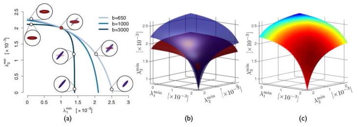
where ( ${\lambda }_1^{\text{true}},\dots ,{\lambda }_N^{\text{true}}$) is the true unknown model (Fig. 1(a)). Since these equations depend on b, so will the manifold. Acquiring diffusion images at different b-values amounts to defining different such manifolds. Let us investigate how those manifolds intersect at the point of interest ${\lambda }_i-{\lambda }_i^{\text{true}}$. The explicit equation of the hypersurface λ_N (λ₁, …, λ_N−1) obtained by eliminating the γ’s between equations (3) is:

$${\lambda }_N({\lambda }_1,\dots ,{\lambda }_{N-1})={\lambda }_N^{\text{true}}+\frac{1}{b}log\left(\frac{1-{\sum }_{i=1}^{N-1}{f}_i{e}^{b({\lambda }_i-{\lambda }_i^{\text{true}})}}{f_N}\right).$$ (4)

Fig. 1.

(a) Infinitely many models produce the same diffusion signal at a given b-value and form a manifold. The manifolds for different b-values intersect at the true underlying model. (b) For N-fascicle models (here N =3), manifolds are (N−1)-dimensional hypersurfaces that intersect tangentially, making the estimation sensitive to noise. (c) The population-informed prior assigns different probabilities to models on the manifold.

The normal vector to the hypersurface is $\mathit{\eta }=\left(\frac{\partial {\lambda }_N}{\partial {\lambda }_1},\dots ,\frac{\partial {\lambda }_N}{\partial {\lambda }_{N-1}},-1\right)$. Its k-th component evaluated at the true model is:

$${{\eta }_k|}_{{\lambda }_i={\lambda }_i^{\text{true}},\forall i}={\frac{\partial {\lambda }_N}{\partial {\lambda }_k}|}_{{\lambda }_i={\lambda }_i^{\text{true}},\forall i}=\frac{-f_k}{f_N}.$$ (5)

Remarkably, this normal vector (and thereby the tangent hyperplane) does not depend on b at the point of interest. In other words, at the first-order approximation, the manifolds at all b-values coincide locally, explaining the high sensitivity to noise encountered when optimizing the parameters of a multi-fascicle model (Fig. 1(b)).

At the second-order approximation, the manifold is characterized by the Hessian matrix of λ_N (λ₁, …, λ_N−1):

$${\mathit{H}|}_{{\lambda }_i={\lambda }_i^{\text{true}}}=\frac{-b}{f_N^2}\left(\stackrel{\sim }{f}{\stackrel{\sim }{f}}^T+f_N\text{diag}(\stackrel{\sim }{f})\right)$$

where f̃ = [f₁, …, f_N−1]^T. The difference between the Hessian matrices at two different b-values, b and b′ > b, is positive definite since, for all x ≠ 0, we have

$$x^T(\mathit{H}(b)-\mathit{H}(b^{\prime }))x=\frac{b^{\prime }-b}{f_N^2}\left({({\stackrel{\sim }{f}}^{T}x)}^2+f_N{x}^T\text{diag}(\stackrel{\sim }{f})x\right)>0.$$ (6)

Therefore, there exists no direction x along which the two manifolds have the same curvature. Consequently, the true model is locally the only intersection of all manifolds. Given the difference (6), it appears that a wider range of b-values leads to a larger difference between their manifolds, which should in turn improve the accuracy of the estimation (ignoring the potential impact of b on noise).

When an isotropic compartment f_isoe^−bD_iso is added to the model, one can show that the above development remains valid with an unchanged N if D_iso is known and considering an (N + 1)-fascicle model if D_iso needs also be optimized.

3 Posterior Predictive Distribution of the Parameters

While all models of (3) are equally compatible with the observed DWI at a given b-value, they are not all as likely from a biological point of view. This knowledge can be learnt from available observations at several b-values of a fascicle i in m_i subjects ${\mathcal{F}}_i=\{f_i^0,\dots ,f_i^{m_i}\},{\mathcal{D}}_i=\{{\mathit{D}}_i^0,\dots ,{\mathit{D}}_i^{m_i}\}$, and incorporated in the estimation as a prior over the parameters (f_i, D_i) (Fig. 1(c)). If the effect of the fascicle properties on partial voluming is negligible, and if the properties of one fascicle are independent of those of another, then the prior can be expressed as:

$$P_{\mathbf{f},\mathbf{D}}(\mathit{f},\mathit{D};\mathit{\theta })=P_{\mathbf{f}}(\mathit{f};{\mathit{\theta }}_f)\prod _{i=1}^N{P}_{{\mathbf{D}}_i}({\mathit{D}}_i;{\mathit{\theta }}_i).$$ (7)

The fractions are not independent since they sum to 1. However, we assume that any fraction f_i is independent of the relative proportions of others f_j/(1 − f_i). This neutral vector assumption naturally leads to the Dirichlet distribution:

$$P_{\mathbf{f}}(\mathit{f};\mathit{\alpha })=\frac{{𝟙}_{\mathit{f}\in \mathcal{S}}}{B(\mathit{\alpha })}\prod _{i=1}^N{f}_i^{{\alpha }_i-1},\text{where}\mathcal{S}=\left\{\mathit{x}\in {ℝ}^N:x_i>0,\sum _{i=1}^N{x}_i=1\right\}.$$ (8)

To prevent negative eigenvalues of the tensors, the prior knowledge about D_i can be described as a multivariate Gaussian distribution over their logarithm [5]:

$${\mathbf{L}}_i=log{\mathbf{D}}_i~\mathcal{N}({\mathbf{M}}_i,{\mathit{\sum }}_i).$$ (9)

In general, Σ_i has 21 free parameters, which may overfit the usually small training dataset. For DTI, it is suggested in [5] to constrain Σ_i to be orthogonally invariant, imposing the following structure that depends only on σ_i and ι_i:

$${\mathit{\sum }}_i={\sigma }_i^2\left(\begin{array}{cc}{I}_3+\frac{{\tau }_i}{1-3{\tau }_i}{𝟙}_3& \mathbf{0}\\ \mathbf{0}& I_3\end{array}\right)\triangleq \mathit{B}({\sigma }_i,{\tau }_i).$$

This structure yields a closed-form solution for the maximum likelihood [5]:

$${\widehat{\mathit{M}}}_i={\overline{\mathit{L}}}_i=\frac{1}{m_i}\sum _{k=1}^{m_i}{\mathit{L}}_i^k\text{and}{\widehat{\mathit{\sum }}}_i=\mathit{B}({\widehat{\sigma }}_i,{\widehat{\tau }}_i),$$ (10)

$$\text{with}{\widehat{\tau }}_i=\frac{-{\sum }_{i=1}^{m_i}{\Vert {\mathit{L}}_i^k-{\overline{\mathit{L}}}_i\Vert }_2^2}{5{\sum }_{i=1}^{m_i}{\left[\text{Tr}({\mathit{L}}_i^k-{\overline{\mathit{L}}}_i)\right]}^2}\text{and}{\widehat{\sigma }}_i^2=\frac{1}{6m_i}\sum _{i=1}^{m_i}{\Vert {\mathit{L}}_i^k-{\overline{\mathit{L}}}_i\Vert }_{{\widehat{\tau }}_i}^2,$$ (11)

where ${\Vert .\Vert }_t^2$ is defined by 〈A, B〉_t=Tr(AB)−t Tr(A)Tr(B). The ML estimator may be unreliable for compartments with only a few observations. This uncertainty is accounted for by replacing point estimates of θ by posterior distributions and integrating over all possible θ. This yields the posterior predictive distribution (PPD) which contains all the knowledge about new observations that we learn from previous observations. Its derivation requires the definition of hyperpriors over θ and is closed-form if we select conjugate hyperpriors. M_i ~ (M₀, Λ₀) is a conjugate hyperprior for the tensor part of (7) assuming a deterministic Σ_i = Σ̂ _i. We set Λ₀=B(1, 0) and M₀=log D_iso to keep it weakly informative (this hyperprior merely encodes the order of magnitude of diffusivity at 37°C). The PPD over the tensors is ${\mathit{D}}_i\mid {\mathcal{D}}_i~\mathcal{N}({\mathit{M}}_i^{m_i},{\mathit{\Lambda }}_i^{m_i})$ with

$${\mathit{\Lambda }}_i^{m_i}={\widehat{\mathit{\sum }}}_i+{\left({\mathit{\Lambda }}_0^{-1}+m_i{{\widehat{\mathit{\sum }}}_i}^{-1}\right)}^{-1}\triangleq \mathit{B}({\stackrel{\sim }{\sigma }}_i,{\stackrel{\sim }{\tau }}_i),$$ (12)

$$\text{and}{\mathit{M}}_i^{m_i}={\left({\mathit{\Lambda }}_0^{-1}+m_i{{\widehat{\mathit{\sum }}}_{\mathit{i}}}^{-1}\right)}^{-1}\left({\mathit{\Lambda }}_0^{-1}{\mathit{M}}_0+m_i{{\widehat{\mathit{\sum }}}_{\mathit{i}}}^{-1}{\overline{L}}_i\right).$$ (13)

For the parameters α_i, a conjugate hyperprior is the Dirichlet distribution. We set all its parameters to 1, making it uniform over the simplex . The resulting PPD is a Dirichlet with parameters $1+{\sum }_{k=1}^{m_i}{f}_i^k$. In this expression, we consider $f_i^k$ as frequency counts since they are samples of f_i rather than samples from a multinomial parameterized by f_i. The complete PPD is (with constant):

$$P_{\mathbf{f},\mathbf{D}}(\mathit{f},\mathit{D}\mid \mathcal{F},\mathcal{D})=C_{\mathcal{F},\mathcal{D}}{𝟙}_{\mathit{f}\in \mathcal{S}}\prod _{i=1}^N{f}_i^{{\sum }_{k=1}^{m_i}{f}_i^k}\prod _{i=1}^{N}exp\left\{-\frac{{\Vert {\mathit{L}}_i-{\mathit{M}}_i^{m_i}\Vert }_{{\stackrel{\sim }{\tau }}_i}^2}{2{\stackrel{\sim }{\sigma }}_i^2}\right\}.$$ (14)

We incorporate this PPD as a prior in the estimation. We assume Gaussian noise on the DWI measurements y_k since they are acquired on a single shell typically at b=1000 for which noise is approximately Gaussian. The maximum a posteriori estimator at each voxel amounts to maximizing the following for f and D:

$$L=log({𝟙}_{\mathit{f}\in \mathcal{S}})+\sum _{i=1}^N\sum _{k=1}^{m_i}{f}_i^k{f}_i-\sum _{i=1}^N\frac{{\Vert {\mathit{L}}_i-{\mathit{M}}_i^{m_i}\Vert }_{{\stackrel{\sim }{\tau }}_i}^2}{2{\stackrel{\sim }{\sigma }}_i^2}-\sum _{k=1}^K\frac{{(S_k(\mathit{f},\mathit{D})-y_k)}^2}{2{\sigma }_k^2}.$$ (15)

The influence of the noise ${\sigma }_k^2$ is analyzed in the next section. In practice, the prior is built from data acquired in completely different subjects at several b-values. All these subjects are registered to a multi-fascicle atlas as in [7]. Following alignment, tensors from all subjects at each voxel are clustered in N compartments as in [6]. Each cluster represents the sets and of available observations. The prior is then aligned with an initial estimate (without prior) of the multi-fascicle model. To evaluate (14), all assignments of compartments to tensors are considered and the highest prior value is recorded. BOBYQA algorithm is used to maximize (15) and the number of fascicles is estimated by an F-test as in [3].

4 Results

We compare the models estimated by our method to a ground truth {g_i, G_i} with five root mean square metrics, Δ_FA, Δ_MD, Fro, Δ_F and Δ_iso defined by:

$$\begin{array}{l}{\mathrm{\Delta }}_{\text{FA}}^2=\sum _{i=1}^N\frac{f_i+g_i}{2}{(\text{FA}({\mathit{F}}_i)-\text{FA}({\mathit{G}}_i))}^2,{\mathrm{\Delta }}_{\text{MD}}^2=\sum _{i=1}^N\frac{f_i+g_i}{2}{(\text{MD}({\mathit{F}}_i)-\text{MD}({\mathit{G}}_i))}^2\\ {\text{Fro}}^2=\sum _{i=1}^N\frac{f_i+g_i}{2}{\Vert {\mathit{D}}_i-{\mathit{G}}_i\Vert }_F,{\mathrm{\Delta }}_{\mathrm{F}}^2=\sum _{i=1}^N{(f_i-g_i)}^2\text{and}{\mathrm{\Delta }}_{\text{iso}}^2={(f_{\text{iso}}-g_{\text{iso}})}^2.\end{array}$$

Synthetic Phantom Experiment

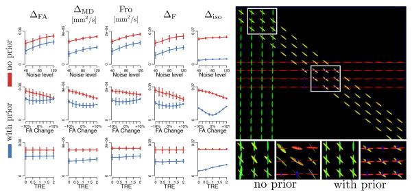
DWI were simulated under Rician noise from a phantom containing an isotropic compartment and 0 to 3 tensors of various properties with S₀=400. The prior was built from 20 datasets of 90 DWI at b=1000, 2000 and 3000. The accuracy was evaluated with 20 datasets of 30 DWI at b=1000 in three scenarios. First, the noise variance increased from 40 to 120. Second, the FA of the phantom was offset by −10% to +10% without changing the prior to simulate patient’s data with a prior built from healthy subjects. Third, random deformations of 0 to 2 voxels were applied to the prior to simulate registration errors. In the last two scenarios, the noise variance was 80. In all scenarios and for all metrics, incorporating the prior significantly improved the accuracy of the estimation (one-tail paired t-test: p < 10⁻⁶) (Fig. 2)

Fig. 2.

(Left) Incorporating the prior in the estimation significantly improves the accuracy of the estimated model under the three simulated scenarios and for all five comparison metrics (distributions are shown for 20 datasets simulated for each set of parameters).(Right) The better accuracy mostly affects the diffusion properties of tensors (other than their directions), as predicted by Equation (3).

In Vivo Data Experiment

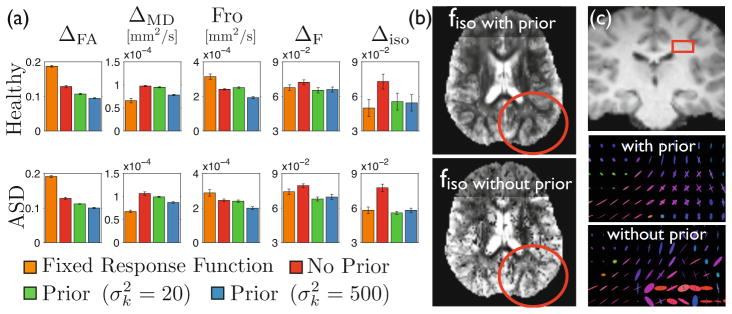
Eighteen healthy subjects and 10 subjects with autism were imaged to test the method and an extra 13 healthy subjects were imaged to build the prior. For all subjects, DWI at resolution 1.7 × 1.7 × 2mm³ were acquired with a Siemens 3T Trio with a 32 channel head coil using the CUSP-45 sequence [3]. This includes 30 gradients on a single-shell at b = 1000 and 15 gradients with b-values up to 3000. For each test subject, all 45 DWI were first used to estimate a multi-fascicle model considered as a ground truth. Estimations using the single-shell subset only were then compared to it. Four strategies were compared: estimation without prior, estimation by fixing all tensors to a globally optimized value, and estimation with the prior assuming a noise level ${\sigma }_k^2$ of 20 and 500. Results in Fig. 3 show that estimations which incorporate a prior outperform other strategies. Estimations with ${\sigma }_k^2=500$ are significantly better than estimations without prior for all metrics and, remarkably, for both healthy controls and ASD patients (one-tail paired t-test: p < 10⁻⁶). The true noise level of DWI is arguably closer to 500 than 20. However, estimations with ${\sigma }_k^2=20$ remain more accurate than estimations without prior, indicating that the population-informed prior improves the model accuracy even for crude estimates of the noise level. Empirical estimates of this noise level is kept for future work. Finally, fixing the fascicle response results in accuracies that strongly vary among quality metrics and, furthermore, only provides average information about the brain microstructure, which is not suitable in most studies.

Fig. 3.

(a) Incorporating prior knowledge significantly improves the quality of the model estimation for all five metrics and for both healthy controls and ASD patients. This improvement implies that (b) the extracellular water fraction can be visualized with more contrast and less noise in smaller details of the white matter up to its boundary with the grey matter, and (c) properties of the fascicles in crossing areas (shown is the corona radiata) are better represented and do not suffer the arbitrary choice of a model from Equation (3).

Application to Population Studies

One could be concerned that the improved accuracy brought by the prior would come with a severe shrinkage of the estimated parameters towards the mean of the population. This would prevent its use in population studies. To address this concern, we conducted two population studies of autism spectrum disorder (ASD) using the proposed estimator. The first one focused on fascicle properties in the left arcuate fasciculus by analyzing the FA along the median tract. The second study investigated whether an increased extracellular volume fraction f_iso is observed in ASD. Less restricted diffusion may be related to the presence of edema, thinner axons, and neuroinflammation [1]. The latter has been proposed as a possible cause of autism. Corrections for multiple comparisons were based on cluster-size statistics in 1000 permutations with a threshold on t-scores of 3. As presented in Fig. 4, the first study revealed decreased FA integrity in the arcuate fasciculus of patients with ASD, in line with most recent studies of autism. The second study revealed one clusters of significantly increased unrestricted diffusion (permutation test: p < 0.003). Without the prior, none of these findings were observed (p > 0.1). These studies show that the use of a prior in the estimation preserves contrasts of diffusion properties between groups, so that single-shell HARDI data can be used in large population studies based on multi-fascicle models.

Fig. 4.

The population-informed prior enables population studies of multi-fascicle models from single-shell HARDI data. (a–b) The first study reveals significantly decreased FA related to autism in the left arcuate fasciculus (*p<.05,**p<.01). (c–d) The second study reveals a cluster of significantly higher f_iso. (d) Average f_iso in the cluster.

5 Conclusion

Multi-fascicle models cannot be estimated from conventional single-shell HARDI data because a manifold of models produce the same diffusion signals. However, we showed that a posterior predictive distribution over the model parameters can be learnt from data acquired at several b-values in an external population. By incorporating this population-informed prior in the maximum a posteriori estimator of the parameters, we are able to estimate accurate multi-fascicle models from data at a single b-value. This method thus opens new opportunities for population studies with the large number of available clinical diffusion images.

References

- 1.Pasternak O, Shenton ME, Westin C-F. Estimation of extracellular volume from regularized multi-shell diffusion MRI. In: Ayache N, Delingette H, Golland P, Mori K, editors. MICCAI 2012, Part II. LNCS. Vol. 7511. Springer; Heidelberg: 2012. pp. 305–312. [DOI] [PMC free article] [PubMed] [Google Scholar]
- 2.Pasternak O, Sochen N, Gur Y, Intrator N, Assaf Y. Free water elimination and mapping from diffusion MRI. Magnet Reson Med. 2009;62(3):717–730. doi: 10.1002/mrm.22055. [DOI] [PubMed] [Google Scholar]
- 3.Scherrer B, Warfield SK. Parametric representation of multiple white matter fascicles from cube and sphere diffusion MRI. PLoS one. 2012;7(11):e48232. doi: 10.1371/journal.pone.0048232. [DOI] [PMC free article] [PubMed] [Google Scholar]
- 4.Schultz T, Westin C-F, Kindlmann G. Multi-diffusion-tensor fitting via spherical deconvolution: a unifying framework. In: Jiang T, Navab N, Pluim JPW, Viergever MA, editors. MICCAI 2010, Part I. LNCS. Vol. 6361. Springer; Heidelberg: 2010. pp. 674–681. [DOI] [PMC free article] [PubMed] [Google Scholar]
- 5.Schwartzman A, Mascarenhas WF, Taylor JE. Inference for eigenvalues and eigenvectors of gaussian symmetric matrices. Ann Stat. 2008:2886–2919. [Google Scholar]
- 6.Taquet M, Scherrer B, Benjamin C, Prabhu S, Macq B, Warfield S. Interpolating multi-fiber models by gaussian mixture simplification. IEEE ISBI. 2012:928–931. [Google Scholar]
- 7.Taquet M, Scherrer B, Commowick O, Peters J, Sahin M, Macq B, Warfield SK. Registration and analysis of white matter group differences with a multi-fiber model. In: Ayache N, Delingette H, Golland P, Mori K, editors. MICCAI 2012, Part III. LNCS. Vol. 7512. Springer; Heidelberg: 2012. pp. 313–320. [DOI] [PMC free article] [PubMed] [Google Scholar]