

Abstract
This paper investigates an approach to model the space of brain images through a low-dimensional manifold. A data driven method to learn a manifold from a collections of brain images is proposed. We hypothesize that the space spanned by a set of brain images can be captured, to some approximation, by a low-dimensional manifold, i.e. a parametrization of the set of images. The approach builds on recent advances in manifold learning that allow to uncover nonlinear trends in data. We combine this manifold learning with distance measures between images that capture shape, in order to learn the underlying structure of a database of brain images. The proposed method is generative. New images can be created from the manifold parametrization and existing images can be projected onto the manifold. By measuring projection distance of a held out set of brain images we evaluate the fit of the proposed manifold model to the data and we can compute statistical properties of the data using this manifold structure. We demonstrate this technology on a database of 436 MR brain images.
1 Introduction
Recent research in the analysis of populations of brain images shows a progression: from single templates or atlases [1], to multiple templates or stratified atlases [2], mixture models [3] and template free methods [4–6] that rely on a sense of locality in the space of all brains. This progression indicates that the space of brain MR images has a structure that might also be modeled by a relatively low-dimensional manifold as illustrated by Figure 1. The aim of this paper is to develop and demonstrate the technology to learn the manifold structure of sets of brain MR images and to evaluate how effective the learned manifold is at capturing the variability of brains.
Fig. 1.
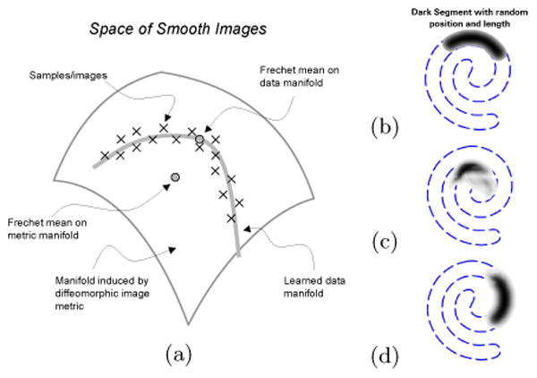
(a) Illustration of image data on a low-dimensional manifold embedded in a diffeomorphic space. (b) A set of images consists of random length/position segments form a spiral. (c) The Fréchet mean in the diffeomorphic space is not like any example from the set. (d) Fréchet mean on data-driven manifold reflects the image with average parameter values.
Manifold learning [7] refers to the task of uncovering manifolds that describe scattered data. In some applications this manifold is considered a generative model, analogous to a Gaussian mixture model. In this context, we assume that the data is sampled from a low-dimensional manifold embedded in a high-dimensional space, with the possibility of noise that sets data off the surface. For this work, we consider the space of all images which can be represented as smooth functions. Virtually all manifold learning techniques published to date assume that the the low-dimensional manifold is embedded in a Euclidean space. Nearby samples lie in the tangent space of the manifold, and thus their differences can be evaluated by Euclidean distance in the ambient space. The space of brain images on the other hand does not fit directly into this paradigm. A great deal of research on brain image analysis shows that the L2 distance is not suitable for measuring shape changes in images [8], but that the metric for comparing brain images should account for deformations or shape differences between images. For example, computational anatomy, used for population analysis and atlas building, is based on a metric between images derived from coordinate transformations [2, 9, 3].
The low-dimensional manifold of brain images we aim to learn is embedded not in Euclidean space, but in the space of images with a metric based on coordinate transformations. For this work we adapt the image metric based on diffeomorphic coordinate transformations [10–12] to manifold learning. Often the stratification induced by the diffeomorphic image metric is described as a manifold—in this paper we refer to the manifold of brain images as described by the data. Our hypotheses are that the space of brain images is some very small subspace of images that are related by diffeomorphisms, that this subspace is not linear, and that we can learn some approximation of this space through a generalization of manifold learning that accounts for these diffeomorphic relationships. Figure 1 illustrates these concepts on a simple example.
A manifold learning algorithm of particular interest to this work is isomap [13]. Isomap is based on the idea of approximating geodesic distances by the construction of piecewise linear paths between samples. The paths are built by connecting nearest neighbors, and the geodesic distance between two points is approximated on the the linear segments between nearest neighbors. Thus, isomap requires only distances between nearby data points to uncover manifold structure in data sets. The reliance on only nearest neighbor distances is important for this paper. The tangent space to the space of diffeomorphic maps is the set of smooth vector fields. Thus, if the samples from the manifold are sufficiently dense, we can compute the distances in this tangent space, and we need only to compute elastic deformations between images.
Isomap, and several other manifold learning algorithms, assign parameters to data points that represent coordinates on the underlying manifold. This paper introduces several extensions to this formulation, which are important for the analysis of brain images. First is an explicit representation of the manifold in the ambient space (the space of smooth functions). Thus, given coordinates on the manifold, we can construct brain images that correspond to those coordinates. We also introduce a mechanism for mapping previously unseen data into the manifold coordinate system. These two explicit mappings allow to project images onto the manifold. Thus we can measure the distance from each image to the manifold (projected image) and quantitatively evaluate the efficacy of the learned manifold. In comparison with previous work, on brain atlases for example, this work constructs, from the data itself, a parametrized hyper-surface of brain images, which represents a local atlas for images that are nearby on the manifold.
2 Related Work
The tools for analyzing or describing sets of brain image demonstrate progressively more sophisticated models. For instance, unbiased atlases are one mechanism for describing a population of brains [14–16]. Blezek et al. [2] propose a stratified atlas, in which they use the mean shift algorithm to obtain multiple templates and shows visualizations that confirm the clusters in the data. In [3] the OASIS brain database is modeled through a mixture of Gaussians. The means of the Gaussians are a set of templates used to describe the population. Instead of assuming that the space of brain images forms clusters, we postulate that the space of brains can be captured by a continuous manifold.
An important aspect of our work is the ability to measure image differences in a way that captures shape. It is known that the L2 metric does not adequately capture shape differences [8]. There are a variety of alternatives, most of which consider coordinate transformations instead of, or in addition to, intensity differences. A large body of work [10–12] has examined distances between images based on high-dimensional image warps that are constrained to be diffeomorphisms. This metric defines a infinite dimensional manifold consisting of all shapes that are equivalent under a diffeomorphism. Our hypothesis, however, is that the space of brains is essentially of significantly lower dimension.
Several authors [17, 9, 6] have proposed kernel-based regression of brain images with respect to an underlying parameter, such as age. The main distinction of the work in this paper is that the underlying parametrization is learned from the image data. Our interest is to uncover interesting structures from the image data and sets of parameters that could be compared against underlying clinical variables.
Zhang et al. use manifold learning, via isomap, for medical image analysis, specifically to improve segmentation in cardiac MR images [18]. Rohde et al. [19] use isomap in conjunction with large deformation diffeomorphisms to embedded binary images of cell nuclei in a similar fashion to the proposed approach. In addition to the embedding we provide a generative model that allows to quantitatively evaluate the manifold fit.
3 Formulation
We begin with a description of the image metric between nearest neighbors in the space of smooth images. A diffeomorphic coordinate transformation between two images is ϕ(x, 1), where , and υ(x,t) is a smooth, time varying vector field. The diffeomorphic framework includes a metric on the diffeomorphic transformation which induces a metric d between images yi and yj:
| (1) |
The metric prioritizes the mappings and, with an appropriate choice of the differential operator L in the metric, ensures smoothness. We introduce the constraint that the transformation must provide a match between the two images:
| (2) |
where ε allows for noise in the images.
For two images that are very similar, ϕ and υ are small, and because the velocities of the geodesics are smooth in time [20], we can approximate the integrals for the coordinate transform and geodesic distance:
| (3) |
Thus, for small differences in images the diffeomorphic metric is approximated by a smooth displacement field. In this paper we use the operator L = αI + ∇, where α is a free parameter and the resulting metric is ∥υ(x)∥L = ∥Lυ(x)∥2. To minimize deformation metric for a pair of discrete images, we use a gradient descent. The first variation of (3) results in a partial differential equation, which we solve with finite forward differences to an approximate steady state. For the constraint, we introduce a penalty on image residual with an additional parameter λ, which we tune in steady state until the residual condition in (2) is satisfied or until the deformation metric exceeds some threshold that disqualifies that pair of images as nearest neighbors. We use a multiresolution, coarse to fine, optimization strategy to avoid local minima.
Next we present a formulation for representing the structure of the manifold in the ambient space and for mapping unseen data onto this intrinsic coordinate system. First, we propose the construction of an explicit mapping f :
 →
→
 from the space of manifold parameters
to the high dimensional ambient space
. Let X = {x1, …, xn} be the parameter values assigned to the image data sets Y = {y1, …, yn}; isomap gives the discrete mapping xi = ρ(yi). Inevitably there will be a distribution of brain images away from the manifold, and the manifold should be the expectation [21] of these points in order to alleviate noise and capture the overall trend in the data. That is f(x) = E(Y |ρ(Y ) = x). In the discrete setting the conditional expectation can be approximated with Nadaraya-Watson kernel regression:
from the space of manifold parameters
to the high dimensional ambient space
. Let X = {x1, …, xn} be the parameter values assigned to the image data sets Y = {y1, …, yn}; isomap gives the discrete mapping xi = ρ(yi). Inevitably there will be a distribution of brain images away from the manifold, and the manifold should be the expectation [21] of these points in order to alleviate noise and capture the overall trend in the data. That is f(x) = E(Y |ρ(Y ) = x). In the discrete setting the conditional expectation can be approximated with Nadaraya-Watson kernel regression:
| (4) |
which we compute, in the context of diffeomorphic image metrics using the method of [9], which iteratively updates f(x) and the deformation to f(x) from the nearest neighbors starting with identity transformations. This kernel regression requires only the nearest neighbors Xnn(x) of xi ∈ X. This constrains the regressions to images similar in shape since locality in X implies locality in Y. Using this formulation, we can compute an image for any set of manifold coordinates, and thus we have an explicit parametrization of the manifold.
For the assignment of manifold parameters to new, unseen images we use the same strategy. We represent this mapping as a continuous function on the ambient space, and we compute it via a regression on parameters given by isomap
| (5) |
with Ynn(y) the nearest neighbors of y. The projection of a new image onto the manifold is the composition of these mappings p(y) = f(ρ′(y)).
For K we use a Gaussian kernel for the mappings with a bandwidth selected based on average nearest neighbor distances. The number of nearest neighbors for the regression is selected based on the resulting bandwidth for the kernel K, such that all points within three standard deviations are included.
4 Results
In section 1 we illustrated the idea of the paper on a simple examples on 2D images of spiral segments. The image data set used consists of 100 images of segments with varying length and location of the spiral in Figure 1. Figure 2 shows images constructed by the proposed approach by sampling the learned manifold representation of the image data. Thus the images depict samples on the manifold embedded in the ambient space. Figure 1 also shows the Fréchet means for the diffeomorphic space and for the manifold learned from the data.
Fig. 2.

Reconstructed images along the first dimension of the manifold learned from spiral segments as illustrated in Figure 1.
We apply the proposed approach to the open access series of imaging studies (OASIS) cross-sectional MRI data set. The images are gain-field corrected and atlas registered. We use 380 of the 436 images to learn the manifold and evaluate reconstruction errors on the left out 56 images.
Figure 3 (a) shows axial slice 80 for a 2D parametrization (manifold coordinates) obtained by the proposed method. A visual inspection reveals that the learned manifold detects the change in ventricle size as the most dominant parameter (horizontal axis). It is unclear if the second dimension (vertical axis) captures a global trend. Figure 3 (b) shows reconstruction errors on the held out images against the dimensionality of the learned manifold. The reconstruction error is measured as the mean of the distances between the original brain images and their projection on to the learned manifold scaled by the average nearest neighbor distance, i.e. . The reconstruction errors are smaller than the average one nearest neighbor distance. An indication that the learned manifold accurately captures the data. The reconstruction errors suggest that the data set can be captured by a 3D manifold. We do not postulate that the space of brains is captured by a 3D manifold. The approach learns a manifold from the available data and thus it is likely that given more samples we can learn a higher dimensional manifold for the space of brains.
Fig. 3.
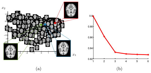
(a)2D parametrization of OASIS brain MRI. The insets show the mean (green), median (blue) and mode (red) of the learned manifold and the corresponding reconstructed images. (b) Reconstruction errors against manifold dimensionality.
Figure 4 shows axial slices of brain images generated with the proposed method on a regularly sampled grid on the 2D representation shown in figure 3(c), i.e. we have sampling of the learned brain manifold. The first dimension (x1) clearly shows the change in ventricle size. The second dimension (x2) is less obvious. A slight general trend observable from the axial slices seems to be less gray and white matter as well as a change in lateral ventricle shape (from elongated to more circular).
Fig. 4.
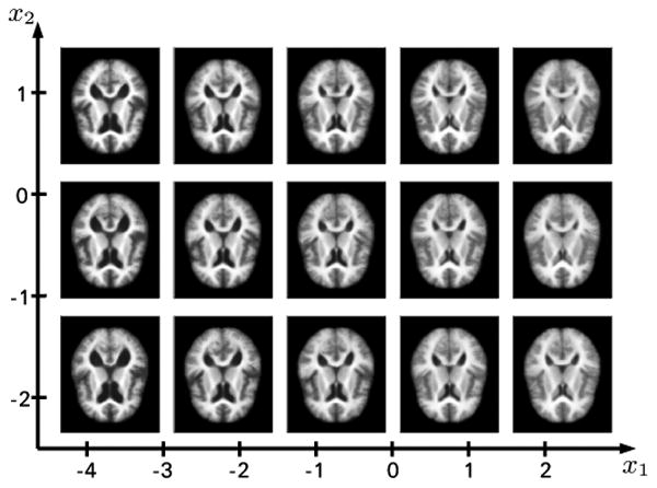
Reconstructions on a grid on the 2D representation shown in figure 3(c).
The method is computationally expensive because of the pairwise distance computations, each requiring an elastic image registration. The registration takes with our multiresolution implementation about 1 minute on a 128 × 128 × 80 volume. Pairwise distances computations for the OASIS database running on a cluster of 50, 2Ghz processors, requires 3 days. The reconstruction by manifold kernel regressions requires about 30 minutes per image on a 2 Ghz processor.
5 Conclusions
Quantitative evaluation illustrates that the space of brains can be modeled by a low dimensional manifold. The manifold representation of the space of brains can potentially be useful in wide variety of applications. For instance, regression of the parameter space with clinical data, such as MMSE or age, can be used to aid in clinical diagnosis or scientific studies. An open question is whether the manifolds shown here represent the inherent amount of information about shape variability in the data or whether they reflect particular choices in the proposed approach. In particular implementation specific enhancements on image metric, reconstruction, and manifold kernel regression could lead to refined results.
Acknowledgments
This work was supported by the NIH/NCBC grant U54-EB005149, the NSF grant CCF-073222 and the NIBIB grant 5RO1EB007688-02.
References
- 1.Woods RP, Dapretto M, Sicotte NL, Toga AW, Mazziotta JC. Creation and use of a talairach-compatible atlas for accurate, automated, nonlinear intersubject registration, and analysis of functional imaging data. Human Brain Mapping. 1999;8(2-3):73–79. doi: 10.1002/(SICI)1097-0193(1999)8:2/3<73::AID-HBM1>3.0.CO;2-7. [DOI] [PMC free article] [PubMed] [Google Scholar]
- 2.Blezek DJ, Miller JV. Atlas stratification. Medical Image Analysis. 2007;11(5) doi: 10.1016/j.media.2007.07.001. [DOI] [PMC free article] [PubMed] [Google Scholar]
- 3.Sabuncu MR, Balci SK, Golland P. Discovering modes of an image population through mixture modeling. MICCAI. 2008;(2):381–389. doi: 10.1007/978-3-540-85990-1_46. [DOI] [PMC free article] [PubMed] [Google Scholar]
- 4.Zöllei L, Learned-Miller E, Grimson E, Wells W. Efficient population registration of 3d data. ICCV. 2005;3765:291–301. of LNCS. [Google Scholar]
- 5.Studholme C, Cardenas V. A template free approach to volumetric spatial normalization of brain anatomy. Pattern Recogn Lett. 2004;25(10):1191–1202. [Google Scholar]
- 6.Ericsson A, Aljabar P, Rueckert D. Construction of a patient-specific atlas of the brain: Application to normal aging. ISBI. 2008 May;:480–483. [Google Scholar]
- 7.Lee JA, Verleysen M. Nonlinear Dimensionality Reduction. Springer; 2007. [DOI] [PubMed] [Google Scholar]
- 8.Twining CJ, Marsland S. Constructing an atlas for the diffeomorphism group of a compact manifold with boundary, with application to the analysis of image registrations. J Comput Appl Math. 2008;222(2):411–428. [Google Scholar]
- 9.Davis BC, Fletcher PT, Bullitt E, Joshi S. Population shape regression from random design data. ICCV. 2007 [Google Scholar]
- 10.Christensen GE, Rabbitt RD, Miller MI. Deformable Templates Using Large Deformation Kinematics. IEEE Transactions on Medical Imaging. 1996;5(10) doi: 10.1109/83.536892. [DOI] [PubMed] [Google Scholar]
- 11.Dupuis P, Grenander U. Variational problems on flows of diffeomorphisms for image matching. Q Appl Math. 1998;LVI(3):587–600. [Google Scholar]
- 12.Beg MF, Miller MI, Trouvé A, Younes L. Computing large deformation metric mappings via geodesic flows of diffeomorphisms. IJCV. 2005;61(2):139–157. [Google Scholar]
- 13.Tenenbaum JB, de Silva V, Langford JC. A global geometric framework for nonlinear dimensionality reduction. Science. 2000;290(550):2319–2323. doi: 10.1126/science.290.5500.2319. [DOI] [PubMed] [Google Scholar]
- 14.Lorenzen P, Davis BC, Joshi S. Unbiased atlas formation via large deformations metric mapping. MICCAI. 2005:411–418. doi: 10.1007/11566489_51. [DOI] [PubMed] [Google Scholar]
- 15.Joshi S, Davis B, Jomier M, Gerig G. Unbiased diffeomorphic atlas construction for computational anatomy. NeuroImage. 2004;23 doi: 10.1016/j.neuroimage.2004.07.068. [DOI] [PubMed] [Google Scholar]
- 16.Avants B, Gee JC. Geodesic estimation for large deformation anatomical shape averaging and interpolation. NeuroImage. 2004;23(Supplement 1):S139–S150. doi: 10.1016/j.neuroimage.2004.07.010. [DOI] [PubMed] [Google Scholar]
- 17.Hill DLG, Hajnal JV, Rueckert D, Smith SM, Hartkens T, McLeish K. A dynamic brain atlas. MICCAI. 2002:532–539. [Google Scholar]
- 18.Zhang Q, Souvenir R, Pless R. On manifold structure of cardiac mri data: Application to segmentation. CVPR 2006, IEEE. 2006:1092–1098. [Google Scholar]
- 19.Rohde G, Wang W, Peng T, Murphy R. Deformation-based nonlinear dimension reduction: Applications to nuclear morphometry. 2008 May;:500–503. [Google Scholar]
- 20.Younes L, Arrate F, Miller MI. Evolutions equations in computational anatomy. NeuroImage. 2009;45(1, Supplement 1):S40–S50. doi: 10.1016/j.neuroimage.2008.10.050. [DOI] [PMC free article] [PubMed] [Google Scholar]
- 21.Hastie T. Ph D Dissertation. 1984. Principal curves and surfaces. [Google Scholar]