Optimization of abdominal fat quantification on CT imaging through use of standardized anatomic space: A novel approach

Abstract

Purpose: The quantification of body fat plays an important role in the study of numerous diseases. It is common current practice to use the fat area at a single abdominal computed tomography (CT) slice as a marker of the body fat content in studying various disease processes. This paper sets out to answer three questions related to this issue which have not been addressed in the literature. At what single anatomic slice location do the areas of subcutaneous adipose tissue (SAT) and visceral adipose tissue (VAT) estimated from the slice correlate maximally with the corresponding fat volume measures? How does one ensure that the slices used for correlation calculation from different subjects are at the same anatomic location? Are there combinations of multiple slices (not necessarily contiguous) whose area sum correlates better with volume than does single slice area with volume?

Methods: The authors propose a novel strategy for mapping slice locations to a standardized anatomic space so that same anatomic slice locations are identified in different subjects. The authors then study the volume-to-area correlations and determine where they become maximal. To address the third issue, the authors carry out similar correlation studies by utilizing two and three slices for calculating area sum.

Results: Based on 50 abdominal CT data sets, the proposed mapping achieves significantly improved consistency of anatomic localization compared to current practice. Maximum correlations are achieved at different anatomic locations for SAT and VAT which are both different from the L4-L5 junction commonly utilized currently for single slice area estimation as a marker.

Conclusions: The maximum area-to-volume correlation achieved is quite high, suggesting that it may be reasonable to estimate body fat by measuring the area of fat from a single anatomic slice at the site of maximum correlation and use this as a marker. The site of maximum correlation is not at L4-L5 as commonly assumed, but is more superiorly located at T12-L1 for SAT and at L3-L4 for VAT. Furthermore, the optimal anatomic locations for SAT and VAT estimation are not the same, contrary to common assumption. The proposed standardized space mapping achieves high consistency of anatomic localization by accurately managing nonlinearities in the relationships among landmarks. Multiple slices achieve greater improvement in correlation for VAT than for SAT. The optimal locations in the case of multiple slices are not contiguous.

INTRODUCTION

Obesity and physical inactivity are global epidemics that warrant the immediate attention of the health-care community. An estimated two-thirds of Americans are overweight or obese.¹ The accumulation of abdominal subcutaneous, visceral, and organ fat has adverse effects on health and increased risks of heart disease, diabetes mellitus, metabolic disorders, obstructive sleep apnea, and certain cancers.^{2, 3, 4, 5} The ability to accurately measure subcutaneous adipose tissue (SAT) and visceral adipose tissue (VAT) becomes more imperative as their contribution to disease pathophysiology becomes clearer.

Anthropometric biomarkers for central obesity such as waist circumference, waist-hip ratio, and body mass index (BMI) are widely used clinically.^{6, 7} However, those are indirect methods for fat measurement, and previous research has shown that BMI alone does not differentiate between obese phenotypes even though body composition (differences in fat distribution given the same BMI) may indicate different phenotypes of obese subjects. To date, magnetic resonance imaging (MRI) and computed tomography (CT) remain the imaging modalities of choice for SAT and VAT assessment.⁸ In both modalities, SAT can be usually segmented first by manually drawing the interface boundary between SAT and VAT, and then VAT can be segmented by thresholding the image left after removing the SAT portion of the image. However, several algorithms have also been proposed to make fat quantification more automated and efficient, such as fuzzy clustering,⁹ fuzzy c-means clustering,¹⁰ active contour approach, and registration.^{2, 11} Clustering and registration algorithms require much computation, and active contour approaches require human interaction. We proposed a rapid prototyping method¹² that adapted an automatic anatomy recognition (AAR) system¹³ based on fuzzy object models for body-wide anatomy segmentation to the fat quantification application. That method demonstrated that fat quantification can be accomplished automatically even when the imaging modalities, subject groups, and number of delineated objects are different from those employed for the AAR model building step. There is no clustering and registration in AAR, and it can run quite efficiently once offline training and model building have been completed.

In clinical practice, a marker of the total amount of body fat is typically obtained by the fat area measured from one transverse abdominal slice (from CT or MRI), commonly acquired at the level of the L4-L5 vertebrae, for various reasons including decreased radiation exposure and cost.^{14, 15} It is generally assumed that such an estimate can reliably act as a marker of the burden of fat in the body. There are two issues related to this common practice. First, no studies exist that have examined systematically how to specify spatial location for slices in different subjects consistently so that they are in the same homologous anatomic location. One way is to manually label the spatial location as performed in Refs. ^{16, 17, 18, 19}, such as L3-L4 or L4-L5 for all subjects, where the areas of SAT and VAT from every subject are used to calculate correlations with SAT and VAT volumes, respectively, from all subjects. Spatial location L4-L5 is labeled as 0 and then other adjacent/neighboring slices are labeled with continuous numbers, such as “+1,” up to “+20” in Ref. 16. Seven landmarks are set for every subject in Ref. 17 where correlation is computed at just those slices corresponding to landmarks. However, the slices between landmarks are omitted and the maximum correlation may happen at some site between landmarks. Slice locations are defined relative to L4-L5,¹⁸ where single-slice image located 5 cm above L4-L5 is used to compare with the slice at level L4-L5. But the slices at 5 cm above L4-L5 may not be at the same anatomic site for every subject due to variability among subjects. Only the umbilical slice and slice at L4-L5 are labeled and adopted for calculating correlation between SAT/VAT area and volume.¹⁹ These approaches are labor-intensive, especially since we want to check all possible slice locations for correlation (whether with single or multiple slices) to determine where maximum correlations may occur. Second, by using a facility for consistency of slice localization, such as what we propose, no studies have investigated which single location or multiple locations for the slices yield maximum correlation of the fat areas on the slices with the total fat volume for the SAT and VAT components separately. This paper addresses both these issues. For the purpose of this paper, SAT and VAT volume/area can be quantified from CT or MR images by using any of the above segmentation methods, although we use the AAR rapid prototyping approach mentioned above for demonstrating our concepts and results.

In this paper, we propose two approaches for slice localization. The first approach is linear mapping, where we linearly map slice locations from all subjects so that the superior-most and inferior-most anatomic slice locations match in the longitudinal direction for all subjects and other locations are linearly interpolated estimations. Although this linear mapping method is similar to the linear interpolation method described in Ref. 20, the methods differ in an essential way. To make interpolation precise, the method in Ref. 20 requires the patients to be positioned precisely the same way and every patient should also be marked at the iliac crest for scan, which is not required for our approach. In the second approach, slice locations in every subject are mapped nonlinearly so that, in addition to the superior-most and inferior-most locations, several key landmark locations chosen in the longitudinal direction also match for all subjects. To our knowledge, this paper is the first to address the above two issues by exploring anatomic space standardization and correlation calculation for the purpose of fat quantification.

The paper is organized as follows. The method of standardization of the anatomic space is described in Sec. 2, including landmark selection, calibration algorithms, and transformation. Experiments and evaluation results based on 50 abdominal CT image data sets are presented in Sec. 3 where we also compare the linear and nonlinear methods. Our conclusions are summarized in Sec. 4.

STANDARDIZED ANATOMIC SPACE AND ABDOMINAL FAT QUANTIFICATION

Notations and overall approach

This paper sets out to answer three questions related to fat quantification which have not been addressed in the literature. How does one ensure that the slices used for correlation calculation from different subjects are at the same anatomic location? At what single slice anatomic location do the areas of SAT and VAT estimated from a single slice correlate maximally with the corresponding volume measures? Are there combinations of multiple slices (not necessarily contiguous) whose area sum correlates better with volume than does single slice area with volume?

Let V(B, Q, G) denote the set of all possible 3D images of a precisely defined body region B, taken as per a specified image acquisition protocol Q, from a well-defined group of subjects G. For example, B may be the abdominal region, which is defined by its superior bounding plane located at the superior most aspect of the liver and its inferior bounding plane located at the junction where the abdominal aorta bifurcates into common iliac arteries. Variable Q may be CT imaging with a specified set of acquisition parameters, and G may denote normal male subjects in the age range of 50–60 years. The reason for relating all our analysis to a specified set V(B, Q, G) is that, it may not be possible to generalize the conclusions we draw about fat distribution when we change some of the variables associated with V, especially patient group G. We denote by V the set of images available for our study, which is assumed to be a representative subset of V(B, Q, G). Let I^s be an image in V of some subject s of his body region B. We view I^s as a set of n_s axial slices

$$I^s=\left\{S_1^s,...,S_{n_s}^s\right\}.$$

Since I^s is an image of B, $S_1^s$ and $S_{n_s}^s$ represent anatomic planes bounding B. We assume that they correspond to the superior and inferior bounding planes, ${\mathrm{P}}_{\mathrm{H}}^s$ and ${\mathrm{P}}_{\mathrm{D}}^s$ of B of subject s, respectively. All locations and coordinates are assumed to be specified with respect to a fixed Scanner Coordinate System (SCS) for all subjects. If the acquired images have extra slices, we assume that they have been removed to satisfy this condition. Note that if I^s and I^t are images in V(B, Q, G) of two subjects s and t, then the number of slices n_s and n_t representing B in the two subjects may not be equal. Similarly, the same numbered slices in I^s and I^t may not correspond to the same anatomic axial location in subjects s and t. Suppose we discretize the anatomic axial positions in B from ${\mathrm{P}}_{\mathrm{H}}^s$ to ${\mathrm{P}}_{\mathrm{D}}^s$ into L anatomic locations $l_1^s,...,l_{\mathrm{L}}^s$ such that $l_1^s$ and $l_{\mathrm{L}}^s$ always correspond to ${\mathrm{P}}_{\mathrm{H}}^s$ and ${\mathrm{P}}_{\mathrm{D}}^s$, respectively, for all subjects s. For example, position $l_i^s$ may correspond to the location of an axial plane passing through the middle of the body of the L1 lumbar vertebra of subject s; in this case, $l_i^t$ represents an axial plane at the same anatomic location for subject t. Locations $l_1^s,...,l_{\mathrm{L}}^s$ may also be thought of as representing anatomic landmarks labelled l₁, …, l_L. In the above example, l_i is the name of the landmark associated with location $l_i^s$. We denote these anatomic landmarks by the ordered set AL = {l₁, …, l_L}. In order to perform volume to area correlation analysis correctly, we need to first assign a correct label from the set AL to every slice in every image I^s in V. Since it is customary to use the vertebral column as reference for specifying homologous anatomic locations, in this paper we will follow this same approach. Note, however, that our methods are general and can use any other reference system for locations. We think of anatomic landmarks to be defined in a Standard Anatomic Space (SAS), and the process of assigning labels from AL to slices in any given image I^s as a mapping from SCS to SAS.

Our overall approach to seek answers to the three questions posed above is depicted schematically in Fig. 1. The four steps involved are described below in detail.

Figure 1.

A schematic representation of the approach of standardized anatomic space.

Segmenting SAT and VAT regions in images in V

In this first step, we automatically segment SAT and VAT regions in the images in V by modifying the AAR system.^{21, 22} The AAR system operates by creating a fuzzy anatomy model for a body region B and subsequently using this model to recognize and delineate organs in B. The fuzzy anatomy model consists of a hierarchical arrangement of the organs of B, a fuzzy model for each included organ, and organ relationships in the hierarchical order. Our modification consisted of considering just three objects—skin boundary, SAT, and VAT, with skin as the root object and SAT and VAT as its offspring objects, in place of all 10–15 major organs of B that are otherwise included in the model. The rest of the processes remained the same as the previous recognition and delineation methods.^{21, 22} If V is a set of MR images, then image background nonuniformity correction and intensity standardization²³ will have to be performed before applying AAR-based segmentation.

Assigning landmark labels l₁, …, l_L to slices in each image I^s

Ideally, once the set AL of anatomic landmarks is selected, one could identify manually the anatomic location, and hence the landmark label, to be assigned to each slice $S_i^s$of each image I^s of V. Such a manual approach can be realized on CT imagery as follows. We first segment the vertebral column in I^s, create 3D surface renditions of the column, and interactively indicate in this display the axial locations. We use our visualization software package²⁴ for selecting locations quantitatively precisely on shaded surface renditions. In MR images, however, this approach will be more difficult since segmentation of the vertebral column is challenging. Since this manual approach is labor intensive, we will explore two alternative approaches—linear and nonlinear, and compare them to the manual approach. In all approaches, the input is the set V of images and the result is a mapping that indicates the anatomic location (label) associated with each slice of each image of V.

Linear approach

This approach assumes that, once we guarantee that the bounding planes ${\mathrm{P}}_{\mathrm{H}}^s$ and ${\mathrm{P}}_{\mathrm{D}}^s$, and hence slices $S_1^s$ and $S_{n_s}^s$ of image I^s, correspond to locations $l_1^s$ and $l_{\mathrm{L}}^s$, respectively, then anatomic locations corresponding to slices $S_2^s$ to $S_{n_s-1}^s$ can be found by linearly mapping the n_s slices from $S_1^s$ to $S_{n_s}^s$ to L slices $U_1^s$ to $U_L^s$ via linear interpolation for any subject s. Note that L can be less than, or greater than, or equal to n_s. The only requirement on L is that it should be at least 2. Of course, it is possible that in this approach the mapped location of a slice $U_i^s$ may not match the true location of landmarks. To implement this approach, we first identify the data set in V whose domain is the smallest in the longitudinal direction in terms of the number of slices, take this number to be L, and then linearly interpolate all other data sets to yield this number of slices. We assume the slice locations of this data set to correspond approximately to landmarks l₁, …, l_L. Mapping of anatomic locations to all other data sets is now established by the correspondence of the same numbered slices. In this manner, for any given slice number for any subject, the corresponding (linearly mapped) slice numbers for all other subjects are identified. A drawback of the linear approach is that nonlinearities in the relationships among anatomic locations used as landmarks in the longitudinal direction cannot be accounted for.

Nonlinear approach

In the linear approach, we employed two anatomic landmarks l₁ and l_L to anchor the first and the last slice of B and to predict the anatomic location of all other slices. Generally, such a linear mapping does not yield locations that are sufficiently close to actual anatomic locations (as demonstrated in Sec. 3) of landmarks. This deficiency can be overcome by nonlinear mapping. In this approach, in addition to l₁ and l_L, other key anatomic landmarks are used to refine mapping. The method consists of two stages—calibration and transformation.

The purpose of the calibration stage is to learn any nonlinearities that may exist in the relationships among anatomic locations. (Here, “learning” does not have the same meaning as “training” widely used in machine learning.) Typically, we select M < L key anatomic landmarks, denoted by m₁, …, m_M, from among l₁, …, l_L. In this work, we selected the midpoints (in the vertical direction) of the vertebral bodies from T11 to L4 as key landmarks (so M = 6). Next, these key landmarks are identified manually in a set T ⊂ V(B, Q, G) of images. For any image I^s in T, we will denote the locations of these key landmarks for subject s by $m_1^s,...,m_{\mathrm{M}}^s$. A standard anatomic scale is then determined to be of length which is the largest of the lengths from ${\mathrm{P}}_{\mathrm{H}}^s$ and ${\mathrm{P}}_{\mathrm{D}}^s$ over all data sets in T. Locations $m_1^s,...,m_{\mathrm{M}}^s$ for every data set in T are then mapped linearly on to the standard scale (see Fig. 2) and the mean positions m₁,…, m_M of the key points on the standard scale over all mapped data sets of T are computed. The mapping from SCS to SAS is subsequently determined to be the piece-wise linear function that maps $m_1^s,...,m_{\mathrm{M}}^s$ to m₁,…, m_M, as depicted in Fig. 3.

Figure 2.

Calibration to create standard scale. M standard locations selected on three patients are shown on the right. They are mapped linearly on to the standard scale shown (thick) on the left.

Figure 3.

Nonlinear mapping from patient space to standard anatomic space.

In the transformation stage (Fig. 3), given any image I^s, first the locations of its anatomic landmarks $m_1^s,...,m_{\mathrm{M}}^s$ are identified. Then the mapping function from SCS to SAS determined in the calibration stage is used to determine the label to be assigned to each slice $S_i^s$ of I^s. The algorithm, called SAS, for mapping to the standardized anatomic space, summarized below, is straightforward and requires no special

AlgorithmSAS

Input:        Two disjoint sets of images T and V, T ⊂ V(B, Q, G), V ⊂ V(B, Q, G); AL; {m1, …, mM}.

Output:   A mapping from SCS to SAS; the set V of images with a label assigned to each slice of each image of V.

Begin

Calibration Stage

C1. Determine standard scale and identify key landmarks m1, …, mM in each image in T;

C2. Map key landmarks linearly to standard scale;

C3. Estimate mean locations m1,…, mM of key landmarks on standard scale;

Transformation Stage

T1. For each image Is of V and for each of its slices, determine its key landmark locations $m_1^s,...,m_{\mathrm{M}}^s$;

T2. Find the mapping of these locations as per SCS to SAS function;

T3. Based on this mapped value assign label to each slice of Is;

End

data structures or optimization in implementation.

EXPERIMENTAL RESULTS AND DISCUSSION

Image data

This retrospective study was conducted following approval from the Institutional Review Board at the University of Pennsylvania along with a Health Insurance Portability and Accountability Act (HIPAA) waiver. Variables G and Q defining V(B, Q, G) for our experiments were as follows. Contrast-enhanced abdominal CT image data sets from fifty 50–60 year-old male subjects with an image voxel size of 0.9 × 0.9 × 5 mm³ were utilized in our study. The subjects were radiologically normal with exception of minimal incidental focal abnormalities. The abdominal body region B was defined in the same way for the 50 subjects, with ${\mathrm{P}}_{\mathrm{H}}^s$ located at the superior most aspect of the liver and ${\mathrm{P}}_{\mathrm{D}}^s$ corresponding to the point of bifurcation of the abdominal aorta into common iliac arteries. Of the 50 data sets, five were used for calibration (constituting T) and the rest (constituting V) were used for testing.

To illustrate the anatomic variability that exists among subjects, in Fig. 4 we plot schematically the locations of the midpoints of vertebral bodies in the cranio-caudal (vertical) direction for all subjects considered in the study. The top and the bottom of the vertical line drawn for each subject indicate the extent of B in relation to the vertebral bodies. For example, in subject numbered 50 (the right-most location on the abscissa), the abdominal region starts from roughly the T11 vertebra and ends at the L5 vertebra. The locations of both the top-most and bottom-most slices have significant variability in terms of anatomic correspondence as seen in Fig. 4. To further illustrate qualitatively the variability in the layout of the vertebrae among subjects, we display in Fig. 5 surface renditions of the skeletal components in B for some of the 50 subjects who show wide variation in Fig. 4.

Figure 4.

Anatomic locations of slices in B = Abdominal Region for 50 subjects. Abscissa shows subject numbers, and ordinate indicates the extent of B in different subjects in the cranio-caudal direction in terms of the vertebral bodies.

Figure 5.

Surface renditions of the skeletal components in B of some of subjects who show wide variation in vertebral positions in Fig. 4 including Subjects 4, 7, 11, 12, 14, 20, 22, 23, 33, 34, 37, 48.

Correlation analysis

To study the nature of the volume-to-area correlation, we analyzed the relationship between 3D volume and area estimated from a single slice as well as summed up areas estimated from two and three slices where the slices were selected at all possible locations and not necessarily contiguously situated.

Correlation with single slice

We considered 34 subjects for correlation analysis by selecting those subjects whose body region B covered vertebrae from T10 to L4 as a common/overlap region among the 50 subjects. The reason for this decision is to guarantee that the body region of the subjects for calculating correlation will be in the same anatomic range in SAS. Some subjects for whom slices start from T12 or even higher positions as shown in Fig. 5 are not selected. For all 34 subjects, six spinal landmarks were selected from T10 to L3 as the midpoints of the respective vertebral bodies. Although we illustrate our method by using six landmarks here, this number can be set to any value greater than or equal to 2 and any other landmarks can also be used.

In order to study how correlation may vary for different anatomic slice locations, in Fig. 6 (using data from 34 subjects) we display the correlation values as a curve for different slice locations for SAT and VAT by using both linear and nonlinear mappings. Some key landmark positions are indicated along the horizontal axis in the bottom row of the figure. The number of slices for linear and nonlinear mapping is different and as such there is not much meaning in comparing the slices for the two methods by numbers. This is due to the fact that for linear mapping, the mapped slices are found by mapping the total number of slices to the same number of (smallest/largest) slices for every subject. For nonlinear mapping on the other hand, because of the fact that the distance between successive landmarks is allowed to be different for different subjects, the total number of slices in SAS may not be the same as that of linear mapping. To examine how the location of maximum correlation may vary across subjects, in Fig. 7, we display the anatomic landmark locations at which maximum correlation occurred for SAT and VAT for the two methods for different subjects. Figure 8 demonstrates the anatomic locations where maximum correlation is achieved by the two methods for two sample subjects, where slice images and their locations in the anatomic space for both SAT and VAT are shown with reference to the 3D rendered spine.

Figure 6.

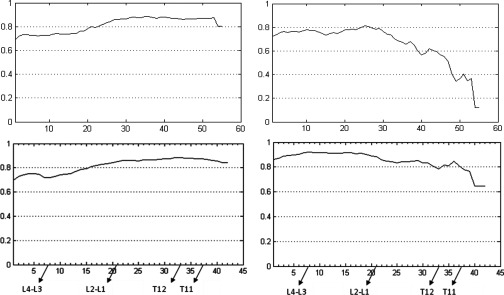
Correlation values from linear mapping (top row) and nonlinear mapping (bottom row) for SAT (left) and VAT (right). The vertical axis shows the correlation value. The horizontal axis shows the location of image slices (Slice 1 is at the inferior most position). Some key landmark positions are indicated along the horizontal axis in the bottom row.

Figure 7.

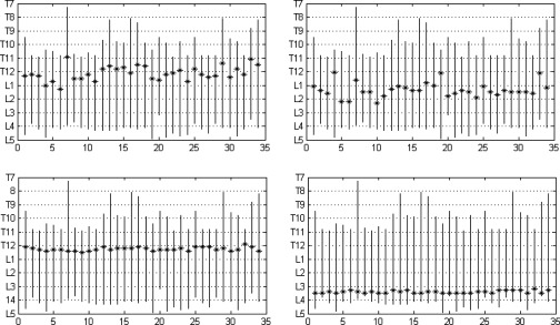
Anatomic locations (marked with “*”) of maximum correlation between (single) slice area and volume (SAT on left, VAT on right, linear method in top row, nonlinear method in bottom row). The horizontal axis shows subject numbers, and the vertical axis shows anatomic location from T7 to L5.

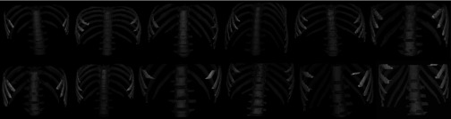
Figure 8.

Anatomic locations where maximum correlation is achieved for the two mapping methods. The top two rows are for SAT (left) and VAT (right) by using linear mapping; and the bottom two rows represent SAT and VAT for nonlinear mapping. The first and third rows are from the same subject, and the second and fourth rows are from another subject. The spine is used as a reference to show the slice locations (as a white line) of maximum correlation.

The following observations may be made from Figs. 6 to 8. The maximum correlation for VAT derived from nonlinear mapping achieved a 10% higher value than that of linear mapping. It is also clear that the maximum correlation occurs at different anatomic locations for SAT and VAT. With nonlinear mapping, the maximum correlation occurs at T12 for SAT and L3 for VAT as shown in the bottom figures in Fig. 6. The maximum correlation also occurs at different anatomic locations for the different mapping methods. For SAT and VAT, the locations of maximum correlation derived from linear mapping vary considerably among subjects. The goal of correlation calculation is to find one or more anatomic locations which are optimal for estimating abdominal fat distribution. The slices from all subjects used for correlation calculation are expected to be at the same anatomic location. Correlation testing will have no meaning if every subject has the slice considered for correlation calculation at a different location. The site of maximum correlation derived from nonlinear mapping has more precision than from simple linear mapping. In the bottom row of Fig. 7, there is a small variation of locations over all subjects which is less than 5.0 mm (same as slice spacing), implying that the slice localizations are anatomically very precise in the SAS (see Table 1). Table 2 shows the correlation derived from a single slice at different true anatomic locations where the maximum correlation for VAT occurs at L3-L4 and at T12-L1 for SAT. The results are similar to the correlation calculated from the nonlinear method as shown in the bottom row of Fig. 7. Again, the anatomic location of maximum correlation for SAT is different from that of VAT.

Table 1.

Correlation coefficients and slice location variation (in mm) for linear and nonlinear mapping techniques. Correlations shown are maximum values.

	Single slice at L4-L5		Linear mapping		Nonlinear mapping
	SAT	VAT	SAT	VAT	SAT	VAT
Correlation	0.74	0.87	0.89	0.81	0.88	0.92
Location variation (mm)	…	…	17.80	15.70	4.38	2.63

Table 2.

Correlation with single slice at different true anatomic locations.

	Correlation with single slice
Anatomic slice location	SAT	VAT
T10-T11	0.85	0.79
T11-T12	0.87	0.81
T12-L1	0.88	0.90
L1-L2	0.88	0.89
L2-L3	0.85	0.92
L3-L4	0.76	0.92
L4-L5	0.74	0.87

Examining the top two rows derived from linear mapping for SAT and VAT in Fig. 8, we observe that the anatomic locations of maximum correlation are significantly different for different subjects. Yet, for the nonlinear mapping, for both SAT and VAT, the anatomic locations of maximum correlation are much closer even though they come from different subjects. In particular, for the nonlinear mapping, there appears to be relatively constant high correlation values for SAT in the lower thoracic/upper abdominal region and for VAT in the lower abdomen.

To test the sensitivity of the results to the choice of the calibration data set, in Fig. 9 we show the single-slice correlation curves for SAT and VAT derived from a different set of randomly chosen five calibration data sets. The maximum correlation achieved was again 0.88 and 0.92 for SAT and VAT, respectively, which are the same as the results in Fig. 6, and the slice locations where fat volume maximally correlated with fat area are also the same. The curves are remarkably similar, as expected, except for some minor differences at the ends of the curves. Compared with linear mapping and earlier methods, one advantage of the proposed nonlinear mapping approach is to guarantee that the slice where maximum correlation occurs is at the same anatomical location irrespective of patient-to-patient anatomical variability.

Figure 9.

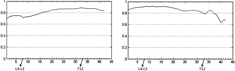
Correlation curves from nonlinear mapping derived from a calibration data set different from that used in Fig. 6. Left: SAT; Right: VAT. The vertical axis shows the correlation value. The horizontal axis shows the location of image slices (Slice 1 is at the inferior most position). Some key landmark positions are indicated along the horizontal axis.

Correlation with multiple slices

To address the question as to whether single slice or multiple (contiguous or noncontiguous) slices yield better area-to-volume correlation, we calculated the correlation by using multiple slices with both linear and nonlinear mappings.

Table 3 lists the maximum correlation achieved by using one, two, and three slices per subject with linear and nonlinear mapping. The correlation derived from the slice at the L4-L5 junction is also listed for comparison since this location is most commonly used. For this case, the choice of two and three slices is such that the slices are contiguous and they are as close to the L4-L5 junction as possible. Note that nonlinear mapping with multiple slices achieved the highest correlation. Table 4 lists anatomic locations where maximum correlation is achieved for the two methods. The locations of maximum correlation for SAT and VAT are again different, and the multiple slices achieving maximum correlation are not contiguous. For nonlinear mapping, the sites in the standardized anatomic space where maximum correlation is achieved are also listed in Table 4. One possible explanation for the findings is that discontinuous slice location combination may allow for a more representative sampling of the average fat area per slice across the abdominal region (vs the scenario where all the slices are from contiguous slices through the abdomen).

Table 3.

Correlation by using one or more slices per subject, where correlations shown are maximum values for the two mapping techniques.

Multiple slices		One slice	Two slices	Three slices
Linear mapping	SAT	0.89	0.90	0.91
	VAT	0.81	0.84	0.85
Nonlinear mapping	SAT	0.88	0.88	0.89
	VAT	0.92	0.95	0.95
Slices at L4-L5	SAT	0.74	0.74	0.75
	VAT	0.87	0.88	0.89

Table 4.

Slice locations after mapping (linear and nonlinear) where the maximum correlation is achieved. The values listed in the table are the slice numbers in the volume files (where number 1 indicates the bottom slice of the abdominal region and larger numbers are located closer to the top of the abdominal region). The anatomic locations in SAS are also listed for the nonlinear mapping.

		One slice	Two slices	Three slices
Linear mapping	SAT	36	27, 53	26, 52, 54
	VAT	25	4, 27	3, 25, 29
Nonlinear mapping	SAT	33 (T12)	22, 37 (L1-L2, T11)	22, 33, 35 (L1-L2, T12, T11-T12)
	VAT	8 (L3-L4)	8, 36 (L3-L4, T11)	8, 16, 36 (L3-L4, L1-L2, T11)

Figure 10 shows the correlation curves when multiple slices are used for correlation calculation. Here, only the results using two and three slices are shown since single slice results have been shown above. From Figs. 610, we observe that higher maximum correlation can be achieved when more slices are used for correlation calculation. The maximum correlation for VAT derived from nonlinear mapping is substantially (10%) greater than that from linear mapping as shown in Table 3. Especially note that the correlation curves for VAT go down considerably for certain combinations of two and three slices for linear mapping. This is due to the fact that the multiple slices are in fact from much different anatomic locations among subjects as in the single-slice case, while the nonlinear method performs much better since slices are selected anatomically more accurately in the standardized anatomic space.

Figure 10.

Correlation curves from linear and nonlinear mapping. Rows 1 and 2: SAT (left) and VAT (right) results for linear mapping using 2 and 3 slices. Rows 3 and 4 are similarly for nonlinear mapping. The vertical axis shows the correlation values and the horizontal axis shows the combination number for the different combinations among all possible choices of 2 and 3 slices. The oscillations seen are due to the systematic pattern of multiple slice number combinations.

CONCLUSIONS

Correlation analysis to determine the optimal anatomic slice locations in the abdomen for estimating body fat has not previously been performed to our knowledge. The optimal anatomic slice locations for single slice SAT and VAT estimation are not the same, contrary to common assumption. This result is important since these fat components may have different effects upon the pathophysiology of different disease processes. Use of multiple slices can achieve higher correlation than use of a single slice. The optimal locations of slices in this latter case are not contiguous. Experimental results on 50 abdominal CT image data sets showed that the standardized anatomic space created through nonlinear mapping of slice locations achieves better anatomic localization than linear mapping. The proposed method can be extended with greater or fewer landmarks than those adopted in this paper. We illustrated the method by using CT image data sets, and will continue to explore the applicability of this method on MR image data sets in the future. Overall, our conclusions are as follows:

1. The maximum area-to-volume correlation achieved is quite high, suggesting that it may be reasonable to estimate body fat by measuring the area of fat from a single anatomic slice at the site of maximum correlation. However, the site of maximum correlation and the degree of correlation itself may both depend on the particular patient group or disease condition studied. This paper focused on (near) normal male subjects in the age group of 50–60 years.

2. The site of maximum correlation is not at L4-L5 as commonly assumed, but is more superiorly located at T12-L1 for SAT and at L3-L4 for VAT. Furthermore, the optimal anatomic locations for SAT and VAT estimation are not the same, contrary to common assumption.

3. It is important to make sure that the slices for different subjects are selected at the same anatomic locations for correlation analysis. These locations seem to vary nonlinearly from subject to subject, at least for the population (G) and body region (B) considered in this paper. The proposed standardized space mapping achieves this consistency of anatomic localization by accurately managing nonlinearities in the relationships among landmarks. The dependence of VAT on the precision of anatomic localization seems to be far greater than that of SAT, perhaps due to the complex shape of the distribution of VAT compared to SAT.

4. Multiple slices achieve greater improvement in correlation for VAT than for SAT. The optimal locations of slices are not contiguous.

The goal of this research is to find optimal location(s) of slices for any given patient group and body region utilizing the data sets under any given image modality. Once the optimal locations are determined in the manner demonstrated in this paper, actual acquisition of images at precisely those locations in clinical practice can be implemented without much difficulty by making appropriate changes to the scan protocol, for example, by marking off plane locations on scout views.

One drawback of the proposed strategy is that it is difficult to implement on MR images since it is quite challenging to segment vertebral bodies in MR images. However, if certain features to tag anatomic locations reliably can be identified on slice images, then the method can be implemented in a straightforward manner.

References

- Flegal K. M., Carroll M. D., Ogden C. L., and Johnson C. L., “Prevalence and fends in obesity among US adults, 1999–2000,” JAMA 288, 1723–1727 (2002). 10.1001/jama.288.14.1723 [DOI] [PubMed] [Google Scholar]
- Joshi A. A., Ouchun H. Hu, Richard M. L., Michael I. G., and Krishna S. N., “Automatic intra-subject registration-based segmentation of abdominal fat from water–fat MRI,” JMRI 37, 423–430 (2013). 10.1002/jmri.23813 [DOI] [PMC free article] [PubMed] [Google Scholar]
- Choudhary A. K., Donnelly L. F., Racadio J. M., and Strife J. L., “Diseases associated with childhood obesity,” AJR, Am. J. Roentgenol. 188, 1118–1130 (2007). 10.2214/AJR.06.0651 [DOI] [PubMed] [Google Scholar]
- Arens R., Sin S., Nandalike K., Rieder R., Khan U. I., Freeman K., Wylie-Rosett J., Lipton M. L., Wootton D. M., McDough J. M., and Shifteh K., “Upper airway structure and body fat composition in obese children with obstructive sleep apnea syndrome,” Am. J. Respir. Crit. Care Med. 183, 782–787 (2011). 10.1164/rccm.201008-1249OC [DOI] [PMC free article] [PubMed] [Google Scholar]
- Vgontzas A. N., “Does obesity play a major role in the pathogenesis of sleep apnea and its associated manifestations via inflammation, visceral adiposity and insulin resistance?,” Arch Physiol. Biochem. 114, 211–223 (2008). 10.1080/13813450802364627 [DOI] [PubMed] [Google Scholar]
- Aziz H. P., Brett P. S., Jennifer L. R., Diego H., Catherine D. H., Pablo I., and Scott B. R., “Adipose tissue MRI for quantitative measurement of central obesity,” JMRI 37, 707–716 (2013). 10.1002/jmri.23846 [DOI] [PMC free article] [PubMed] [Google Scholar]
- Onat A., Avci G. S., Barlan M. M., Uyarel H., Uzunlar B., and Sansoy V., “Measures of abdominal obesity assessed for visceral adiposity and relation to coronary risk,” Int. J. Obese Relat. Metabol. Disorder 28, 1018–1025 (2004). 10.1038/sj.ijo.0802695 [DOI] [PubMed] [Google Scholar]
- Bandekar A. N., Naghavi M., and Kakadiaris I. A., “Automated pericardial fat quantification in CT data,” Proc. IEEE Eng. Med. Biol. Soc. 1, 932–935 (2006). 10.1109/IEMBS.2006.259259 [DOI] [PubMed] [Google Scholar]
- Positano V., Christiansen T., Santarelli M. F., Ringgaard S., Landini L., and Gastaldelli A., “Accurate segmentation of subcutaneous and intermuscular adipose tissue from MR images of the thigh,” J. Magn. Reson. Imaging 29(3), 677–684 (2009). 10.1002/jmri.21699 [DOI] [PubMed] [Google Scholar]
- Zhou A., Murillo H., and Peng Q., “Novel segmentation method for abdominal fat quantification by MR,” JMRI 34, 852–960 (2011). 10.1002/jmri.22673 [DOI] [PubMed] [Google Scholar]
- Engholm R., Dubinskiy A., Larsen R., Hanson L. G., and Christoffersen B. Ø., “An adipose segmentation and quantification scheme for the abdominal region in minipigs,” Proc. SPIE 6144, 1228–1238 (2006). 10.1117/12.652780 [DOI] [Google Scholar]
- Tong Y., Udupa J. K., Odhner D., Sin S., and Arens R., “Abdominal adiposity quantification at MRI via fuzzy model-based anatomy recognition,” Proc. SPIE 8672, 86721R1–86721R7 (2013). 10.1117/12.2007938 [DOI] [Google Scholar]
- Udupa J. K., Odhner D., Tong Y., Matsumoto M. M. S., Ciesielski K. C., Vaideeswaran P., Ciesielski V., Saboury B., Zhao L., Mohammadianrasanani S., and Torigian D. A., “Fuzzy model-based body-wide anatomy recognition in medical images,” Proc. SPIE 8671, 86712B (2013). 10.1117/12.2007983 [DOI] [Google Scholar]
- Maislin G., Ahmed M. M., Gooneratne N., Thorne-Fitzgerald M., Kim C., Teff K., Arnardottir E. S., Benediktsdottir B., Einarsdottir H., Juliusson S., Pack A. I., Gislason T., and Schwab R. J., “Single slice vs. volumetric MR assessment of visceral adipose tissue: Reliability and validity among the overweight and obese,” Obesity 20(10), 2124–2132 (2012). 10.1038/oby.2012.53 [DOI] [PMC free article] [PubMed] [Google Scholar]
- Ludwig U. and Klausmann F., “Whole-boy MRI-based fat quantification: A comparison to air displacement plethysmography,” Journal of Magnetic Resource Imaging 00: 00–00 (2014). 10.1002/jmri.24509 [DOI] [PubMed] [Google Scholar]
- So R., Matsuo T., Sasai H., Eto M., Tsujimoto T., Saotome K., and Tanaka K., “Best single-slice measurement site for estimating visceral adipose tissue volume after weight loss in obese, Japanese men,” Nutr. Metabol. 9, 56–65 (2012). 10.1186/1743-7075-9-56 [DOI] [PMC free article] [PubMed] [Google Scholar]
- Irlbeck T., Massaro J. M., Bamberg F., O’Donnel C. F., and Hoffmann U., “Association between single-slice measurements of visceral and abdominal subcutaneous adipose tissue with volumetric measurements: the Framingham heart study,” Int. J. Obese 34, 781–787 (2010). 10.1038/ijo.2009.279 [DOI] [PMC free article] [PubMed] [Google Scholar]
- So R., Sasai H., Matsuo T., Tsujimoto T., Eto M., Saotome K., and Tanaka K., “Multiple-slice magnetic resonance imaging can detect visceral adipose tissue reduction more accurately than single-slice imaging,” Eur. J. Clin. Nutr. 66, 1351–1355 (2012). 10.1038/ejcn.2012.147 [DOI] [PubMed] [Google Scholar]
- Sottier D., Petit J.-M., Guiu S., Hamza S., Benhamiche H., Hillon P., Cercueil J.-P., Krausé D., and Guiu B., “Quantification of the visceral and subcutaneous fat by computed tomography: Interobserver correlation of a single slice technique,” Diag. Interv. Imaging 94, 879–884 (2013) (available URL: http://www.sciencedirect.com/science/article/pii/S2211568413001393). 10.1016/j.diii.2013.04.006 [DOI] [PubMed] [Google Scholar]
- Machann J., Thamer C., Schnoedt B., Haap M., Haring H.-U., Claussen C. D., Stumvoll M., Fritsche A., and Schick F., “Standardized assessment of whole body adipose tissue topography by MRI,” J. Magn. Reson. Imaging 21(4), 455–462 (2005). 10.1002/jmri.20292 [DOI] [PubMed] [Google Scholar]
- Udupa J. K., Odhner D., Falcao A. X., Ciesielski K. C., Miranda P. A. V., Vaideeswaran P., Mishra S., Grevera G. J., Saboury B., and Torigian D. A., “Fuzzy object modeling,” Proc. SPIE 7964, 79640B (2011). 10.1117/12.878273 [DOI] [Google Scholar]
- Udupa J. K., Odhner D., Matsumoto M., Falcão A. X., Miranda P. A. V., Ciesielski K. C., Grevera G. J., Saboury B., and Torigian D. A., “Automatic anatomy recognition via fuzzy object models,” Proc. SPIE 8316, 831605 (2012). 10.1117/12.911580 [DOI] [Google Scholar]
- Nyul L. G. and Udupa J. K., “On standardizing the MR image intensity scale,” Magn. Reson. Med. 42, 1072–1081 (1999). [DOI] [PubMed] [Google Scholar]
- Grevera G., Udupa J., and Odhner D., “CAVASS: A framework for medical imaging applications,” Proc. SPIE 7497, 74971D1–74971D14 (2009). 10.1117/12.851180 [DOI] [Google Scholar]