Testing the optimality properties of a dual antibiotic treatment in a two-locus, two-allele model

Abstract

Mathematically speaking, it is self-evident that the optimal control of complex, dynamical systems with many interacting components cannot be achieved with ‘non-responsive’ control strategies that are constant through time. Although there are notable exceptions, this is usually how we design treatments with antimicrobial drugs when we give the same dose and the same antibiotic combination each day. Here, we use a frequency- and density-dependent pharmacogenetics mathematical model based on a standard, two-locus, two-allele representation of how bacteria resist antibiotics to probe the question of whether optimal antibiotic treatments might, in fact, be constant through time. The model describes the ecological and evolutionary dynamics of different sub-populations of the bacterium Escherichia coli that compete for a single limiting resource in a two-drug environment. We use in vitro evolutionary experiments to calibrate and test the model and show that antibiotic environments can support dynamically changing and heterogeneous population structures. We then demonstrate, theoretically and empirically, that the best treatment strategies should adapt through time and constant strategies are not optimal.

1. Introduction

The discovery of antibiotics provided medics with a tool of unprecedented potency in the battle against bacterial pathogens [1]. However, we are now engaged in an arms race where bacteria seem to be, at least for the moment, firmly in the ascendancy and new ideas for deploying antibiotics are needed. Bacteria have evolved resistance to every antibiotic in clinical use [2], and the correlation between drug usage and resistance evolution [3] suggests our attitudes towards antimicrobials are, at least in part, responsible for our problems. Antibiotics have been misused [4] and overprescribed [5], and problems in the economic model due to resistance have lead the pharmaceutical industry to abandon their antimicrobial discovery programmes [6,7].

However, simply finding more antibiotic small molecules will not provide a sustainable solution to these issues. The timeline from antibiotic discovery to drug-resistant clinical isolate is of the order of a decade, or two [3], so unless we have a library of drug usage protocols successful both at clearing bacterial infections and at preserving their efficacy, any novel antimicrobial substance would be predestined to eventual failure.

Finding long-lasting solutions to antibiotic resistance is an exceptionally difficult problem, well-beyond the scope of a theoretical study such as this, but we contend that theoretical frameworks exploiting the theory of dynamical systems, control and optimization might be developed that provide insight and contribute much to the design of rational drug deployment strategies.

With this in mind, we ask the question: what if treatment fails to achieve inhibitory doses everywhere at all times and resistance develops? What principles might there then be behind optimal dosing strategies? Seeking answers, we pose a pharmacogenetics theoretical model of an experimental microcosm (with parameter values calibrated using in vitro experimental data) and use it to illustrate a very simple control engineering principle: the optimal treatment is contingent upon treatment duration and, as a result, the treatment may need to be adapted through time.

1.1. Optimal antibiotic treatments

An optimal antibiotic deployment strategy is often seen as having two features to reconcile: (i) the dose and (ii) the duration of treatment, both are a matter of some controversy.

First, there is no consensus on the optimal length of treatment. It has been reported that the number of pills per patient favours odd over even numbers, the reason behind this statistical anomaly is an unwritten rule, whereby treatment duration has to be ‘5 or 7 days, or multiples thereof’ [8]. There is no agreement on the precise length of treatment but medical textbooks emphasize that therapies should favour treatments of longer duration and that the premature interruption of treatment promotes the evolution of drug resistance [9]. This stems from the idea that overdosing with antibiotics is, at worse, therapeutically neutral and no harm results from taking drugs for prolonged periods. However, mounting clinical [10], experimental [11] and theoretical [12] evidence suggests that short-course therapy can be as effective without imposing selective pressures that favour resistant mutants. These issues have been debated openly in the literature with ensuing disagreement between different communities [13–15]. More recently, the study of Martinez et al. [11] is clear in emphasizing treatments ‘as brief as clinically appropriate’.

With respect to the optimal dose, current practice indicates that high doses of antibiotics are more effective at suppressing drug-resistant bacteria (discussed in [16]). One argument states that by minimizing population size, we also minimize the probability of occurrence of a de novo genetic mutation conferring drug resistance upon bacteria. This is the ‘hit early, hit hard’ strategy documented as early as 1913, several years before the discovery of penicillin [17].

But high drug concentrations are known to produce side-effects and doses cannot be indiscriminately increased [18]. Not only are high antibiotic dosages toxic [9,19], they can disrupt the ecological stability of the commensal microbiota, allowing pathogens to colonize the host [20]. A strategy for increasing drug potency while decreasing drug concentration is the use of multidrug cocktails [21]. Synergistic antibiotics, whereby the combined effect of two drugs is greater than expected given the efficiency of either on their own, have been actively sought for decades [22].

Some have questioned whether aggressive chemotherapies are an appropriate strategy to prevent resistance [23,24]. These studies have shown that if the initial phase of treatment is unsuccessful at clearing the pathogen, then surviving drug-resistant genotypes may thrive in an environment in which many of the drug-susceptible competitors have been eliminated. It has also been shown that synergistic combinations can accelerate the evolution of antibiotic resistance [25] and, as a result, it was suggested that ‘antagonistic’ drug interactions, seemingly neglected in clinical practice, might slow resistance evolution [26]. In practise, drugs are used even when their synergy is not proved, for example the anti-MRSA combination vancomycin and rifampicin [27,28].

2. A mathematical abstraction

Seeking to understand how mathematics can address questions in antibiotic optimality, we begin with an abstract framework applicable to many mathematical models. From the mathematician's perspective, what we are about to say is self-evident: the optimal control of an adaptive system is unlikely to be realized with control strategies that are constant through time.

To demonstrate more precisely what we mean by this, consider a smooth dynamical law, f, subject to controls, u and v, so that the mathematical model class we analyse has the following form:

2.1

where is a state variable, u(t), are controls and T > 0 is a fixed terminal time for antibiotic treatment; u and v represent the dosages of two different antibiotics whose optimal combination we wish to find. Thus, given fixed dosages u₀ > 0 and v₀ > 0, we let θ ∈ [0, 1] denote the relative drug dose, we define an objective functional, J, by

2.2

where is a weight vector. Here, and throughout, denotes Euclidean inner product.

For each u₀, v₀ and T > 0, under mild restrictions on f, like smoothness, there is an θ_opt(T) that satisfies

2.3

where the minimum here is taken over a compact subset of the reals: finding the optimal relative drug dose here is a finite-dimensional optimization problem and the existence of a minimizing value of θ is therefore guaranteed.

For u and v to represent antibiotic drugs, we should also assume the following properties:

whenever u ≥ 0 and v ≥ 0. In other words, increasing the dose of both drugs will reduce the growth of the microbial population in the components of the weight vector, w.

Definition 2.1 (synergy). —

Define the ‘interaction function’

and suppose the basal drug concentrations, u₀ and v₀, are calibrated to have equal inhibitory effect: i(0) = i(1). Strict drug synergy is said to hold in (1) when i is convex: i″(θ) > 0 for all θ ∈ (0, 1). We define the most synergistic combination, θ_syn ∈ (0, 1), to be the value of θ for which the minimum of i(θ) occurs.

For completeness, we also include the following definition.

Definition 2.2 —

(antagonism). Suppose that the basal drug concentrations u₀ and v₀ are calibrated to equal inhibitory effect: i(0) = i(1). Strict drug antagonism is said to hold in (1) when the function i(θ) is concave: i″(θ) < 0 for all θ ∈ (0, 1).

Figure 1 illustrates synergy and antagonism that relates these two theoretical definitions to how synergy and antagonism are seen in empirical datasets known as ‘checkerboards’. In practise, the weight w would be chosen so that i(θ) represents the dependence of total population density on the relative drug proportion, θ.

Figure 1.

The drug interaction profile, i(θ), is related to empirical ‘checkerboards’ that are illustrated in (a,c). In the latter, the concentration of both drugs (called ‘D’ and ‘E’) is given on the x- and y-axes, bacterial growth inhibition (or population density or some other fitness measure) is then plotted on the z-axis. The contour of all concentrations that reduce this measure by half is an isobole here denoted IC⁵⁰, and figures (a,c) show two checkerboard plots viewed from above. Basal concentrations of both drugs that achieve the same inhibitory effect in this illustration are D⁵⁰ and E⁵⁰, θ then parametrizes the equidosage line between these two values. The fitness measure evaluated along this line is shown in (b,d) and we define the degree of interaction based on this curve, this is i(θ). We say the interaction is synergistic when the drug proportion that minimizes i(θ) satisfies 0 < θ < 1 as in (b), we denote the resulting value by θ_syn. In (d), we observe θ_syn=0 or θ_syn=1, in this case the drugs are said to be antagonistic as i(θ) is maximized by a drug combination. Adapted from [24]. (Online version in colour.)

Suppose that the two drugs in (2.1) are synergistic and proceed by Taylor expanding the functional J with respect to T. If we write solutions of (2.1) as x = x(t;θ, T), then

where and we find

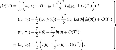2.4

where We now define so that the minima of J and j therefore coincide.

From the strict drug synergy property, the minimum of j(θ, 0) occurs when θ = θ_syn ∈ (0, 1). Moreover, at the minimum of j, there results provided T is small enough. As which is a non-zero quantity by the assumption of strict drug synergy, we may solve for θ as a function of T by applying the implicit function theorem. At this solution, θ = θ_opt(T), say, and it follows by definition that θ_opt(0) = θ_syn. Hence, because ,

and, differentiating with respect to T, we establish

On setting T = 0, it follows that

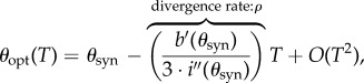because

In other words, when we compare with the strategy of optimal drug synergy with the optimal combination, with respect to a wide range of possible measures, provided the genericity condition is satisfied, these two concepts are only close for a period of time that depends explicitly upon the reciprocal of the strength of synergy of the drug.

2.1. Comments

There are many optimality criteria we could have chosen in (2.3). If we were to let T > 0 be free and then define

noting that x now depends on T explicitly, one could determine an optimal control (u*, v*, T*) for which

This has a larger space of admissible controls than (2.3) and it also includes the terminal time T as an unknown. One could argue that this new functional represents the essential property of what we desire in an optimal antibiotic combination treatment: it determines both the optimal dosages and the terminal time at which to stop treatment.

However, the purpose of continuing to use J as the objective functional here is to yield a set of theoretical predictions that can be tested empirically by reducing the optimal combination question to a one-dimensional problem on the ‘equidosage line’. The latter is a line in the two-drug plane of concentrations that is determined by the dosages , where 0 ≤ θ ≤ 1.

3. An evolutionary experiment

Antibiotic dose–response profiles are usually determined using disc diffusion susceptibility testing [29] or by taking fixed-time (a.k.a endpoint) density measurements in liquid media [30]. Here, we employ the latter because we can use shaken microtitre plate readers to quantify the dynamics of bacterial population densities through time and, based on observed growth kinetics, thereafter determine drug susceptibility at different antibiotic dosages.

In the following, we use a standard batch-transfer experimental protocol (see appendix A) to treat bacteria. This is often used to study adaptation to antibiotic environments [24,25], whereby a shaken environment with liquid growth medium is inoculated with bacteria that are cultured in an array of wells for a fixed period of time. Population densities are measured continually for 24 h at which time a fixed volume is sampled from the flask and transferred to a new well containing fresh growth medium and antibiotics. The repetition of this process defines the batch-transfer protocol.

In the remainder, we have two antibiotics at concentrations denoted by D(t) and E(t) at time t. We use B(t) = (B⁽¹⁾(t), …, B⁽ⁿ⁾(t)) for the vector containing the density of n bacterial phenotypes differing in their dose–response profiles and S(t) will denote the concentration of an essential but limiting carbon source supplied to the bacteria.

Each experiment consists of N transfers. If each transfer has a duration of T hours, with t ∈ [0, T], the state of the system at any time is

where a subscript has been placed on B to denote the phenotypic densities each day and so i = {1, 2, …, N + 1}. The initial density of bacteria after transfer i is a small proportion of the terminal state of the previous day and, as illustrated in figure 2, if denotes this proportion then the initial condition of transfer i > 1 will satisfy

where 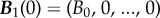is the density vector of the bacteria on the first day. In practise, B₀ will represent around 10⁵ cells per millilitre in any one of our experimental protocols that are described later.

Figure 2.

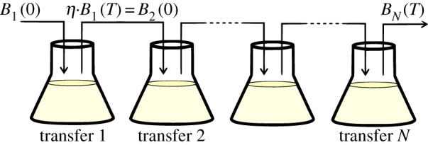
Schematic illustration of a batch-transfer experiment. A small population of bacteria is inoculated and cultured under essential resource limitation for N units of time. Then, a fraction η of the population is transferred to a new flask containing fresh medium and antibiotics and the process is repeated for several days. (Online version in colour.)

The population dynamics of the bacteria competing in this environment can be written as a single differential equation

3.1a

where F is a model-specific mapping described in §3.3 and the initial condition

3.1b

applies each day where Here, S₀ is a fixed parameter denoting the initial concentration of the limiting resource each day, D₀ and E₀ are also fixed and represent the basal concentrations of antibiotic supplied.

3.1. Modelling the action of bacteriostatic antibiotics

The bacteriostatic antibiotics we use suppress the bacterial growth rate by inhibiting protein synthesis and we represent the action of the drug by viewing it as a suppressor of biomass synthesis. So, suppose each cell ingests the essential resource from the environment as a process following Monod kinetics:

3.2

where V_max represents the maximal resource uptake rate and K is a half-saturation constant.

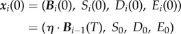
The growth rate of each bacterium depends on the concentration of antibiotic present in the environment, so we assume the above uptake function is modulated by an antibiotic-dependent coefficient c(D) that converts units of the limiting resource to biomass and describes the efficiency of cell production per unit resource in the presence of antibiotic. Thus, the per-cell, per-unit time growth rate can be written as We will write c(D) as a product of the cell conversion rate in a drug-free environment, c, and a dimensionless inhibition coefficient that depends on the concentration of antibiotics

3.3

Forms for γ(D) can be derived using standard enzymatics [31] and if we suppose that the antibiotic suppresses growth due to a competitive inhibition process, then the following expression is consistent [31] with antibiotic-target binding data for rifampicin-like drugs:

3.4

where κ₁ and κ₂ are parameters characterizing susceptibility to the antibiotic.

3.2. Multidrug interactions in a model cell

To extend the rationale of §3.1, assume two antibiotics are present in the environment at concentrations D and E. Again, bacterial growth is modelled as a Monod term multiplied by a growth inhibition coefficient, γ(D, E), so G(S, D, E) = c u(S)γ(D, E), where c is a conversion rate and u(S) is the resource uptake function defined in equation (3.2).

Now, γ(D, E) is a function, whereby γ(D, 0) = γ_D(D) and γ(0, E) = γ_E(E), and γ_D(D) and γ_E(E) are inhibition functions describing the action of each antibiotic deployed alone.

The shape of the contours of γ(D, E) determines the antibiotic interaction [32]. In particular, we use two bacteriostatic antibiotics of different functional classes with a known synergistic interaction [24,25]: erythromycin (E), a macrolide that binds to the 50S ribosomal RNA subunit and doxycycline (D), a tetracycline that binds to the 30S ribosomal RNA subunit. As these drugs have non-overlapping targets, we model their interaction as non-exclusive competitive inhibitors [33] and the growth inhibition coefficient for a multidrug combination of D and E is

3.5

where κ_d, κ_e and κ_m are positive constants. Note that κ_m controls the strength of synergy and if it is zero, the drug interaction is additive.

Assuming cell yield (defined as the maximal cells produced per essential resource) is the same for four genotypes (drug-susceptible wild-type, D-resistant, E-resistant and DE-resistant), the growth rate and antibiotic susceptibility patterns for different bacterial strains will be characterized in terms of a vector of parameters, 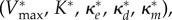where the asterisk is a placeholder for the genotype under consideration. For instance, we will denote an antibiotic-susceptible bacterial wild-type with the superscript s and its growth rate will be written as

By contrast, a multidrug-resistant mutant (represented by a superscript m) would have, by definition, a higher growth rate than susceptible bacteria at high concentrations of antibiotics. Thus, if the growth rate of a multidrug-resistant mutant is given by the function

then, to represent greater resistance, there must exist a critical drug combination (D*, E*) for which

Antibiotic resistant cells often encounter a reduction in fitness in an antibiotic-free environment, a so-called fitness cost of resistance [34]. In our framework, this can be realized by imposing a lower resource uptake rate and, therefore, a lower growth rate in an antibiotic-free environment

As an illustration, figure 3 contains the contour plots of growth functions, G^*(S, D, E), at fixed resource concentrations but at different drug doses for susceptible, single-drug-resistant and multidrug-resistant bacterial genotypes; there are four such functions G^s, G^d, G^e and G^m, one for each genotype. Note how the contour lines are concave in all four cases and, therefore, the drug interaction is synergistic for each genotype.

Figure 3.

Contour plots of the drug inhibition surface γ(D, E) for different bacterial phenotypes (parameter values contained in table 1). Each line represents a 10% decrease of growth rate at a fixed concentration of resource (S₀ = 2000 μg ml⁻¹). (a) Susceptible phenotype, (b) E-resistant, (c) D-resistant and (d) multidrug, DE-resistant bacteria. (Online version in colour.)

3.3. Resistance mutations

Susceptible bacteria can acquire resistance through the horizontal transfer of mobile genetic elements [35], through single point mutations in drug targets [36] or through the amplification of genomic regions containing resistance genes [37]. Seeking to understand how target modification affects the optimality properties of antibiotic combinations, we model resistance adaptation by allelic changes in two independent genetic loci.

Susceptible genotypes evolve resistance due to point mutations occurring at rate ε > 0 (per cell per division) in an ‘E-resistance’ locus and a ‘D-resistance’ locus. The accumulation of two mutations confers multidrug resistance. The mutation structure on these loci can be described by a mutational matrix

Here, I is the identity matrix, ε the rate of mutation and M is a stochastic matrix whose entries, m_ij, control the rate at which bacterial type j mutates into bacterial type i.

If 1 denotes a vector of ones of the appropriate dimension, then the mutational matrix is stochastic

We assume M (and therefore ) is irreducible in the sense that for each pair (i,j), there is a number p = p(i, j) such that the (i,j)th entry of M^p is non-zero.

Our model will be completed when we describe the mapping, F, in (3.1a) that defines the ecological setting for the above genetics. We are modelling the densities of four different genotypes: a susceptible wild-type at density are resistant mutants to drugs D and E, respectively, and is the multidrug-resistant mutant. We then define a vector that contains the densities of each strain,

and the dynamics (at transfer i) of this two-allele, two-locus model can be written as

3.6a

3.6b

3.6c

and

3.6d

Here, G(S, D, E) is the vector (G^s, G^d, G^e, G^m) and the dot in (3.6a) denote pointwise multiplication. The parameters d and e are binding constants of each antibiotic to each bacterial genotype and the parentheses in (3.6b) denote the standard Euclidean inner product.

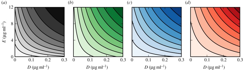
Figure 4 illustrates a simulation of equation (3.1), as defined by equation (3.6), where the transfer occurs every 12 h and an ED-combination treatment has been used. As the number of transfers increases, the multidrug-resistant ED-genotype (shown in red) outcompetes the other genotypes and we see expected behaviour in that this genotype sweeps through the population as it adapts to the presence of both drugs. For comparison, figure 4b shows experimental data obtained for Escherichia coli adapting to a multidrug environment that contains 7 μg ml⁻¹ erythromycin and 0.3 μg ml⁻¹ of doxycycline where total population density is shown for each transfer.

Figure 4.

Adaptation to multidrug environments in a batch transfer experiment. Escherichia coli is cultured for 12 h before propagating a fraction of the terminal population into the next season (a.k.a transfer) containing fresh growth medium and both antibiotics. (top) A simulation of the model defined by (3.1) and (3.6) using parameter values in table 1. The four different shaded areas represent densities of each of the bacterial genotypes (where there is one for drug-susceptible, then E-resistant, D-resistant and multidrug-resistant mutants). (bottom) Optical densities obtained experimentally (E. coli AG100 cultured in 7 µg ml⁻¹ erythromycin and 0.3 µg ml⁻¹ of doxycycline), the areas shown show the mean growth dynamics of eight replicates whereas the lines denote standard errors at each time point. (Online version in colour.)

4. Preliminary results

4.1. Population heterogeneities and non-monotonic dose–response

Antimicrobial susceptibility tests can be difficult to standardize [38], but they are widely used to determine important quantitative pharmacodynamic parameters characterizing the inhibitory relationship between antibiotic and bacteria [39]. For bacteriostatic antibiotics, a dose–response curve that showing densities at a given timepoint at a series of increasing dosages characterizes the effect of the drug. An important feature of this is the so-called minimum inhibitory concentration. This is the lowest drug dosage at which a 99.9% reduction in bacterial density can be achieved at that timepoint by the use of the drug. By the very nature of antibiotics, we expect dose–response data to be monotonic decreasing.

We therefore evaluated the effect of resistance adaptation on the dose–response curve with the following experiment. A clonal population of E. coli bacteria (several different strains were used) was inoculated into a 96-well microtitre plate containing different concentrations of a single bacteriostatic antibiotic, in this case erythromycin, at a concentration E measured in μg ml⁻¹. After 24 h, following the batch-transfer protocol, we transferred a small volume from each well into an identical plate but with fresh growth medium and antibiotics. We repeated this procedure for 5 days (see appendix A for more detailed experimental methods).

Figure 5b illustrates the population densities at the end of each day in this protocol (density here is the optical density of the population measured at a 600 nm wavelength).

Figure 5.

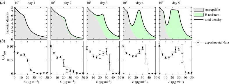
Non-monotonic dose–response curves in serial-transfer experiments. Row (a) illustrates simulations of a model based on (3.6) (using parameters in table 1), whereas row (b) illustrates optical densities of E. coli (strain AG100) measured at 24 h intervals at different concentrations of the drug erythromycin (E). Each column shows a dose–response curve for each day. Note how the characteristic, monotone dose–response curve of day one becomes a non-monotone curve due to a sub-population of resistant phenotypes that emerge more quickly at higher doses (error bars here and throughout denote standard error, eight replicates). (Online version in colour.)

The first day's dose–response curve has the common characteristic to these datasets: first a plateau, then a sharp drop as the dose increases. By the second day, there appears to be a small protuberance at intermediate drug concentrations. As the experiment proceeds, this protuberance is more pronounced, eventually producing a non-monotonic dose–response curve. This phenomenon is related to the Eagle effect that was first described in 1948 where non-monotonic dose–response relationships were noted at low cell densities [40].

Equations (3.6a–d) provide a mechanistic explanation of the observed non-monotonicity in the dose–response curve. Simulations of the model (implemented without doxycycline, so that ) shown in figure 5a illustrate how intermediate drug concentrations support coexistence between the susceptible strain (the grey area) and the E-resistant strain (the green area; E for erythromycin). By contrast, the fitness cost paid by the resistant cells at low antibiotic concentrations is large enough that this environment selects the susceptible bacteria, while at high drug doses only the resistant phenotype is able to persist. While this is not the same observation as that made by originally by Eagle in 1948, it might be appropriate to call this phenomenon an ‘adaptive Eagle effect’ as it only appears after the initial population has adapted to the presence of the drug.

It is noteworthy that this unusual behaviour of an adaptive dose–response profile can be captured by such simple genetical and ecological assumptions, this gives us some confidence that the model is able to capture features that might not be evident from verbal reasoning alone.

4.2. Multidrug interactions are dynamic

The standard test used to determine the degree of interaction of a pair of antibiotics is a two-dimensional dose–response surface known as a checkerboard [41]. The horizontal axes are the dosages of the drugs and the vertical, z-axis represents the density of the bacterial population measured experimentally at some time. Based on the shape of the lines of equal inhibitory effect in the checkerboard that are known as isoboles, one characterizes the interaction between the two drugs as follows [22]: if the isoboles are convex the interaction is synergistic, if they are concave the drugs are antagonistic.

We performed a checkerboard experiment (using 256 different drug combinations with 11 replicates, see appendix A) using erythromycin (E) and doxycycline (D), drugs with an established synergy [25]. As expected, the isoboles exhibited the characteristic of a synergistic interaction as can be seen in the bottom-left panel of figure 6a). We then took samples of bacteria from this experiment containing a highly synergistic combination (E₀ = 4.8 μg ml⁻¹, D₀ = 0.08 μg ml⁻¹) and used these to inoculate a new batch-transfer experiment. After four daily transfers, we used the resulting evolved bacterial populations to determine another checkerboard, the purpose of which was to determine how the adaptation to a synergistic environment would be manifested within the isoboles of the dose–response surface.

Figure 6.

Empirical and theoretical checkerboards. (a) A dose–response surface, or isobologram, of E. coli MG4100 grown in a glucose-limited environment under the effect of different concentrations of doxycyline (D) and erythromycin (E) when measured on days 1 and 5 (11 replicates). (b) Numerical simulations of the two-locus, two-allele model (parameters in table 2) illustrates the dynamic nature of the population structure. Boxes (c) show bacterial genotypes with the highest frequency with colour intensity proportional to the density of each type. By day 5, the multidrug-resistant genotype (‘DE-resistant’) has the highest density at high drug concentrations, at low concentrations the susceptible has the highest densities and the single-drug-resistant phenotypes (E-resistant and D-resistant) are over-represented near each axis. (Data first appeared in [24], the analysis and interpretation is new.) (Online version in colour.)

Figure 6 shows that the checkerboard has shifted in the sense that higher densities are produced at higher drug concentrations, consistent with drug-resistance adaptation. However, the data in figure 6 are too coarse to allow a conclusive analysis on whether the synergy that was present on day 1 still remains 4 days later. It is probably unwise to scrutinize the subtleties of this surface too closely in terms of how it relates to the nature of the drug interactions, the data being as sparse as it is. In order to address our question, we use a different analysis technique that gives more precise information on the drugs' interaction.

4.3. A two-locus, two-allele smile–frown transition

Our definition of synergy and antagonism is stated in terms of two possible instances of the function i(θ) in definitions 2.1 and 2.2. In these definitions, a convex form for i(θ) corresponds to synergy, a concave i(θ) corresponds to antagonism. However, a phenomenon can arise, whereby synergism is lost and in [24] this was termed the ‘smile–frown transition’.

In this transition, a short-term synergy is replaced by an antagonism in the data because the most potent combinations select most for drug-resistant genotypes. As a result, population density data are ‘inverted’ and the characteristic, convex U-shape of synergy gives way to a near-concave W-shaped pattern that represents an antagonism. The population density data in figure 7a,b, respectively, show this transition both in data and in an instance of the population genetics model presented above.

Figure 7.

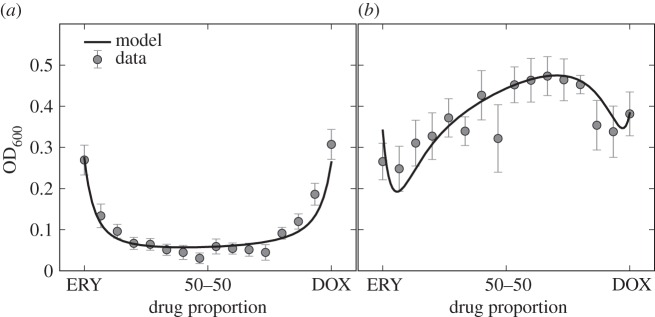
The smile–frown transition in optical density data. Both figures show optical density of E. coli MG4100 as a function of the variable θ, the relative drug concentration: θ = 1 corresponds to DOX and θ = 0 corresponds to ERY. The left-hand figures shows, after 12 h (a) growth, that these two drug act synergistically on the population, whereas the 36 h (b) data shows an antagonistic profile. At 12 h, population density is minimized by a drug combination because of the synergy, whereas at 36 h the same combination maximizes population densities. (This dataset appeared in [24], the model fit to that data is new.)

The relevance of this observation, made of population-level data, can be understood in the context of the ‘search for synergy’ [22] if we re-visit the growth functions, G^*(S, D, E), used in equation (3.6). According to that model, the function 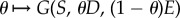is convex (i.e. synergistic) for all S, D and E (figure 3) and yet the population-level outcome that results from simulating this model need not respect that synergy because of a population structure that arises during treatment (figures 6 and 7). One could interpret this by stating that single-cell synergy does not imply an ‘evolutionarily robust population synergy’.

Informally, the changing drug interaction pattern in figure 7 could be seen as two conjoined copies of the data from figure 5 in the sense that the smile–frown transition is due to two emerging, non-monotone dose–response profiles laid contiguously, side by side.

4.4. The optimal drug combinations can depend upon treatment duration

The subtle, frequency- and density-dependent effects that produce non-monotone dose–responses and the smile–frown transition suggest that what dose and combinations are optimal for a treatment that lasts 1 day might be different from a treatment that lasts longer.

To address this, we need to define what we mean by an optimal treatment: an optimal drug combination needs an objective. In our context, we could use a criterion that measures the inhibitory effect of an antibiotic using, perhaps, only on the total density of bacteria found at the end of the experiment. Or else, we could measure the totality of bacterial cells produced by each treatment. These measures, however, only account for bacterial yield and could therefore completely fail to capture the reduction of growth rate induced by a bacteriostatic antibiotic.

Indeed, two experiments can have similar final bacterial densities but with very different growth dynamics to achieve those densities.

To overcome this, we use an optimality measure of treatment success that incorporates the total observed bacterial density in an experiment of N days in an objective functional and we will refer to this as the cumulative area under the curve (AUC), , defined as follows:

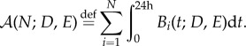4.1

Experimentally, this quantity can be approximated by measuring bacterial density continually and then applying a numerical integration rule over the empirically determined daily growth curves. In our experiments, this is done every 20 min thus producing a timeseries of population densities each day, labelled i, that depends on the drugs used, (D, E). The population density timeseries is therefore written as B_i(t; D, E).

We normalize this measure with respect to a drug-free control population and so compute AUC inhibition, a dimensionless performance index we refer to in the remainder as

4.2

This objective functional takes values in the interval [0,1] and if the antibiotics have completely inhibited bacterial growth, if the drugs have no effect.

To make a comparison between the efficacy of different drug cocktails a fair one, we perform the following calibration. We determine ‘basal’ concentrations of erythromycin and doxycycline from their single-drug dose–response curves so that each drugs' monotherapy achieves equal inhibitory effect on growth at 24 h. So, if we denote by E₀ and D₀, those basal concentrations, respectively, we then represent fixed-dose combinations of the two drugs by a dimensionless drug proportion coefficient, θ. Each drug combination used to treat bacteria experimentally therefore lies on the equidosage line (θD₀, (1 − θ)E₀), where 0 ≤ θ ≤ 1.

The drug proportion θ remains constant throughout the experiment and, therefore, any bacterial population is initially exposed to the same, fixed-dose multidrug concentrations throughout the treatment. This assumption, however, does not imply that the environmental drug concentration remains constant at all times because concentrations decrease as drug molecules enter the cell and bind to their targets. Antibiotic molecules also degrade naturally over time in solution.

We now take θ to be our control variable and define the optimal drug proportion to be the combination that maximizes the objective functional in (4.2), a quantity we denote θ*. The optimal drug proportion is now determined by solving the following one-dimensional optimization problem:

4.3

Now, by definition of synergy, the short-term, N = 1, optimal drug combination for this synergistic drug pair must correspond to the combination that maximizes the synergistic effect. Thus, a near 50–50 combination treatment should be optimal when N = 1, this would be represented by the optimal control residing at, or close to θ^* = 1/2.

However, does this synergistic value for the optimum remain so for a longer term experiment, when N > 1? We expect that for each N ≥ 1, there is an associated optimal value, θ^*(N) and by virtue of the synergy θ^*(1) ≈ 1/2. We now address the behaviour of this function as measured experimentally using a batch-transfer protocol as N grows.

Figure 8 is a representation of an empirical and a theoretical dataset, giving a comparison of the optimal combination obtained experimentally (figure 8b) with the optimal combination computed using the two-locus, two-allele model defined by equations (3.6a–d) (figure 8a). As expected from the synergy, in both cases the optimal 1-day drug proportion corresponds to the drug combination that maximizes synergy, but the optimal drug proportion changes when we treat for longer durations. For example, if we wanted a treatment lasting 5 days, it is then preferable according to our measure of success to deploy a single drug instead of a two-drug cocktail.

Figure 8.

The optimal drug combination depends on the length of the experiment. The optimal drug combination as a function of the length of the experiment: the colour gradient represents the normalized cumulative AUC inhibition (white represents maximum inhibition, and black the minimum inhibition) of E. coli MG4100. The dotted line corresponds to the optimal drug proportions as a function of the length of the experiment. (a) Simulations of the theoretical, two-locus, two-allele model from (3.6) using parameters in table 2. (b) Empirical data: each circle represents a different drug proportion tested experimentally. Note how, both in the experiment and the model, at the beginning of the experiment the optimal treatment corresponds to the combination treatment that maximizes synergy, but for longer treatments the model and the data coincide in the sense that the optimal strategy uses more and more erythromycin. In an experiment of 5 days, it would have been better not to combine the drugs at all, at least according to this optimality measure. (Online version in colour.)

5. Conclusion

We have shown that an optimal drug combination can depend on the duration of the treatment (the parameter N above). So, for each treatment of length N, there is control strategy (a.k.a. relative drug combination) θ^*(N) that is optimal, moreover θ^*(N) is not a constant function of N. This result is not surprising from a theoretical control perspective as complex, adaptive systems are unlikely to be controlled optimally using constant, non-responsive controls. Note that we have not determined the optimal treatment, we have only demonstrated that the optimal combination along the equidosage line depends on the length of treatment.

Although this is a laboratory study data analysed using a model inspired by drug target modification, there are other ways in which bacteria resist antibiotics. Resistance to erythromycin and doxycycline is also conferred by the product of an operon acrRAB and the gene tolC that form an efflux pump spanning the inner membrane, periplasm and outer-membrane in E. coli. Treating with these drugs is known to lead to genomic duplication events where around 8% of the E. coli genome is duplicated in which acrRAB is sited [24]. A contribution of this study is to show that the smile–frown transition of the previous study [24] can be realized theoretically by target modification, not only by pump duplications.

Nevertheless, although we have not tested the idea directly, our data indicate that actively changing the antibiotics used during treatment, or changing the way they are combined, may be one path to explore further at higher dosages. Mycobacterium tuberculosis is, in some sense, treated in this way [42] but it might also be possible that other pathogens could be treated successfully with regimens that change through time, but such sequential regimens are not common. There is clinical evidence to show that sequential treatments of Helicobacter pylori can outperform combination treatments at the same dose [43,44], although not all trials have been equally successful [45].

Clinicians are well in advance of our theory, having trialled a range of strategies to combat resistance evolution. The recent development of personalized, rapid-diagnosis devices to determine the pathogen responsible for infection with patient-specific, DNA-based testing so the most appropriate drug can be given as soon as possible [46,47] is one such advance. For a review of the many protocols trialled in practice, see [48]. However, there could be a role for data-driven optimal control theory that can highlight new strategies in the search for treatments that help combat resistance.

Data accessibility

Data can be downloaded directly from http://people.exeter.ac.uk/reb217/data.html or by sending a request by email to the corresponding author.

Appendix A. Experimental methods

Escherichia coli K12 (strains AG100 and MC4100) were used throughout and cell inoculations were taken from the same colony of each strain for all the experiments conducted. Experimental populations were cultured in M9 medium at 30°C with the following concentrations: part A: 350 g l⁻¹ K₂HPO₄, 100 g l⁻¹ KH₂HPO₄; part B: 29.4 g l⁻¹ trisodium citrate, 50 g l⁻¹(NH₄)₂SO₄, 5 g l⁻¹MgSO4. Parts A and B were 50× stock solutions in deionized water, sterilized by autoclaving. For M9 minimal medium, they were diluted in water accordingly with 0.2% glucose and 0.1% casamino acid added as nutrients.

The antibiotics used are erythromycin and doxycycline (both Sigma-Aldrich). Liquid stocks were prepared from powder at 50 mg ml⁻¹ in ethanol for erythromycin and at 5 mg ml⁻¹ in deionized water for doxycycline (afterwards filter sterilized) and frozen at −20°C. All dilutions were prepared in M9 growth medium and stored in the fridge at approximately 5°C.

Batch-transfer experiments were conducted in 96-well microtitre plates with 150 μl liquid volume, each plate was inoculated and transferred using a 96-well replicator. Optical density measurements were taken at 600 nm in a shaken Biotek plate reader.

Data in figure 4b: this illustrates the data produced by one such batch-transfer experiment, here conducted at the drug concentration stated in the figure legend.

Data in figure 5b: preliminary experiments were performed in the same device to determine dose–response relationships for erythromycin and doxycycline, the former is shown in figure 5 (day 1 data). These wells were then transferred to fresh plates for 5 consecutive days.

Data in figure 8b: basal concentrations of both drugs were chosen from the preliminary experiment to achieve 50% inhibition at 24 h (E₅₀ = 9 μg ml⁻¹ for erythromycin and D₅₀ = 0.15 μg ml⁻¹ for doxycycline). Batch transfers we conducted at each of the following combinations:

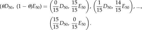When θ ≈ 1/2, these combination treatments correspond to over 90% inhibition of the bacterial population density relative to a control in which no drug is used [24].

Two controls were included: (i) M9 without antibiotics and without inoculation as a reference for density measurements and (ii) M9 (with glucose) without antibiotics but with inoculation to serve as the uninhibited growth reference. All treatments and controls were replicated 19 times, all plates were pipetted simultaneously.

Each one of the prepared microtitre plates was stored at 4°C until used. To control against drug degradation, a further plate was prepared and stored with the other plates for the duration of the 5-day experiment. At the end of the experiment, this plate was inoculated with an overnight culture of the original colony and measured for 24 h. Both on day 1 and when using this control plate, doxycycline and erythromycin caused a reduction of the AUC with no observed significant differences between these plates. This is consistent with maintenance of the efficacy of the drugs while in cold storage.

Appendix B. Optical density versus live cell counts

In order to demonstrate that measuring optical density at 600 nm in our shaken plate reading devices corresponds to counting live cells densities, we refer to the electronic supplementary material, figure S23, of [24]. This shows a linear correlation between the so-called colony forming units (CFU) and optical density (OD₆₀₀).

CFUs measure bacterial population densities by diluting a large bacterial population grown in liquid medium a number of times until single colonies can be determined when culturing those dilutions on agar plates, whence the name. So, ‘bacterial population density’ can be measured equivalently in CFUs per millilitre or in units of OD₆₀₀ according to the electronic supplementary material, figure S23, of [24] which shows a linear correlation between both cell density measures.

Appendix C. Model parameters

Tables 1 and 2.

Table 1.

Parameter values for E. coli strain AG100.

parameter	description	value
S0	glucose supply	2000 μg ml−1
D0	basal concentration of drug D	0.3 μg ml−1
E0	basal concentration of drug E	7 μg ml−1
	maximal carbon uptake rate
	of bacterial type i (μg cell−1 h−1)
K	bacterial half-saturation constant	0.0527 μg ml−1
c	resource conversion	2.18×104 cell μg−1
d	drug D binding rate	1.469×10−9 μg cell−1
e	drug E binding rate	1.44×10−9 μg cell−1
	inhibition of Bs (ml µg−1, ml µg−1, (ml µg−1)2, resp.)
	inhibition of Be (ml µg−1, ml µg−1, (ml µg−1)2, resp.)
	inhibition of Bd (ml µg−1, ml µg−1, (ml µg−1)2, resp.)
	inhibition of Bm (ml µg−1, ml µg−1, (ml µg−1)2, resp.)
ε	rate of point mutations	10−4 per locus per cell per division
η	dilution parameter	1% of biomass

Table 2.

Parameter values for E. coli strain MC4100.

parameter	description	value
S0	glucose supply	2000 μg ml−1
D0	basal concentration of drug D	0.15 μg ml−1
E0	basal concentration of drug E	9 μg ml−1
	maximal carbon uptake rate
	of bacterial type i (μg cell−1 h−1)
K	bacterial half-saturation constant	0.0527 μg ml−1
c	resource to biomass conversion	2.851×104 cell μg−1
d	drug D binding rate	1.469×10−9 μg cell−1
e	drug E binding rate	1.44×10−9 μg cell−1
	inhibition of Bs (ml µg−1, ml µg−1, (ml µg−1)2, resp.)
	inhibition of Be (ml µg−1, ml µg−1, (ml µg−1)2, resp.)
	inhibition of Bd (ml µg−1, ml µg−1, (ml µg−1)2, resp.)
	inhibition of Bm (ml µg−1, ml µg−1, (ml µg−1)2, resp.)
ε	rate of point mutations	10−4 per locus per cell per division
η	dilution parameter	1% of biomass

References

- 1.Levy AB, Marshall B. 2004. Antibacterial resistance worldwide: causes, challenges and responses. Nat. Med. 10, S122–S129. ( 10.1038/nm1145) [DOI] [PubMed] [Google Scholar]
- 2.Boucher HW, Talbot GH, Bradley JS, Edwards JE, Gilbert D, Rice LB, Scheld M, Spellberg B, Bartlett J. 2009. Bad bugs, no drugs: no ESKAPE! An update from the infectious diseases society of America. Clin. Infect. Dis. 48, 1–12. ( 10.1086/595011) [DOI] [PubMed] [Google Scholar]
- 3.Clatworthy AE, Pierson E, Hung DT. 2007. Targeting virulence: a new paradigm for antimicrobial therapy. Nat. Chem. Biol. 3, 541–548. ( 10.1038/nchembio.2007.24) [DOI] [PubMed] [Google Scholar]
- 4.von Gunten V, Reymond JP, Boubaker K, Gerstel E, Eckert P, Lüthi JC, Troillet N. 2009. Antibiotic use: is appropriateness expensive? J. Hosp. Infect. 71, 108–111. ( 10.1016/j.jhin.2008.10.026) [DOI] [PubMed] [Google Scholar]
- 5.Livermore D. 2004. Can better prescribing turn the tide of resistance? Nat. Rev. Microbiol. 2, 73–78. ( 10.1038/nrmicro798) [DOI] [PubMed] [Google Scholar]
- 6.Payne DJ. 2008. Microbiology: desperately seeking new antibiotics. Science 321, 1644–1645. ( 10.1126/science.1164586) [DOI] [PubMed] [Google Scholar]
- 7.Spellberg B, Powers JH, Brass EP, Miller LG, Edwards JE. 2004. Trends in antimicrobial drug development: implications for the future. Clin. Infect. Dis. 38, 1279–1286. ( 10.1086/420937) [DOI] [PubMed] [Google Scholar]
- 8.Alp E, van der Hoeven JG, Verweij PE, Mouton JW, Voss A. 2005. Duration of antibiotic treatment: are even numbers odd? J. Antimicrob. Chemother. 56, 441–442. ( 10.1093/jac/dki213) [DOI] [PubMed] [Google Scholar]
- 9.Roberts JA, Kruger P, Paterson DL, Lipman J. 2008. Antibiotic resistance: what's dosing got to do with it? Crit. Care Med. 36, 2433–2440. ( 10.1097/CCM.0b013e318180fe62) [DOI] [PubMed] [Google Scholar]
- 10.Pugh R, Grant C, Cooke RPD, Dempsey G. 2011. Short-course versus prolonged-course antibiotic therapy for hospital-acquired pneumonia in critically ill adults. Cochrane Database Syst. Rev ., CD007577 ( 10.1002/14651858.CD007577.pub2) [DOI] [PubMed] [Google Scholar]
- 11.Martinez MN, Papich MG, Drusano GL. 2012. Dosing regimen matters: the importance of early intervention and rapid attainment of the pharmacokinetic/pharmacodynamic target. Antimicrob. Agents Chemother. 56, 2795–2805. ( 10.1128/AAC.05360-11) [DOI] [PMC free article] [PubMed] [Google Scholar]
- 12.Geli P, Laxminarayan R, Dunne M, Smith DL. 2012. ‘One-size-fits-all’? Optimizing treatment duration for bacterial infections. PLoS ONE 7, e29838 ( 10.1371/journal.pone.0029838) [DOI] [PMC free article] [PubMed] [Google Scholar]
- 13.Taubes G. 2008. The bacteria fight back. Science 321, 356–361. ( 10.1126/science.321.5887.356) [DOI] [PubMed] [Google Scholar]
- 14.Tabor E. 2008. Bacteria by the book. Science 322, 853–854. ( 10.1126/science.322.5903.853b) [DOI] [PubMed] [Google Scholar]
- 15.Rice LB. 2008. Bacteria by the book: response. Science 322, 853–854. ( 10.1126/science.322.5903.853b) [DOI] [PubMed] [Google Scholar]
- 16.Huijben S, Bell AS, Sim DG, Tomasello D, Mideo N, Day T, Read AF. 2013. Aggressive chemotherapy and the selection of drug resistant pathogens. PLoS Pathog. 9, e1003578 ( 10.1371/journal.ppat.1003578) [DOI] [PMC free article] [PubMed] [Google Scholar]
- 17.1913. Address in pathology on chemotherapeutics. Lancet 182, 445–451. (Originally published as volume 2, issue 4694). ( 10.1016/S0140-6736(01)38705-6) [DOI] [Google Scholar]
- 18.Dancer SJ. 2004. How antibiotics can make us sick: the less obvious adverse effects of antimicrobial chemotherapy. Lancet Infect. Dis. 4, 611–619. ( 10.1016/S1473-3099(04)01145-4) [DOI] [PubMed] [Google Scholar]
- 19.Kalghatgi S, Spina CS, Costello JC, Liesa M, Morones-Ramirez JR, Slomovic S, Molina A, Shirihai OS, Collins JJ. 2013. Bactericidal antibiotics induce mitochondrial dysfunction and oxidative damage in mammalian cells. Sci. Transl. Med. 5, 192ra85 ( 10.1126/scitranslmed.3006055) [DOI] [PMC free article] [PubMed] [Google Scholar]
- 20.Sullivan A, Edlund C, Nord CE. 2001. Effect of antimicrobial agents on the ecological balance of human microflora. Lancet Infect. Dis. 1, 101–114. ( 10.1016/S1473-3099(01)00066-4) [DOI] [PubMed] [Google Scholar]
- 21.Fitzgerald JB, Schoeberl B, Nielsen UB, Sorger PK. 2006. Systems biology and combination therapy in the quest for clinical efficacy. Nat. Chem. Biol. 2, 458–466. ( 10.1038/nchembio817) [DOI] [PubMed] [Google Scholar]
- 22.Greco WR, Bravo G, Parsons JC. 1995. The search for synergy: a critical review from a response surface perspective. Pharmacol. Rev. 47, 331–385. [PubMed] [Google Scholar]
- 23.Read AF, Day T, Huijben S. 2011. The evolution of drug resistance and the curious orthodoxy of aggressive chemotherapy. Proc Natl Acad. Sci. USA 108(Suppl. 2), 10 871–10 877. ( 10.1073/pnas.1100299108) [DOI] [PMC free article] [PubMed] [Google Scholar]
- 24.Pena-Miller R, Laehnemann D, Jansen G, Fuentes-Hernandez A, Rosenstiel P, Schulenburg H, Beardmore R. 2013. When the most potent combination of antibiotics selects for the greatest bacterial load: the smile–frown transition. PLoS Biol. 11, e1001540. [DOI] [PMC free article] [PubMed] [Google Scholar]
- 25.Hegreness M, Shoresh N, Damian D, Hartl D, Kishony R. 2008. Accelerated evolution of resistance in multidrug environments. Proc. Natl Acad. Sci. USA 105, 13 977–13 981. ( 10.1073/pnas.0805965105) [DOI] [PMC free article] [PubMed] [Google Scholar]
- 26.Yeh PJ, Hegreness MJ, Aiden AP, Kishony R. 2009. Drug interactions and the evolution of antibiotic resistance. Nat. Rev. Microbiol. 7, 460–466. ( 10.1038/nrmicro2133) [DOI] [PMC free article] [PubMed] [Google Scholar]
- 27.Deresinski S. 2009. Vancomycin in combination with other antibiotics for the treatment of serious methicillin-resistant Staphylococcus aureus infections. Clin. Infect. Dis. 49, 1072–1079. ( 10.1086/605572) [DOI] [PubMed] [Google Scholar]
- 28.Bayer AS, Morrison JO. 1984. Disparity between timed-kill and checkerboard methods for determination of in vitro bactericidal interactions of vancomycin plus rifampin versus methicillin-susceptible and -resistant Staphylococcus aureus. Antimicrob. Agents Chemother. 26, 220–223. ( 10.1128/AAC.26.2.220) [DOI] [PMC free article] [PubMed] [Google Scholar]
- 29.Howe RA, Andrews JM. 2012. BSAC standardized disc susceptibility testing method (version 11). J. Antimicrob. Chemother. 67, 2783–2784. ( 10.1093/jac/dks391) [DOI] [PubMed] [Google Scholar]
- 30.Amsterdam D. 2005. Susceptibility testing of antimicrobials in liquid media. In Antibiotics in laboratory medicine, 5th edn (ed. Lorian V.), pp. 61–143. Philadelphia, PA: Lippincott Williams and Wilkins; (http://books.google.ca/books?id=HdA4dl8m\_T4C\&printsec=front cover\&source=gbs\_ge\_summary \_r\&cad=0\#v=onepage\& q\&f=false). [Google Scholar]
- 31.Peña Miller R, Lähnemann D, Schulenburg H, Ackermann M, Beardmore RE. 2012. Selecting against antibioticresistant pathogens: optimal treatments in the presence of commensal bacteria. Bull. Math. Biol. 74, 908–934. ( 10.1007/s11538-011-9698-5) [DOI] [PubMed] [Google Scholar]
- 32.Peña Miller R, Lähnemann D, Schulenburg H, Ackermann M, Beardmore RE. 2012. The optimal deployment of synergistic antibiotics: a control-theoretic approach. J. R. Soc. Interface 9, 2488–2502. ( 10.1098/rsif.2012.0279) [DOI] [PMC free article] [PubMed] [Google Scholar]
- 33.Chou TC, Talalay P. 1981. Generalized equations for the analysis of inhibitions of Michaelis–Menten and higherorder kinetic systems with two or more mutually exclusive and nonexclusive inhibitors. Eur. J. Biochem. 115, 207–216. ( 10.1111/j.1432-1033.1981.tb06218.x) [DOI] [PubMed] [Google Scholar]
- 34.Andersson DI, Levin BR. 1999. The biological cost of antibiotic resistance. Curr. Opin. Microbiol. 2, 489–493. ( 10.1016/S1369-5274(99)00005-3) [DOI] [PubMed] [Google Scholar]
- 35.Ochman H, Lawrence JG, Groisman Ea. 2000. Lateral gene transfer and the nature of bacterial innovation. Nature 405, 299–304. ( 10.1038/35012500) [DOI] [PubMed] [Google Scholar]
- 36.Weinreich DM, Delaney NF, Depristo MA, Hartl DL. 2006. Darwinian evolution can follow only very few mutational paths to fitter proteins. Science 312, 111–114. ( 10.1126/science.1123539) [DOI] [PubMed] [Google Scholar]
- 37.Sandegren L, Andersson DI. 2009. Bacterial gene amplification: implications for the evolution of antibiotic resistance. Nat. Rev. Microbiol. 7, 578–588. ( 10.1038/nrmicro2174) [DOI] [PubMed] [Google Scholar]
- 38.Wheat PF. 2001. History and development of antimicrobial susceptibility testing methodology. J. Antimicrob. Chemother. 48(Suppl. 1), 1–4. ( 10.1093/jac/48.suppl_1.1) [DOI] [PubMed] [Google Scholar]
- 39.Kahlmeter G, et al. 2006. European committee on antimicrobial susceptibility testing (EUCAST) technical notes on antimicrobial susceptibility testing. Clin. Microbiol. Infect. 12, 501–503. ( 10.1111/j.1469-0691.2006.01454.x) [DOI] [PubMed] [Google Scholar]
- 40.Eagle H, Musselman AD. 1948. The rate of bactericidal action of penicillin in vitro as a function of its concentration, and its paradoxically reduced activity at high concentrations against certain organisms. J. Exp. Med. 88, 99–131. ( 10.1084/jem.88.1.99) [DOI] [PMC free article] [PubMed] [Google Scholar]
- 41.Odds FC. 2003. Synergy, antagonism, and what the chequerboard puts between them. J. Antimicrob. Chemother. 52, 1 ( 10.1093/jac/dkg301) [DOI] [PubMed] [Google Scholar]
- 42.WHO Library Cataloguing-in-Publication Data: Treatment of tuberculosis: guidelines, 4th edn; 2012 See http://whqlibdoc.who.int/publications/2010/9789241547833\_eng.pdf (accessed 5 April 2012).
- 43.Kim YS, et al. 2011. Randomised clinical trial: the efficacy of a 10-day sequential therapy vs. a 14-day standard proton pump inhibitor-based triple therapy for Helicobacter pylori in Korea. Aliment. Pharmacol. Ther. 34, 1098–1105. ( 10.1111/j.1365-2036.2011.04843.x) [DOI] [PubMed] [Google Scholar]
- 44.Vaira D, Zullo A, Hassan C, Fiorini G, Vakil N. 2009. Sequential therapy for Helicobacter pylori eradication: the time is now! Therap. Adv. Gastroenterol. 2, 317–322. ( 10.1177/1756283X09343326) [DOI] [PMC free article] [PubMed] [Google Scholar]
- 45.Greenberg ER, et al. 2011. 14-day triple, 5-day concomitant, and 10-day sequential therapies for Helicobacter pylori infection in seven Latin American sites: a randomised trial. Lancet 378, 507–514. ( 10.1016/S0140-6736(11)60825-8) [DOI] [PMC free article] [PubMed] [Google Scholar]
- 46.Bergeron M, Ouellette M. 1998. Preventing antibiotic resistance through rapid genotypic identification of bacteria and of their antibiotic resistance genes in the clinical microbiology laboratory. Clin. Microbiol. 36, 2169–2172. [DOI] [PMC free article] [PubMed] [Google Scholar]
- 47.Bergeron MG, Ouellette M. 1998. Preventing antibiotic resistance using rapid DNA-based diagnostic tests-based diagnostic tests. Infect. Control Hosp. Epidemiol. 19, 560–564. ( 10.2307/30141780) [DOI] [PubMed] [Google Scholar]
- 48.MacDougall C, Polk RE. 2005. Antimicrobial stewardship programs in health care systems. Clin. Microbiol. Rev. 18, 638–656. ( 10.1128/CMR.18.4.638-656.2005) [DOI] [PMC free article] [PubMed] [Google Scholar]
Associated Data
This section collects any data citations, data availability statements, or supplementary materials included in this article.
Data Availability Statement