Selectivity for space and time in early areas of the auditory dorsal stream in the rhesus monkey

Abstract

The respective roles of ventral and dorsal cortical processing streams are still under discussion in both vision and audition. We characterized neural responses in the caudal auditory belt cortex, an early dorsal stream region of the macaque. We found fast neural responses with elevated temporal precision as well as neurons selective to sound location. These populations were partly segregated: Neurons in a caudomedial area more precisely followed temporal stimulus structure but were less selective to spatial location. Response latencies in this area were even shorter than in primary auditory cortex. Neurons in a caudolateral area showed higher selectivity for sound source azimuth and elevation, but responses were slower and matching to temporal sound structure was poorer. In contrast to the primary area and other regions studied previously, latencies in the caudal belt neurons were not negatively correlated with best frequency. Our results suggest that two functional substreams may exist within the auditory dorsal stream.

ever since the proposition of a dual-stream model of cortical processing in vision (Mishkin et al. 1983; Ungerleider and Mishkin 1982), and the later adoption of a related model for audition (Rauschecker 1997, 1998; Romanski et al. 1999a, 1999b; Tian et al. 2001), the model has faced both challenges and modifications. The role of the dorsal processing stream has been debated most intensely. In the visual system, for example, it has been proposed that the function of the dorsal stream is primarily to support visually guided action (“how”; Goodale and Milner 1992) rather than the originally assigned computation of stimulus location in space (“where”; Ungerleider and Mishkin 1982). Recently, Kravitz et al. (2011) presented a model of the visual dorsal stream wherein three different functions (spatial working memory, visually guided actions, and spatial navigation) are performed by anatomically distinct components of the dorsal stream, all originating from parietal cortex. Similarly, there have been attempts to redefine the roles of auditory processing streams, in particular the dorsal stream, which was originally assumed to deal mainly with the spatial location of sounds (“where”) and their motion in space (Rauschecker and Tian 2000). Early on, Belin and Zatorre (2000) argued for the stream's role in tracking of spectral motion and, consequently, in speech recognition (again termed a “how”-stream), while Schubotz et al. (2003) described segregation of auditory “where” and “when” (timing of acoustic rhythm) at a later stage of dorsal stream processing, in lateral premotor cortex. Kaas and Hackett (1999) mentioned the possibility of substreams or streamlets and noted anatomical evidence for more than two pathways originating from auditory cortex (Kaas and Hackett 2000).

Converging support for the role of the auditory dorsal stream in sound localization came from anatomical (Kaas and Hackett 2000; Romanski et al. 1999a, 1999b) and electrophysiological (Miller and Recanzone 2009; Recanzone et al. 2000a; Tian et al. 2001; Woods et al. 2006; Zhou and Wang 2012) studies in nonhuman primates and from neuroimaging studies in humans (e.g., Arnott et al. 2004; Krumbholz et al. 2005a, 2005b; Maeder et al. 2001; Warren et al. 2002; see Rauschecker 2007, 2012 for review). However, other studies in humans have provided evidence for various nonspatial auditory functions to be represented in areas currently assumed to belong to the dorsal stream as well. These have included speech processing (Dhanjal et al. 2008; Geschwind 1965; Hickok et al. 2009; Wernicke 1874; Wise et al. 2001; see, however, DeWitt and Rauschecker 2012), tracking of spectral motion (Belin and Zatorre 2000), timing of acoustic rhythm (Schubotz et al. 2003), singing (Perry et al. 1999), imagery of music (Leaver et al. 2009), and representation of tool sounds (Lewis et al. 2005). It has been argued that these functions are specific manifestations of a more general function of audio-motor control, which includes the processing of space and motion in space (Rauschecker 2011; Rauschecker and Scott 2009).

The auditory dorsal stream of nonhuman primates originates from the caudal belt (Kaas and Hackett 2000; Romanski et al. 1999a, 1999b). Connections of the caudal belt (and of neighboring areas of the posterior temporal lobe) with the dorsolateral regions of prefrontal, premotor, and posterior parietal cortex have been reported (Lewis and Van Essen 2000; Morecraft et al. 2012; Romanski et al. 1999a, 1999b; Smiley et al. 2007; Ward et al. 1946). These regions are implicated in the proposed model of the auditory dorsal stream (Rauschecker 2011, 2012). Two components of the caudal belt, the caudomedial (CM) and caudolateral (CL) areas, differ in their thalamo-cortical and cortico-cortical connectivity (Hackett et al. 2007; Smiley et al. 2007); it is therefore of interest to study whether (and how) they differ in neural response properties as well. In the context of the putative role of the dorsal stream, spatial selectivity and temporal accuracy of neural responses are of particular interest. So far, however, electrophysiological studies in the caudal belt have focused more on the former (Miller and Recanzone 2009; Recanzone et al. 2000a; Tian et al. 2001; Woods et al. 2006; Zhou and Wang 2012) and less on the latter (see, however, Oshurkova et al. 2008; Scott et al. 2011).

The internal structure and possible division of labor within the caudal belt, which could shed light on the functional organization of the early dorsal stream, should be ideally investigated by direct comparison of physiological properties of CM and CL in the same animals. This has rarely been the case; in many studies only one of these areas was investigated, areas were pooled together, or CM was studied in different animals from CL (Camalier et al. 2012; Oshurkova et al. 2008; Recanzone et al. 2000a; Scott et al. 2011; Tian et al. 2001; Zhou and Wang 2012). So far, the two areas have been compared directly only in one set of monkeys, showing enhanced spatial selectivity in the horizontal plane in CL but not CM (Miller and Recanzone 2009; Woods et al. 2006). This result suggests that the spatial function of the dorsal stream might be limited to only a part of the caudal belt. However, even if this is correct, it remains unknown whether CL's superior spatial selectivity (compared with CM) is limited to azimuth or applies to elevation as well.

The temporal properties of the caudal belt are even less clear. The ability to precisely follow rapid temporal changes of acoustic stimuli gradually diminishes from A1 to more rostral areas (e.g., Bendor and Wang 2008; Kuśmierek and Rauschecker 2009; Scott et al. 2011). It is currently unclear whether temporal precision also diminishes caudal to A1 (i.e., shows a gradient reversal) or the same gradient continues, leading to temporal locking to even faster changes in the caudal belt. Locking to fast temporal modulations has been reported to be either poorer (Oshurkova et al. 2008) or similar or better (Scott et al. 2011) in CM compared with A1. Response latencies have been shown to be either similar in A1 and CM (Oshurkova et al. 2008; Recanzone et al. 2000b) or shorter in CM (Camalier et al. 2012; Kajikawa et al. 2005; Scott et al. 2011).

In this study, we characterized areas CM and CL of the same animals, using multiple response properties. In particular, we analyzed spatial selectivity (in both azimuth and elevation) and temporal factors (response latency and temporal accuracy). Our results show that there is a segregation between CL and CM in latency and temporal accuracy vs. spatial selectivity, which suggests that dorsal stream regions may be specialized for distinct roles already at the level of the caudal belt.

MATERIALS AND METHODS

Animals.

The study was conducted in three male adult rhesus monkeys (monkeys B, M, and N), each implanted with an elongated (19 mm × 38 mm) plastic recording chamber (Crist Instruments, Hagerstown, MD) in approximately antero-posterior orientation over auditory areas and a headpost. Implants were placed and recordings were conducted in the left hemisphere, which may affect the generality of results, should the studied functions be strongly lateralized. Implantation was guided and later confirmed by 3-T 1-mm³-voxel size MRI. The animals were water-restricted to ensure adequate drive in a fluid-rewarded task. The age of monkeys during the recordings was 8–10 yr for monkeys M and N and ∼12 yr for monkey B (monkey B was born from a free-ranging colony, and the date of birth is approximate). The experiments were approved by the Georgetown University Animal Care and Use Committee.

Task and stimuli.

Monkeys were seated and head-fixed in a monkey chair (Crist Instruments) in a 2.6 m × 2.6 m × 2.0 m (W × L × H) sound-attenuated chamber (IAC, Bronx, NY). To ensure attention, the animals were working in a go/no-go auditory discrimination task throughout the experiment. Touchbar-release responses to infrequent target stimuli [300-ms white noise (WN) bursts] were rewarded with small amounts of fluid.

In addition to WN bursts, 35 other stimuli were used. Twenty-one artificial sounds comprised pure tones (PT), ⅓-octave band-pass noise bursts (BPN), and 1-octave BPN, seven each. The frequencies of PT and BPN were 1-octave spaced from 250 Hz to 16 kHz. [Throughout this article, “BPN frequency” denotes BPN center frequency; similarly, “best frequency” (BF) means best center frequency when applied to BPN bursts.] Two classes of natural stimuli (14 total) were also used to assess selectivity for natural sounds: seven monkey calls (MC) and seven environmental sounds (ES). Duration of PT and BPN stimuli was 300 ms, while MC and ES ranged between 150 and 1,706 ms (Kuśmierek et al. 2012). ES were recorded in our animal facility and were therefore likely familiar and meaningful to the monkeys. MC were obtained from a digital library provided by Marc Hauser (Hauser 1998). Spectrograms of the natural stimuli are shown in Fig. 1. All stimuli were presented at 42 dB above the macaque hearing threshold (Jackson et al. 1999); see Kuśmierek and Rauschecker (2009) for measurement and level-equalizing method. Unweighted sound pressure level of the stimuli ranged from 43.8 to 56.4 dB sound pressure level (SPL) for PT and BPN, from 44.9 to 49.8 dB SPL for MC, and from 45.5 to 48.3 dB SPL for ES. Digitized stimuli (48-kHz sampling frequency, 16-bit resolution) were played with a Power1401 MkII laboratory interface (CED, Cambridge, UK), a PA4 attenuator (TDT, Alachua, FL), a SE 120 amplifier (Hafler, Tempe, AZ), and 400-312-10 3.5-in. one-way speakers (CTS, Elkhart, IN). The speakers were arranged in a vertical arc-shaped array (Crist Instruments) that was rotated around the monkey chair with a Unidex 100 controller (Aerotech, Pittsburgh, PA) and a 300SMB3-HM (Aerotech) stepper motor. This allowed for manipulation of the azimuth of the sound source. An ROB-24 Relay Output Card (Acces IO Products, San Diego, CA) controlled via a custom-built demultiplexer was used to select one speaker of the array and thus control the elevation of the sound source. The experiment was controlled by the Power1401 interface and Spike2 program (v.6 or 7, CED) running custom-made scripts. The distance between the loudspeakers and the monkey's head was ∼0.95 m.

Fig. 1.

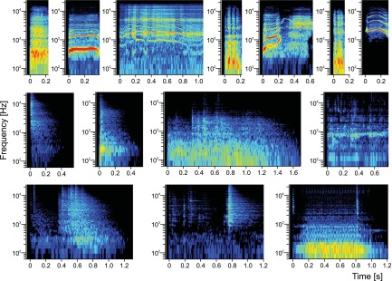
Spectrograms of monkey calls (MC) and environmental sounds (ES) used in the study. Top: MC: bark, coo, girney, grunt, harmonic arch, pant threat, scream. Middle and bottom: ES: cage latch, monkey chair latch opening, moving food container, water dripping, padlock open, monkey pole latch, vacuum pump.

Neural recordings.

Single-unit and multiunit recordings were obtained by advancing one to four Epoxylite- or glass-insulated 1- to 3-MΩ tungsten electrodes (FHC, Bowdoin, ME, or NAN Instruments, Nazareth Illit, Israel) into the auditory cortex by means of a micropositioner (model 650, David Kopf, Tujunga, CA, or FlexMT/EPS, Alpha Omega, Nazareth Illit, Israel). A stainless steel guide tube was used to puncture the dura. A 1 mm × 1 mm spacing grid provided a repeatable spatial reference for electrode location. When more than one electrode was used, each electrode was inserted in a separate grid location. The electrode signal was amplified and filtered (model 1800, A-M Systems, Sequim, WA and PC1, TDT; or MCP Plus, Alpha Omega) and sampled by the Power1401 interface using the Spike2 program and custom-made scripts. The location of auditory cortex was determined from recording depth (in reference to MRI images), from the presence of a “silent gap” corresponding to the lateral sulcus, and from auditory responses of the neurons. Only auditory-responsive units were tested further.

Recording session design.

Each daily experiment consisted of several stages. In the search stage, the speaker array was positioned at 0° azimuth (in front of the monkey) and all stimuli were played at five elevations of −60°, −30°, 0°, 30°, and 60° while the electrode(s) was advanced until responsive auditory neurons were found and isolated, as determined by online observation of responses to played stimuli or to natural stimuli produced ad hoc (knocking, clapping, etc.). In stage A of the actual recording session (stage of the experiment in which azimuth sensitivity was studied), a subset of stimuli [white noise + PT + ⅓-octave BPN (in some cases PT stimuli were omitted)] was presented at different azimuths and an elevation of 0°. To reduce the possible systematic influence of recording drift, the array location during the stage was set consecutively at eight locations from 0° to 315° in 45° steps in counterclockwise order and then back clockwise from 315° to 0°. In about half of the experiments, clockwise motion (8 locations in the order 0° to 45°) was used first, followed by counterclockwise return (45° to 0°). On the basis of online template-sorted neural activity, the best azimuth was estimated from data collected in stage A, typically as the azimuth at which activity to the preferred stimulus was highest in any of the 20-ms bins within the first 100 ms of the response. In the second stage (stage E, stage of the experiment in which elevation sensitivity was studied), the complete set of stimuli was presented at the best azimuth and at five elevations of −60°, −30°, 0°, 30°, and 60°. In all stages the stimuli were arranged in blocks, in which WN was played three to seven times at each elevation used in the stage and each of the other stimuli was played once at each elevation. Stimulus order within the block was randomized, and 12 blocks were played both in stage E and at each azimuth location of stage A (split 6:6 between the clockwise and counterclockwise runs). Thus in stage A each stimulus (except WN and stimuli not used in this stage) was played 96 times (12 times at each of 8 azimuths), while in stage E each of the stimuli (except WN) was played 60 times (12 times at each of 5 elevations).

Cortical areas.

The recorded units were assigned to one of three cortical areas: A1, CM, and CL. First, the A1/caudal belt boundary was delineated based on the average BF of recording locations. For each unit, BF was determined by first averaging (on a logarithmic scale) the BF derived from response to PT (see further below for the method) and BPN, separately for stages A and E, and then averaging the values from the two stages. Next, values from all units recorded at the same grid location were averaged to create raw BF maps and, by smoothing with a Gaussian kernel (σ = 0.5 mm), smoothed BF maps (Fig. 2). In the smoothed map, maximum BF in each row (i.e., in antero-posterior direction) was found, and the A1/caudal belt boundary was placed either immediately anterior or immediately posterior to the location of maximum BF, on the side where the adjacent location's BF was higher. All units anterior to the boundary were assigned to area A1; no attempt was made to distinguish the middle medial (MM) or middle lateral (ML) areas adjacent to A1, and no obvious signs were seen that the recording area included any of these belt regions. Posterior to the A1/caudal belt boundary, units were assigned to CM or CL on the basis of physical location on the superior temporal plane. Histological data are not available for these monkeys' brains, and we decided to avoid using electrophysiologically determined differences between the areas (see results) for area delineation to prevent any circular reasoning. However, one of the outcomes of this study is identification of neural response properties that may be useful to tell CM apart from CL in future studies. With structural MRI images, the boundaries of the superior temporal plane (STP; medially: the fundus of the lateral sulcus, laterally: the lip of the lateral sulcus) were determined. Units in the medial half of the STP were assigned to CM and those on the lateral half to CL. Anatomical studies often find the boundary between CM and CL to run approximately in the center of the STP (Hackett et al. 1998; Smiley et al. 2007). All caudal belt units recorded in monkey B were assigned to CM, whereas in monkeys N and M both CM and CL were represented. In addition, structural MRI images were aligned to the 112RM-SL_T1 rhesus monkey template (McLaren et al. 2009), and recording areas were checked against the rhesus monkey brain atlas (Saleem and Logothetis 2007) associated with the template. The electrophysiological data were tested against uncertainty of the CM/CL boundary location by replicating the analyses with recording locations adjacent to the boundary on both sides dropped. Because no CL units were recorded from monkey B, the analyses were also replicated with data from monkeys N and M only. In both tests, only a few minor differences from results based on the complete data set were found (Table 1).

Fig. 2.

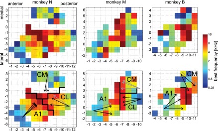
Maps of best (center) frequencies (BF) in all 3 monkeys; recording grid coordinates in millimeters. Top: raw data. Bottom: data smoothed with Gaussian kernel (σ = 0.5 mm). Cortical area boundaries and designations are drawn in black. In monkey N (left) several locations in the lateral part of caudomedial area (CM) were not recorded from because of a large blood vessel detected in the MRI images. Arrows show direction of cochleotopic gradients (low to high BF) detected in each area. Black arrows indicate significant gradients (P < 0.05) and gray arrows nonsignificant gradients. Three arrows per area show results obtained with 3 stimulus bandwidths: pure tones (PT), ⅓-octave band-pass noise (BPN), and 1-octave BPN. CL, caudolateral area.

Table 1.

Results of statistical tests

Test/comparison	Figure	Areas Compared	P Value Obtained with Full Data Set	P Value with Boundary-Adjacent Units Dropped	Difference	P Value with Monkey B Dropped	Difference
Frequency PI for PT	3	ANOVA	6.4 × 10−6	7.4 × 10−6		0.00036
		A1 vs. CM	0.048	0.17	−	0.042
		A1 vs. CL	2.4 × 10−6	2.6 × 10−6		0.00025
		CM vs. CL	0.048	0.015		0.46	−
Frequency PI for ⅓-oct BPN	3	ANOVA	0.00014	3.4 × 10−5		0.0044
		A1 vs. CM	0.019	0.047		0.038
		A1 vs. CL	8.0 × 10−5	1.0 × 10−5		0.0054
Frequency PI for 1-oct BPN	3	ANOVA	0.032	0.011		0.12	−
		A1 vs. CL	0.031	0.0072		0.19	−
Linear discriminator performance for PT	3	ANOVA	0.00039	0.00063		0.00025
		A1 vs. CL	5.2 × 10−5	0.00014		5.9 × 10−5
Linear discriminator performance for ⅓-oct BPN	3	ANOVA	0.00052	0.00068		0.0010
		A1 vs. CL	5.3 × 10−5	6.2 × 10−5		0.00019
		CM vs. CL	0.0095	0.013		0.023
Linear discriminator performance for 1-oct BPN	3	ANOVA	2.7 × 10−5	4.3 × 10−5		2.3 × 10−5
		A1 vs. CL	1.1 × 10−6	1.5 × 10−6		3.7 × 10−6
		CM vs. CL	0.01	0.0097		0.04
Number of peaks in frequency-rate curve, PT	3	ANOVA	0.00083	0.00040		0.0021
		A1 vs. CM	0.0071	0.0081		0.007
		A1 vs. CL	0.0015	0.00062		0.0071
Number of peaks in frequency-rate curve, ⅓-oct BPN	3	ANOVA	0.029	0.048		0.014
		A1 vs. CM	0.033	0.16	−	0.014
Stimulus PI for MC	4	ANOVA	0.016	0.018		0.011
		A1 vs. CL	0.059	0.024	+	0.094
		A1 vs. CM	0.056	0.28		0.021	+
Stimulus PI for ES	4	ANOVA	0.017	0.061	−	0.026
		A1 vs. CL	0.041	0.1	−	0.05
Linear discriminator performance for MC	4	ANOVA	1.2 × 10−5	1.9 × 10−5		9.2 × 10−6
		A1 vs. CM	0.013	0.014		0.0063
		A1 vs. CL	1.5 × 10−5	2.8 × 10−5		1.8 × 10−5
Linear discriminator performance for ES	4	ANOVA	2.2 × 10−5	1.7 × 10−5		4.6 × 10−5
		A1 vs. CL	1.5 × 10−5	6.3 × 10−6		4.2 × 10−5
		CM vs. CL	0.00098	0.0011		0.0023
Azimuth PI, best PT	6	ANOVA	0.017	0.0015		0.018
		A1 vs. CL	0.0087	0.00092		0.0087
		CM vs. CL	0.31	0.017	+	0.4
Azimuth PI, best ⅓-oct BPN	6	ANOVA	0.034	0.0073		0.066	−
		A1 vs. CL	0.035	0.0084		0.13	−
		CM vs. CL	0.096	0.023	+	0.11
Azimuth PI, WN	6	ANOVA	0.017	0.00022		0.017
		A1 vs. CL	0.038	0.0019		0.038
		CM vs. CL	0.027	0.00027		0.027
Elevation PI, best 1-oct BPN	6	ANOVA	0.012	0.014		0.027
		CM vs. CL	0.0085	0.013		0.017
Elevation PI, wide band averaged	6	ANOVA	0.019	0.023		0.071	−
		CM vs. CL	0.018	0.018		0.075	−
Latency	7	ANOVA	5.1 × 10−14	2.4 × 10−13		2.2 × 10−12
		A1 vs. CM	4.1 × 10−13	7.1 × 10−13		2.6 × 10−12
		CM vs. CL	1.7 × 10−9	1.5 × 10−8		1.7 × 10−7
Latency-best frequency correlation	7	A1	5.4 × 10−6	5.4 × 10−6		1.8 × 10−5
			r = −0.364	r = −0.364		r = −0.386
		CM	0.44	0.39		0.58
			r = −0.076	r = −0.091		r = −0.061
		CL	0.10	0.10		0.10
			r = −0.179	r = −0.202		r = −0.179
Linear discriminator best window, all stimuli	8	ANOVA	1.2 × 10−9	1.0 × 10−7		2.5 × 10−7
		A1 vs. CM	0.00089	0.00039		0.0010
		A1 vs. CL	0.0010	0.021		0.046
		CM vs. CL	2.2 × 10−9	2.8 × 10−7		5.6 × 10−7
Correlation between acoustic structure and firing rate, ES	9	ANOVA	0.019	0.039		0.053	−
		CL vs. CM	0.021	0.04		0.067	−

Values are results of statistical tests with units adjacent to the caudomedial (CM)/caudolateral (CL) boundary dropped to test against uncertainty of the boundary location, or with units recorded from monkey B dropped, compared to results obtained with the full data set. Except for latency-best frequency (BF) correlations, all P values are for pairwise comparisons between areas by t-test and corrected for multiple (3) comparisons with Šidak correction, or for ANOVA comparing all 3 areas. Analyses resulting in nonsignificant P value (P ≥ 0.05) for both full data set and with units dropped are not shown (except for latency-BF correlations). Difference is coded as “+” when dropping the units changed the P value from nonsignificant to significant and as “−”' when it changed the P value from significant to nonsignificant. For latency-BF correlation, r values are also provided.

PI: preference index; PT, pure tones; BPN, band-pass noise; MC, monkey calls; ES, environmental sounds; WN, white noise.

The total number of recorded units was 346, including 153 in A1 (monkey N: 66, M: 55, B: 32), 107 in CM (monkey N: 52, M: 35, B: 20), and 86 in CL (monkey N: 42, M: 44). In the test with recording locations adjacent to the CM/CL boundary removed, there were 92 CM units and 68 CL units.

Data analysis.

Most analysis methods are similar to those published recently (Kuśmierek et al. 2012; Kuśmierek and Rauschecker 2009). Data from monkeys B and (partially) N were also used previously in population analyses of the rostral auditory areas (Kuśmierek et al. 2012).

Recorded spikes were sorted off-line with the Spike2 program [typically using principal component analysis (PCA)], and spike timestamps were exported to MATLAB (MathWorks, Natick, MA) for further analysis with custom-made scripts. The timestamps were corrected for sound travel time from the loudspeaker to the monkey head (2.8 ms).

Several analyses were based on peak firing rate (PFR), defined as the maximum firing rate in a sliding 20-ms window (1-ms step) along the response averaged across stimulus repetitions (similar to Kuśmierek and Rauschecker 2009) over the entire stimulus duration (unless otherwise specified).

BF was determined by fitting a quadratic function to the frequency-PFR curve at the frequency where the highest PFR occurred and the two neighboring frequencies on either side; BF was assumed to be at the peak of the fitted function. If the highest PFR occurred at one of the outermost frequencies (0.25 or 16 kHz), this frequency was determined to be the BF. Log transformation was applied to sound frequency prior to any calculations. The number of peaks in the frequency-PFR curve was measured by counting the number of the curve's sections with PFR higher than 75% of the highest PFR separated by sections with PFR below or equal to that threshold.

Cochleotopic gradient direction and significance was determined in each area (separately for each monkey) in the same way as previously described (Kuśmierek and Rauschecker 2009). Briefly, we calculated the correlation coefficient (r) of average BF at each recording site with spatial locations of the site projected onto an axis that was rotated 360° with a 5° step. The rotation angle at which the maximum r was found indicated the direction of the gradient. Significance of the gradient was determined by comparing the maximum r to a distribution of maximum r values obtained from repeating the calculation 1,000 times with BF values randomly reassigned among the loci's spatial locations.

Stimulus selectivity was determined within class and at the level of individual units with the preference index (PI) and linear discriminator performance. PI is the fraction of stimuli in the class (other than the best stimulus, i.e., one that evoked the highest PFR) that elicited at least 50% of the PFR of the best stimulus (Kuśmierek and Rauschecker 2009), and it ranges from 0 (high selectivity) to 1 (low selectivity). In the of case of PT and ⅓-octave BPN, which were used in both stages A and E, the PI of a unit was calculated as the average of PIs calculated from each stage. PI was also used as a measure of spatial selectivity: here, instead of using PFR of various stimuli within a class, we used the PFR elicited by one stimulus at various azimuths or elevations. Spatial PI were calculated for WN, best PT, best ⅓-octave BPN, and, in the case of elevation, best 1-octave BPN. PI (whether for stimulus identity or for spatial position) was calculated only if at least one stimulus of the underlying class evoked an average firing rate significantly different from the average firing rate in the 200 ms preceding stimulus onset (P < 0.05, Wilcoxon test).

Linear discriminator analysis was performed as described previously (see Kuśmierek et al. 2012; Kuśmierek and Rauschecker 2009; Recanzone 2008; Russ et al. 2008 for details). For each unit and each stimulus class (PT, ⅓-octave BPN, 1-octave BPN, MC, and ES) we determined whether a single trial's spike train was more similar to combined remaining single spike trains elicited by the same stimulus (success) or to combined spike trains elicited by any other stimulus (failure). The similarity was determined by calculating Euclidean distance between spike trains binned with bin widths ranging from 2 to 500 ms. One outcome of the procedure was a measure of stimulus selectivity: linear discriminator performance, i.e., the highest proportion of successes of all bin widths. The bin width at which the highest performance was found (best bin width) was the second outcome, providing an estimate of the temporal accuracy with which responses to different presentations of the same stimulus were replicated. Only data from stage E, in which all five stimulus classes were used, were subjected to this analysis.

We analyzed the ability of neural populations in the three areas to discriminate between four a priori sound categories: low-frequency artificial sounds, high-frequency artificial sounds, MC, and ES. The method was described previously (Kuśmierek et al. 2012). Briefly, average firing rate for each neuron and stimulus was determined in eight 20-ms time bins covering the first 160 ms of the stimulus time and in a 20-ms bin preceding the stimulus (pretrial). Within every bin, each unit's response to the stimulus set was treated as a vector and normalized by subtracting the mean and dividing by the vector's Euclidean length. The responses were arranged into a units × stimuli matrix, and a k-means procedure was used to cluster stimuli into four categories based on responses of many units (“population response”), separately for each cortical area. Precautions were taken to ensure that the different number of units per area did not confound the result, and classification success for each area and time bin was evaluated statistically compared with pretrial as well as compared with a “reference range” created by randomly reassigning the neurons to regions and repeating the k-means analysis many times in an identical manner. The output measure was classification success at each bin, i.e., the proportion of stimuli that were clustered into their a priori categories.

The three selectivity measures used in this study addressed different aspects of stimulus selectivity. The PI and linear discriminator performance measured within-class selectivity of individual units. That is, for each unit we assessed whether it responded differentially to different stimuli within a class (PT, ⅓-octave or 1-octave BPN, MC, ES). The k-means classification success, on the other hand, estimated how well neural populations can distinguish between stimulus categories (low- and high-frequency artificial sounds, MC, ES). In addition, the measures addressed the temporal structure of the neural response differently. With PI, the temporal structure was disregarded. The k-means classification used firing rate averaged over short time bins, allowing us to capture changes of classification accuracy over time. Still, it was computed separately for each bin, so the procedure did not provide a single measure sensitive to temporal structure of neural responses. Linear discriminator performance, on the other hand, took the temporal structure of neural responses into account by using all temporal bins at once, and also by testing different bin sizes to find the most appropriate one.

To obtain neural response latencies, spike trains across all repetitions of a stimulus were binned with a 1-ms bin width and smoothed exponentially [y_i = αx_i + (1 − α)y_i−1, α = 0.3]. Neural latency was defined as the time of the first bin in which the smoothed value exceeded the average smoothed firing rate from the 250 ms preceding the stimulus onset by at least 2 SDs and remained above 2 SD for at least 10 ms (Kuśmierek and Rauschecker 2009). Separately for stages A and E, neural latency was determined as the shortest of the following: latency of the PT that elicited the highest PFR (“best PT”), latency of the best ⅓-octave BPN, latency of the best stimulus of PT, BPN, WN, and, in stage E, latency of the best 1-octave BPN. Finally, a unit's latency was the mean of latency values from the two stages.

We estimated the units' ability to follow the temporal acoustic structure of stimuli with pronounced temporal structure, that is, MC and ES. The estimate was the Pearson correlation coefficient between firing rate and acoustic energy. To account for frequency tuning, the stimuli were split into seven 1-octave-wide frequency bands (center frequencies 0.25–16 kHz) with a 16,384-point fast Fourier transform (FFT) finite impulse response (FIR) filter. For each band, RMS value was calculated in 1-ms bins and expressed in decibels relative to full digital scale (dBfs). Time stamps of spikes fired by a unit during all repetitions of a stimulus were binned at 1 ms after subtraction of neural latency. The Pearson correlation coefficient between the RMS time series and the spiking time series was calculated for each band, and the highest coefficient of all bands was taken as the estimate of the unit's ability to follow the stimulus acoustic structure. Finally, average correlation coefficients across all MC or all ES were used to compare this ability between cortical areas. This average was calculated using only stimuli that evoked an average firing rate significantly different from the average firing rate in the 200 ms preceding stimulus onset (P < 0.05, Wilcoxon test); if none of the stimuli of the class drove the unit significantly, the unit was dropped from the analysis.

Unless stated otherwise, statistical comparisons between areas were conducted with one-way ANOVAs, followed by pairwise t-tests with Šidak correction for multiple (3) comparisons. In most cases, results of the t-test are provided in the figures and results of the ANOVAs in the text. The significance criterion was P < 0.05. Note that calculation of many neural parameters was contingent on certain criteria; if the criteria were not met, the unit was rejected from the specific analysis. This is the reason why the number of units varies somewhat between analyses (as apparent from df values reported for ANOVA's F-tests or missing locations in maps in Figs. 10 and 11). Examples of reasons for rejection were as follows: latency not calculated because none of the best PT, BPN, or WN evoked a firing rate exceeding 2SD of prestimulus firing rate; PI not calculated because none of the stimuli drove the unit to significant firing rate as determined by Wilcoxon test; linear discriminator percent correct and bandwidth not calculated because a unit was lost during stage E and only stage A data were available; elevation (or azimuth) statistics not calculated because a unit was lost in stage E (or only appeared late in stage A because of recording drift), etc.

Fig. 10.

Maps of neural parameters that were identified as potentially useful for distinction between CM and CL on the basis of response properties, from top to bottom: log latency, correlation coefficient between acoustic energy within ES stimuli and firing rate, azimuth PI for ⅓-octave BPN, azimuth PI for WN, elevation PI for wideband stimuli, linear discriminator best bin width for MC, linear discriminator best bin width for ES. Maps smoothed with Gaussian kernel (σ = 0.75 mm). Data from each monkey shown in separate column. Black lines show area boundaries established for this study; axis labels omitted to reduce clutter; compare Fig. 2 and Fig. 11.

Fig. 11.

Separation of caudal belt areas using the first principal component (PC) derived from 7 neural parameters: 1) log latency, 2) correlation coefficient between acoustic energy within ES stimuli and firing rate, 3) azimuth PI for ⅓-octave BPN, 4) azimuth PI for WN, 5) elevation PI for wideband stimuli, 6) linear discriminator best bin width for MC, 7) linear discriminator best bin width for ES (see also Fig. 10). A: % variance explained by successive PCs, per component (bars) and cumulative (line). B: component coefficients (correlation coefficients between the components and neural parameters). First 3 components (PC1, PC2, PC3) are shown; neural parameters are represented by numbers. C: maps of values of PC1 in each monkey, smoothed with Gaussian kernel (σ = 0.75 mm). Area boundaries based on BF and gross anatomy (see materials and methods and Fig. 2). In all monkeys, low values of PC1 tend to map to CM and high values to CL.

To identify a potential method for distinguishing CM from CL on the basis of neural response properties in future studies, seven neural parameters that significantly differed between these areas were plotted as maps over recording sites and evaluated for an evident difference between CM and CL. In addition, these parameters were normalized and subjected to PCA to identify a common factor. The first principal component (PC) was again plotted as a map over recording sites and evaluated for apparent difference between areas.

RESULTS

A significant cochleotopic gradient in A1 was found for all monkeys and all three bandwidths (PT, ⅓-octave BPN, 1-octave BPN) with the exception of one bandwidth in monkey M (Fig. 2). The direction of the gradient was also quite consistent, for significant gradients ranging from 260° to 320° (monkey N: 315–320°, M: 260–285°, B: 270–320°). Similarly, the cochleotopic gradient in CL was found to be significant for all stimulus bandwidths in monkey M and two bandwidths in monkey N (no CL units were recorded in monkey B). The gradient direction was nearly opposite to that in A1: 65–85° in monkey N and 85–110° in monkey M. In CM, the gradient was found to be either at a right angle (monkey B, 205–230°) or at ∼145° relative to the A1 gradient (monkey N, 170–180°). In monkey M, the gradient in CM was significant at none of the bandwidths.

Selectivity of neural responses was measured with PI and linear discriminator performance, as defined in materials and methods. The latter measure takes the temporal structure of the response into account. We measured selectivity for PT and BPN frequency, stimulus selectivity for MC and ES, and (using PI only) spatial selectivity in azimuth and elevation. Frequency selectivity differed significantly between the areas, whether measured as PI (ANOVA, PT: F_2,340 = 12.4, P = 6.4 × 10⁻⁶; ⅓-octave BPN: F_2,341 = 9.1, P = 0.00014; 1-octave BPN: F_2,328 = 3.5, P = 0.032) or as linear discriminator performance (PT: F_2,306 = 8.0, P = 0.00039; ⅓-octave BPN: F_2,337 = 7.7, P = 0.00052; 1-octave BPN: F_2,337 = 10.9, P = 2.7 × 10⁻⁵). Specifically, it was lower in caudal belt area CL than in A1 for all bandwidths (PT, ⅓-octave BPN, 1-octave BPN; Fig. 3A). Selectivity in CM generally fell in between, and was significantly lower than in A1 when measured with PI for PT or ⅓-octave BPN. On the other hand, it was significantly higher than in CL when measured using BPN stimuli with linear discriminator performance, that is, when the temporal structure of the response was taken into account (Fig. 3B). Another feature that differed between A1 and the caudal belt was a higher number of peaks in the frequency-PFR curve in the caudal belt, when measured with narrow-band stimuli (Fig. 3C; ANOVA, PT: F_2,345 = 7.2, P = 0.00082; ⅓-octave BPN: F_2,345 = 3.6, P = 0.029; 1-octave BPN: F_2,337 = 0.48, P = 0.6).

Fig. 3.

Frequency selectivity in individual units of areas A1, CM, and CL, as measured with PT (left), ⅓-octave BPN (center), and 1-octave BPN (right). A: cumulative distributions of the preference index (PI) for stimulus frequency; high/low PI values indicate low/high selectivity, respectively. B: cumulative distributions of linear discriminator performance (proportion correct identifications); high/low linear discriminator performance values indicate high/low selectivity, respectively. C: mean (+SD) number of peaks in the frequency-peak firing rate (PFR) curve. n.s., Not significant.

Within-class stimulus selectivity for ES was higher in A1 than in CL when measured with PI and linear discriminator performance (Fig. 4; ANOVA, PI: F_2,327 =4.2, P = 0.017; linear discriminator performance: F_2,337 = 11.1, P = 2.2 × 10⁻⁵). For MC, a similar pattern was found, although the difference in PI between the areas fell short of significance (A1 vs. CL: P = 0.059, A1 vs. CM: P = 0.056; ANOVA F_2,323 = 4.2, P = 0.016). Still, the difference in linear discriminator performance for MC was significant when all three areas were compared with ANOVA (F_2,337 = 11.7, P = 1.2 × 10⁻⁵) and when area A1 was compared with either CM or CL (Fig. 4B). Selectivity in CM generally fell in between the values found for CL and A1. One difference between two stimulus classes was that the linear discriminator performance in CM appeared to be closer to CL (significantly different from A1) for MC but closer to A1 (significantly different from CL) for ES (Fig. 4B).

Fig. 4.

Selectivity for natural sounds in individual units of areas A1, CM, and CL. Left: MC. Right: ES. A: cumulative distributions of PI; high/low PI values indicate low/high selectivity, respectively. B: cumulative distributions of the linear discriminator performance (proportion correct identifications); high/low linear discriminator performance values indicate high/low selectivity, respectively.

We analyzed the ability of neural populations in the three areas to distinguish four stimulus categories (low-frequency PT and BPN, high-frequency PT and BPN, MC, and ES) by clustering the stimuli into four clusters based on neural responses of many neurons. Clustering accuracy was determined by comparing the resulting clusters with actual stimulus categories. This measure showed relatively little difference between A1, CM, and CL. In general, classification based on CM responses was the poorest, that based on CL was the best, and results derived from A1 responses fell in between (Fig. 5).

Fig. 5.

Discrimination of sound stimulus categories based on neural population responses in areas A1, CM, and CL. Mean classification success with k-means clustering; k = 4 categories (low-frequency PT/BPN, high-frequency PT/BPN, MC, ES). Data from a 20-ms pretrial period preceding the stimulus onset are shown on left, followed by “stimulus” data from 8 consecutive 20-ms time bins covering 0–160 ms of stimulus. Double circles denote classification success that was significantly higher (P < 0.05) than pretrial classification success; filled circles represent stimulus classification success outside the reference range (P < 0.05; see Kuśmierek et al. 2012). Dashed lines show boundaries of the reference range estimated by randomly reassigning the neurons to regions and repeating the k-means analysis in an identical way. Values on x-axis denote onset of analysis bin.

Spatial selectivity to azimuth was measured with PI separately for best PT (the PT that elicited the highest PFR of all PT), best ⅓-octave BPN, and WN. For all three stimulus types, selectivity in CL was consistently and significantly higher than in A1 (Fig. 6; ANOVA, PT: F_2,262 = 4.13, P = 0.017; ⅓-octave BPN: F_2,315 = 3.4, P = 0.034; WN: F_2,300 = 4.1, P = 0.017). Azimuth selectivity in CL was also found to be significantly higher than in CM for WN, while it did not reach significance for PT or BPN. It is noteworthy, however, that for all three stimulus types azimuth selectivity in CL was significantly higher than selectivity in both CM and A1 when the data were reanalyzed with recording locations adjacent to the CM/CL boundary dropped to test against uncertainty of the boundary location (Table 1).

Fig. 6.

Spatial selectivity in units of areas A1, CM, and CL, measured with best PT, best ⅓-octave BPN, best 1-octave BPN, and white noise (WN): cumulative distributions of PI for azimuth (top) and elevation (bottom). Note that high selectivity is indicated by low PI values while low selectivity is indicated by high PI values.

Spatial selectivity to elevation was again higher in CL than in CM, but only for wideband stimuli. There was no difference whatsoever between the areas in selectivity for elevation of PT and ⅓-octave BPN (all P > 0.8). For 1-octave BPN, however, elevation selectivity in CL was significantly higher than in CM, with selectivity in A1 falling in between (Fig. 6; ANOVA, F_2,328 = 4.5, P = 0.012). Although average elevation PI for WN was numerically lower in CL than in CM, this difference did not reach significance (P = 0.11; ANOVA: F_2,305 = 2.9, P = 0.058; with units adjacent to the CM/CL boundary removed P = 0.09; ANOVA: F_2,277 = 2.9, P = 0.058). We also performed an identical analysis but using spatial PI for narrow-band stimuli (for each unit, average of PI for best PT and PI for best ⅓-octave BPN) and for wideband stimuli (average of PI for best 1-octave BPN and PI for WN). The patterns observed when analyzing individual bandwidth were confirmed, with no difference between CM and CL for narrow-band stimuli (P = 0.92; ANOVA: F_2,334 = 0.15, P = 0.86) and higher selectivity in CL than in CM for wideband stimuli (P = 0.034; ANOVA: F_2,335 = 4.0, P = 0.019).

Neural response latencies were significantly shorter in CM (mean: 10.8 ms) than in either CL (16.7 ms) or A1 (16.8) ms (Fig. 7, left; ANOVA: F_2,336 = 33.6, P = 5.1 × 10⁻¹⁴). We calculated the correlation between neural latency of a unit with its best frequency (Fig. 7, right). CM and CL differed from A1, as no such correlation was found in either caudal belt area (r = −0.039 and −0.097, respectively). In A1, however, there was a highly significant negative correlation between latency and BF (r = −0.464).

Fig. 7.

Response latencies in areas A1, CM, and CL. Left: distribution of latencies. Color blocks show the interquartile range (median marked with white line). Below the lower quartile or above the upper quartile, individual data points are shown (jittered to improve readability). Right: correlation of response latency and BF for areas A1, CM, and CL. Individual unit data are shown with dots (shifted along x-axis to improve readability), and regression lines for each area are shown with lines.

As an indicator for the temporal precision of responses, the best bin width was determined by the linear discriminator procedure. This parameter differed significantly between the three areas when data from all five stimulus classes were pooled together: it was shortest in CM and longest in CL (Fig. 8; ANOVA: F_2,337 = 20.8, P = 1.2 × 10⁻⁹). The result also held when considered separately for stimulus classes with pronounced temporal structure such as ES (ANOVA: F_2,337 = 11.5, P = 1.4 × 10⁻⁵, CL vs. CM: P = 1.4 × 10⁻⁵) and also for MC (ANOVA: F_2,337 = 6.3, P = 0.0021, CL vs. CM: P = 0.0055) and 1-octave BPN (ANOVA: F_2,337 = 7.03, P = 0.001, CL vs. CM: P = 0.00059) but not for ⅓-octave BPN or PT (P > 0.19).

Fig. 8.

Distributions of linear discriminator best bin width, an indicator of how precisely neural response patterns are replicated from trial to trial, for areas A1, CM, and CL. Data are pooled from separate analyses conducted on PT, ⅓-octave BPN, 1-octave BPN, MC, and ES.

Calculation of the correlation coefficient between acoustic energy within ES stimuli and units' firing rate was another measure of temporal accuracy of responses. It revealed that units in CM followed the acoustic structure of stimuli with significantly greater accuracy than those in CL (Fig. 9; ANOVA: F_2,325 = 4.0, P = 0.019). A Kolmogorov-Smirnov test showed that distribution of the correlation coefficients in CL differed not only from the distribution in CM but also from the distribution in A1. It appeared that the distribution of correlation coefficients was more widespread in CL compared with A1, mostly because of more numerous low values (<0.07), but high values (around 0.22) were also slightly more frequent than in A1 (Fig. 9, right).

Fig. 9.

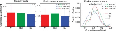
Mean (+SD) correlation coefficient between acoustic energy within MC and ES stimuli and firing rate, quantifying the ability of units in areas A1, CM, and CL to follow temporal structure of the stimuli. P values shown in parentheses were obtained from Kolmogorov-Smirnov tests. Left and center: mean + SD. Right: same data as in center displayed as distributions constructed by binning the entire data range into 1,000 bins and smoothing with a Gaussian kernel (σ = 10 bins).

A practical outcome of this study should be identification of neural parameters that would allow distinguishing CM from CL in future studies based on response properties only. Figure 10 shows maps of seven candidate parameters that were selected on the basis of significant differences between CM and CL (maps smoothed with 2D Gaussian kernel, σ = 0.75 mm). Latency, and also elevation PI and linear discriminator bin width, arguably differentiated most reliably between the two caudal areas; however, there was still considerable variability between parameters and animals.

In an attempt to improve CM/CL identification, we applied PCA to the same parameters. The first PC (PC1) explained a modest amount of variance (38%; Fig. 11A). However, the pattern of correlation of PC1 with the original neural parameters demonstrated that it had captured these facets of the parameters that were associated with the CM vs. CL difference. Namely, PC1 was moderately positively correlated with the parameters that were lower in CM than in CL (latency and linear discriminator best bandwidth) and moderately negatively correlated with those that were lower in CL than in CM (correlation of firing rate with acoustic structure and spatial PI; Fig. 11B). Maps of PC1 show that this compound parameter might be used to distinguish between CM and CL with reasonable accuracy (Fig. 11C).

DISCUSSION

Caudal belt vs. core.

Frequency tuning was wider in the caudal belt than in the core (Fig. 3), indicating spectral integration previously demonstrated physiologically in the lateral (Rauschecker et al. 1995; Rauschecker and Tian 2004) and medial (Kuśmierek and Rauschecker 2009) belt and with fMRI in monkeys and humans (e.g., Chevillet et al. 2011; Petkov et al. 2006; Wessinger et al. 2001). Similarly, the higher number of peaks in the frequency-PFR curves compared with A1 suggests integration across frequency ranges (Fig. 3, cf. Rauschecker et al. 1997). Still, cochleotopy was found in areas CL and CM. Although CM is commonly assumed to be cochleotopic, we believe that ours is actually the first electrophysiological demonstration of cochleotopic organization in CM proper (i.e., separately from CL) of the rhesus monkey. Because of shifting nomenclature, earlier reports of cochleotopy in CM might have been from CM or CL (Merzenich and Brugge 1973).

Another remarkable difference between A1 and caudal belt was the lack of correlation between unit latency and BF (Fig. 7, right). We and others have shown that A1 neurons tuned to low frequencies respond with longer latencies than those tuned to high frequencies (Kuśmierek and Rauschecker 2009; Lakatos et al. 2005; Scott et al. 2011; see also Mendelson et al. 1997 in the cat and Bendor and Wang 2008 in the marmoset). Beyond A1, such correlation between BF and latency in areas R, RM, and MM has been shown by us (Kuśmierek and Rauschecker 2009) and in area R of the marmoset by Bendor and Wang (2008). Scott et al. (2011), on the other hand, did not find a significant correlation between BF and latency in macaque area R. In the caudal belt, a lack of correlation between BF and latency has been found in rhesus CM and CL (this report) and in marmoset CM (Kajikawa et al. 2005). Previously we proposed that a subcortical mechanism extracting frequency based on temporal information might be responsible for the existence of the correlation (Kuśmierek and Rauschecker 2009). The present result suggests that this mechanism would be absent in the pathways reaching the caudal belt.

CM vs. CL: stimulus selectivity.

CL consistently showed low stimulus selectivity as measured with PI and linear discriminator analysis. It is noteworthy that selectivity in CM was higher than in CL and matched that in A1 (P = 0.97) when measured with linear discriminator performance (which is sensitive to temporal structure of response) in ES, whose temporal structure is pronounced and important for processing (Gygi et al. 2004; Kuśmierek and Rauschecker 2009; Warren and Verbrugge 1984). This suggests that CM is particularly well suited to process temporal information (see Temporal factors below).

Classification accuracy based on population response was similar in all areas, with a small advantage for CL (Fig. 5, Kuśmierek et al. 2012). This result was somewhat unexpected, as it implies an increase of categorical “what” information in CL compared with A1. MC-selective neurons have been shown in CL before (Tian et al. 2001), but their number was relatively small. Similarly, the effect here was minute compared with the high classification accuracy found previously in anterior areas (Kuśmierek et al. 2012).

In summary, of the two caudal belt areas CM is better suited for stimulus representation, with emphasis on the temporal structure of stimuli.

Spatial selectivity.

Higher azimuth selectivity in CL than in CM is demonstrated here with PI, most reliably when tested with WN. When tested with PT and BPN, the difference was significant in some variants of the analysis and close to significance in others (see Table 1). This result complements less direct measures employed previously by others (Miller and Recanzone 2009; Woods et al. 2006). Importantly, we extend the finding to the elevation domain. Earlier studies measuring elevation tuning in monkey auditory cortex did not distinguish between CM and CL (Recanzone et al. 2000a; Zhou and Wang 2012).

CL exhibited increased elevation selectivity only for wideband stimuli, reflecting psychophysical constraints of localization in the vertical plane, which depends on stimulus bandwidth in humans and monkeys (e.g., Brown et al. 1982; Recanzone et al. 2000a; Roffler and Butler 1968). For localization in azimuth, we found no dependence of spatial selectivity on bandwidth, contrary to psychophysical data (Brown et al. 1980; Recanzone et al. 2000a). However, psychophysical azimuth localization thresholds even for narrowest-band stimuli were far lower than the 45° azimuth step used in our study (Brown et al. 1982; Recanzone et al. 2000a). Elevation localization thresholds, on the other hand, were immeasurable for PT and comparable to our 30° elevation step for 1-octave BPN (Recanzone et al. 2000a).

In summary, CL is specialized for representing information about at least two-dimensional spatial location of sound stimuli (the dimension of distance was not studied), while CM does not differ from A1 in this respect. Thus increased spatial selectivity predicted by the proposed role of the dorsal stream in sound localization is limited to the lateral component of the caudal belt.

Temporal factors.

We found a significant advantage of CM over CL in several measures related to the timing of neural responses. Response latencies were substantially shorter in CM than in CL or A1 (Fig. 7, left). This indicates that CM receives auditory information not only from A1 (Rauschecker et al. 1997) but also from another, faster source, likely the antero-dorsal nucleus of the medial geniculate body (MGB; Bartlett and Wang 2011; Camalier et al. 2012; Hackett et al. 2007).

Latencies in CL are indistinguishable from those in A1 (Fig. 7, left; P > 0.7). While this does not preclude that CL receives the majority of its input from A1 (see Rauschecker et al. 1997; area “CM” in that study may have included CL), other sources likely contribute to CL activity as well. As discussed above, latencies are negatively correlated with BF in A1, but there is no such correlation in CL; this suggests that the low-BF units of CL are unlikely to be driven by input from low-BF A1 neurons. One source of auditory input to CL could be the postero-dorsal nucleus of the MGB (Bartlett and Wang 2011; Hackett et al. 2007).

Rauschecker et al. (1997) demonstrated that CM (or caudal belt) is on a hierarchically higher level than A1, which may appear to contradict our finding that latencies in CM are shorter than in A1 and latencies in CL are similar to A1. It is noteworthy, however, that a lesion to A1 markedly reduced responses to tones in CM/caudal belt but responses to complex sounds were still present (Rauschecker et al. 1997), consistent with a source other than A1 (presumably, the antero- and postero-dorsal MGB nuclei) driving the area. This source would be responsible for short-latency CM and CL responses, while A1-driven responses may have longer latencies. The fact that Rauschecker et al. (1997) recorded from anesthetized animals may have also affected the response properties (whether latency or tuning for tones vs. complex sounds).

Taken together, analyses of response latencies highlight the importance of thalamic inputs to the caudal auditory belt that are parallel to the classic serial route via the ventral nucleus of MGB, A1, and intracortical connections (Hackett et al. 1998; Kaas and Hackett 2000). Whether this means that auditory processing streams are segregated already on subcortical levels remains to be determined, but this possibility has been raised previously (Rauschecker et al. 1997; Rauschecker and Tian 2000).

In addition to short response latencies, other temporal measures distinguish CM from CL. First, the linear discriminator performance depends on neurons producing repeatable spiking patterns to stimuli; the temporal accuracy with which they are repeated is captured by the discriminator's best bin width. Second, we have demonstrated previously that in the core and medial belt spiking patterns often follow spectrotemporal features of stimuli (Kuśmierek and Rauschecker 2009). In the present study, we directly measured correlation of spiking patterns with the course of spectrotemporal change. Both measures yielded similar results: temporal accuracy was higher in CM than in CL, with A1 showing typically intermediate values (Fig. 8 and Fig. 9). Further studies of caudal belt temporal properties may be needed, as (in anesthetized monkeys) more A1 than CM neurons synchronized to high click frequencies (Oshurkova et al. 2008), while Scott et al. (2011) found no significant difference with a tendency for a higher synchronization limit in CM.

Our results show that the gradient of latencies and temporal integration windows, which had been found previously to progress from area A1 to the rostral (R) and rostrotemporal (RT) areas in macaques and marmosets (Bendor and Wang 2008; Kuśmierek et al. 2009; Pfingst and O'Connor 1981; Recanzone et al. 2000b; Scott et al. 2011), extends in the caudal direction, but only to area CM and not to CL.

Distinguishing CM from CL.

Direct comparisons of response properties in CM vs. CL have been virtually lacking in the literature so far. Thus, when delineating the boundary between the two areas, we elected to rely on gross anatomy only and to establish differences in response properties in this study. These differences, apart from providing insight into auditory processing in the caudal belt, may be used in future studies to determine the location of the CM/CL boundary solely on the basis of physiology. However, most neural properties overlapped to a large extent between areas, even if they were statistically different. Consequently, mapping these properties to the recording area usually did not yield a clear-cut boundary (Fig. 10), with response latencies probably providing the clearest differentiation. Thus, unless a single property clearly distinguishing CM from CL is found in a future study, combining several properties by PCA or other means might be the optimal solution in the absence of histological data (Fig. 11).

Organization of dorsal stream.

The traditional model of the auditory dorsal stream emphasizes its role in processing spatial information (Rauschecker 1998; Rauschecker and Tian 2000; Recanzone 2000), which is supported by many studies in monkeys and humans (Deouell et al. 2007; Miller and Recanzone 2009; Warren et al. 2002; Zimmer and Macaluso 2005). Nonspatial functions have been mapped to the dorsal stream as well (Belin and Zatorre 2000; Dhanjal et al. 2008; Geschwind 1965; Hickok et al. 2009; Leaver et al. 2009; Lewis et al. 2005; Perry et al. 1999; Rauschecker 2011; Rauschecker and Scott 2009; Wernicke 1874; Wise et al. 2001), especially in its extension to premotor and prefrontal cortices (see also introduction). This raises the possibility of a division of labor within the dorsal stream, with different subregions or substreams performing different functions. The caudal belt areas are assumed to be the earliest stage of the dorsal stream (Hackett 2011; Kaas and Hackett 2000), and indeed they have direct (Lewis and Van Essen 2000; Romanski et al. 1999a, 1999b; Ward et al. 1946; Yeterian et al. 2012) and indirect (Smiley et al. 2007) connections with parietal, premotor, or dorsal prefrontal cortices. We found temporally precise responses bound to acoustic structure and pronounced spatial selectivity in the caudal belt in the same monkeys. However, these properties were segregated, the latter being more apparent in CL and the former more apparent in CM—again an indication of possible division of labor within the dorsal stream.

This segregation is consistent with other electrophysiological and anatomical data. Higher spatial selectivity in CL than in CM has been shown previously for azimuth only (Miller and Recanzone 2009; Woods et al. 2006). Camalier et al. (2012) demonstrated particularly fast latencies in CM. A region representing spatial location of sounds is expected to be strongly linked to the visual system in order to relate sounds to visual objects in space; indeed, visual connections and projections from area 7a (which is involved in coding location of targets for reaching; Andersen 1997) are stronger in CL than in CM (Falchier et al. 2010; Smiley et al. 2007).

The existence of more than two processing streams in the auditory cortical system has been proposed previously (Belin and Zatorre 2000; Kaas and Hackett 1999; Schubotz et al. 2003). The segregation of spatial and temporal tuning between CL and CM in the dorsal auditory stream may suggest the existence of functional substreams within this processing pathway. It remains to be determined whether this segregation continues beyond the earliest part of the dorsal stream and therefore warrants distinguishing separate substreams. Somatosensory projections targeting medial and lateral caudal belt alike (Smiley et al. 2007), as well as modulation of responses in areas of the intraparietal sulcus by both spatial and audio-motor aspects of sounds (Gifford and Cohen 2005; Schlack et al. 2005), suggest that despite some degree of specialization the dorsal stream should still be considered a single functional entity.

The role of a fast and temporally precise representation of sounds in dorsal stream functions, whether spatial or nonspatial, will also need further elucidation. Some authors have proposed that fast latencies may be beneficial for quick action selection performed by the dorsal stream, possibly under a threat (Camalier et al. 2012; Jääskeläinen et al. 2004). Alternatively, fast response latency may serve by producing an “initial guess” of object identity in the dorsal stream, subsequently utilized by the ventral stream for slower and more specific analysis, or by attentional mechanisms (Ahveninen et al. 2006). A similar explanation has been proposed for faster latencies in the dorsal than in the ventral stream of the visual cortex (Schroeder et al. 1998).

GRANTS

This work was supported by National Institute of Neurological Disorders and Stroke Grants R01-NS-052494 and R56-NS-052494-06A1 to J. P. Rauschecker.

DISCLOSURES

No conflicts of interest, financial or otherwise, are declared by the author(s).

AUTHOR CONTRIBUTIONS

Author contributions: P.K. and J.P.R. conception and design of research; P.K. analyzed data; P.K. and J.P.R. interpreted results of experiments; P.K. prepared figures; P.K. drafted manuscript; P.K. and J.P.R. edited and revised manuscript; P.K. and J.P.R. approved final version of manuscript.

REFERENCES

- Ahveninen J, Jääskeläinen IP, Raij T, Bonmassar G, Devore S, Hämäläinen M, Levänen S, Lin FH, Sams M, Shinn-Cunningham BG, Witzel T, Belliveau JW. Task-modulated “what” and “where” pathways in human auditory cortex. Proc Natl Acad Sci USA 103: 14608–14613, 2006 [DOI] [PMC free article] [PubMed] [Google Scholar]
- Andersen RA. Multimodal integration for the representation of space in the posterior parietal cortex. Philos Trans R Soc Lond B Biol Sci 352: 1421–1428, 1997 [DOI] [PMC free article] [PubMed] [Google Scholar]
- Arnott SR, Binns MA, Grady CL, Alain C. Assessing the auditory dual pathway model in humans. Neuroimage 22: 401–408, 2004 [DOI] [PubMed] [Google Scholar]
- Bartlett EL, Wang X. Correlation of neural response properties with auditory thalamus subdivisions in the awake marmoset. J Neurophysiol 105: 2647–2667, 2011 [DOI] [PMC free article] [PubMed] [Google Scholar]
- Belin P, Zatorre RJ. “What”, “where” and “how” in auditory cortex. Nat Neurosci 3: 965–966, 2000 [DOI] [PubMed] [Google Scholar]
- Bendor D, Wang X. Neural response properties of primary, rostral, and rostrotemporal core fields in the auditory cortex of marmoset monkeys. J Neurophysiol 100: 888–906, 2008 [DOI] [PMC free article] [PubMed] [Google Scholar]
- Brown CH, Beecher MD, Moody DB, Stebbins WC. Localization of noise bands by Old World monkeys. J Acoust Soc Am 68: 127–132, 1980 [DOI] [PubMed] [Google Scholar]
- Brown CH, Schessler T, Moody D, Stebbins W. Vertical and horizontal sound localization in primates. J Acoust Soc Am 72: 1804–1811, 1982 [DOI] [PubMed] [Google Scholar]
- Camalier CR, D'Angelo WR, Sterbing-D'Angelo SJ, de la Mothe LA, Hackett TA. Neural latencies across auditory cortex of macaque support a dorsal stream supramodal timing advantage in primates. Proc Natl Acad Sci USA 109: 18168–18173, 2012 [DOI] [PMC free article] [PubMed] [Google Scholar]
- Chevillet M, Riesenhuber M, Rauschecker JP. Functional correlates of the anterolateral processing hierarchy in human auditory cortex. J Neurosci 31: 9345–9352, 2011 [DOI] [PMC free article] [PubMed] [Google Scholar]
- Deouell LY, Heller AS, Malach R, D'Esposito M, Knight RT. Cerebral responses to change in spatial location of unattended sounds. Neuron 55: 985–996, 2007 [DOI] [PubMed] [Google Scholar]
- DeWitt I, Rauschecker JP. Phoneme and word recognition in the auditory ventral stream. Proc Natl Acad Sci USA 109: 505–514, 2012 [DOI] [PMC free article] [PubMed] [Google Scholar]
- Dhanjal NS, Handunnetthi L, Patel MC, Wise RJ. Perceptual systems controlling speech production. J Neurosci 28: 9969–9975, 2008 [DOI] [PMC free article] [PubMed] [Google Scholar]
- Falchier A, Schroeder CE, Hackett TA, Lakatos P, Nascimento-Silva S, Ulbert I, Karmos G, Smiley JF. Projection from visual areas V2 and prostriata to caudal auditory cortex in the monkey. Cereb Cortex 20: 1529–1538, 2010 [DOI] [PMC free article] [PubMed] [Google Scholar]
- Geschwind N. Disconnexion syndromes in animals and man. Brain 88: 237–294, 585–644, 1965 [DOI] [PubMed] [Google Scholar]
- Gifford GW, 3rd, Cohen YE. Spatial and non-spatial auditory processing in the lateral intraparietal sulcus. Exp Brain Res 162: 509–512, 2005 [DOI] [PubMed] [Google Scholar]
- Goodale MA, Milner A. Separate visual pathways for perception and action. Trends Neurosci 15: 20–25, 1992 [DOI] [PubMed] [Google Scholar]
- Gygi B, Kidd GR, Watson C. Spectral-temporal factors in the identifications of environmental sounds. J Acoust Soc Am 116: 1252–1265, 2004 [DOI] [PubMed] [Google Scholar]
- Hackett TA. Information flow in the auditory cortical network. Hear Res 271: 133–146, 2011 [DOI] [PMC free article] [PubMed] [Google Scholar]
- Hackett TA, de la Mothe LA, Ulbert I, Karmos G, Smiley J, Schroeder CE. Multisensory convergence in auditory cortex. II. Thalamocortical connections of the caudal superior temporal plane. J Comp Neurol 502: 924–952, 2007 [DOI] [PubMed] [Google Scholar]
- Hackett TA, Stepniewska I, Kaas JH. Subdivisions of auditory cortex and ipsilateral cortical connections of the parabelt auditory cortex in macaque monkeys. J Comp Neurol 394: 475–495, 1998 [DOI] [PubMed] [Google Scholar]
- Hauser MD. Functional referents and acoustic similarity: field playback experiments with rhesus monkeys. Anim Behav 55: 1647–1658, 1998 [DOI] [PubMed] [Google Scholar]
- Hickok G, Okada K, Serences JT. Area Spt in the human planum temporale supports sensory-motor integration for speech processing. J Neurophysiol 101: 2725–2732, 2009 [DOI] [PubMed] [Google Scholar]
- Jääskeläinen IP, Ahveninen J, Bonmassar G, Dale AM, Ilmoniemi RJ, Levänen S, Lin FH, May P, Melcher J, Stufflebeam S, Tiitinen H, Belliveau JW. Human posterior auditory cortex gates novel sounds to consciousness. Proc Natl Acad Sci USA 101: 6809–6814, 2004 [DOI] [PMC free article] [PubMed] [Google Scholar]
- Jackson LL, Heffner RS, Heffner HE. Free-field audiogram of the Japanese macaque (Macaca fuscata). J Acoust Soc Am 106: 3017–3023, 1999 [DOI] [PubMed] [Google Scholar]
- Kaas JH, Hackett TA. “What” and “where” processing in auditory cortex. Nat Neurosci 2: 1045–1047, 1999 [DOI] [PubMed] [Google Scholar]
- Kaas JH, Hackett TA. Subdivisions of auditory cortex and processing streams in primates. Proc Natl Acad Sci USA 97: 11793–11799, 2000 [DOI] [PMC free article] [PubMed] [Google Scholar]
- Kajikawa Y, de la Mothe L, Blumell S, Hackett TA. A comparison of neuron response properties in areas A1 and CM of the marmoset monkey auditory cortex: tones and broadband noise. J Neurophysiol 93: 22–34, 2005 [DOI] [PubMed] [Google Scholar]
- Kravitz DJ, Saleem KS, Baker CI, Mishkin M. A new neural framework for visuospatial processing. Nat Rev Neurosci 12: 217–230, 2011 [DOI] [PMC free article] [PubMed] [Google Scholar]
- Krumbholz K, Schönwiesner M, von Cramon DY, Rübsamen R, Shah NJ, Zilles K, Fink GR. Representation of interaural temporal information from left and right auditory space in the human planum temporale and inferior parietal lobe. Cereb Cortex 15: 317–324, 2005a [DOI] [PubMed] [Google Scholar]
- Krumbholz K, Schönwiesner M, Rübsamen R, Zilles K, Fink GR, von Cramon DY. Hierarchical processing of sound location and motion in the human brainstem and planum temporale. Eur J Neurosci 21: 230–238, 2005b [DOI] [PubMed] [Google Scholar]
- Kuśmierek P, Ortiz M, Rauschecker JP. Sound-identity processing in early areas of the auditory ventral stream in the macaque. J Neurophysiol 107: 1123–1141, 2012 [DOI] [PMC free article] [PubMed] [Google Scholar]
- Kuśmierek P, Rauschecker JP. Functional specialization of medial auditory belt cortex in the alert rhesus monkey. J Neurophysiol 102: 1606–1622, 2009 [DOI] [PMC free article] [PubMed] [Google Scholar]
- Lakatos P, Pincze Z, Fu KM, Javitt DC, Karmos G, Schroeder CE. Timing of pure tone and noise-evoked responses in macaque auditory cortex. Neuroreport 16: 933–937, 2005 [DOI] [PubMed] [Google Scholar]
- Leaver A, Van Lare JE, Zielinski BA, Halpern A, Rauschecker JP. Brain activation during anticipation of sound sequences. J Neurosci 29: 2477–2485, 2009 [DOI] [PMC free article] [PubMed] [Google Scholar]
- Lewis JW, Brefczynski JA, Phinney RE, Janik JJ, DeYoe EA. Distinct cortical pathways for processing tool versus animal sounds. J Neurosci 25: 5148–5158, 2005 [DOI] [PMC free article] [PubMed] [Google Scholar]
- Lewis JW, Van Essen ED. Corticocortical connections of visual, sensorimotor, and multimodal processing areas in the parietal lobe of the macaque monkey. J Comp Neurol 428: 112–137, 2000 [DOI] [PubMed] [Google Scholar]
- Maeder PP, Meuli RA, Adriani M, Bellmann A, Fornari E, Thiran JP, Pittet A, Clarke S. Distinct pathways involved in sound recognition and localization: a human fMRI study. Neuroimage 14: 802–816, 2001 [DOI] [PubMed] [Google Scholar]
- McLaren DG, Kosmatka KJ, Oakes TR, Kroenke CD, Kohama SG, Matochik JA, Ingram DK, Johnson SC. A population-average MRI-based atlas collection of the rhesus macaque. Neuroimage 45: 52–59, 2009 [DOI] [PMC free article] [PubMed] [Google Scholar]
- Mendelson JR, Schreiner CE, Sutter ML. Functional topography of cat primary auditory cortex: response latencies. J Comp Physiol A 181: 615–633, 1997 [DOI] [PubMed] [Google Scholar]
- Merzenich MM, Brugge JF. Representation of the cochlear partition on the superior temporal plane of the macaque monkey. Brain Res 50: 275–296, 1973 [DOI] [PubMed] [Google Scholar]
- Miller LM, Recanzone GH. Populations of auditory cortical neurons can accurately encode acoustic space across stimulus intensity. Proc Natl Acad Sci USA 106: 5931–5935, 2009 [DOI] [PMC free article] [PubMed] [Google Scholar]
- Mishkin M, Ungerleider LG, Macko KA. Object vision and spatial vision: two cortical pathways. Trends Neurosci 6: 414–417, 1983 [Google Scholar]
- Morecraft RJ, Stilwell-Morecraft KS, Cipolloni PB, Ge J, McNeal DW, Pandya DN. Cytoarchitecture and cortical connections of the anterior cingulate and adjacent somatomotor fields in the rhesus monkey. Brain Res Bull 87: 457–397, 2012 [DOI] [PMC free article] [PubMed] [Google Scholar]
- Oshurkova E, Scheich H, Brosch M. Click train encoding in primary and non-primary auditory cortex of anesthetized macaque monkeys. Neuroscience 153: 1289–1299, 2008 [DOI] [PubMed] [Google Scholar]
- Perry DW, Zatorre RJ, Petrides M, Alivisatos B, Meyer E, Evans AC. Localization of cerebral activity during simple singing. Neuroreport 10: 3979–3984, 1999 [DOI] [PubMed] [Google Scholar]
- Petkov CI, Kayser C, Augath M, Logothetis NK. Functional imaging reveals numerous fields in the monkey auditory cortex. PLoS Biol 4: 1213–1226, 2006 [DOI] [PMC free article] [PubMed] [Google Scholar]
- Pfingst BE, O'Connor TA. Characteristics of neurons in auditory cortex of monkeys performing a simple auditory task. J Neurophysiol 45: 16–34, 1981 [DOI] [PubMed] [Google Scholar]
- Rauschecker JP. Processing of complex sounds in the auditory cortex of cat, monkey and man. Acta Otolaryngol (Stockh) 532: 34–38, 1997 [DOI] [PubMed] [Google Scholar]
- Rauschecker JP. Parallel processing in the auditory cortex of primates. Audiol Neurootol 3: 86–103, 1998 [DOI] [PubMed] [Google Scholar]
- Rauschecker JP. Cortical processing of auditory space: pathways and plasticity. In: Spatial Processing in Navigation, Imagery, and Perception. edited by Mast FJ̈, ancke L. New York: Springer-Verlag, 2007, p. 389–410 [Google Scholar]
- Rauschecker JP. An expanded role for the dorsal auditory pathway in sensorimotor control and integration. Hear Res 271: 16–25, 2011 [DOI] [PMC free article] [PubMed] [Google Scholar]
- Rauschecker JP. Ventral and dorsal streams in the evolution of speech and language. Front Evol Neurosci 4: 7, 2012 [DOI] [PMC free article] [PubMed] [Google Scholar]
- Rauschecker JP, Scott SK. Maps and streams in the auditory cortex: nonhuman primates illuminate human speech processing. Nat Neurosci 12: 718–724, 2009 [DOI] [PMC free article] [PubMed] [Google Scholar]
- Rauschecker JP, Tian B. Mechanisms and streams for processing of “what” and “where” in auditory cortex. Proc Natl Acad Sci USA 97: 11800–11806, 2000 [DOI] [PMC free article] [PubMed] [Google Scholar]
- Rauschecker JP, Tian B. Processing of band-passed noise in the lateral auditory belt cortex of the rhesus monkey. J Neurophysiol 91: 2578–2589, 2004 [DOI] [PubMed] [Google Scholar]
- Rauschecker JP, Tian B, Hauser M. Processing of complex sounds in the macaque nonprimary auditory cortex. Science 268: 111–114, 1995 [DOI] [PubMed] [Google Scholar]
- Rauschecker JP, Tian B, Pons T, Mishkin M. Serial and parallel processing in rhesus monkey auditory cortex. J Comp Neurol 382: 89–103, 1997 [PubMed] [Google Scholar]
- Recanzone GH. Spatial processing in the auditory cortex of the macaque monkey. Proc Natl Acad Sci USA 97: 11829–11835, 2000 [DOI] [PMC free article] [PubMed] [Google Scholar]
- Recanzone GH. Representation of con-specific vocalizations in the core and belt areas of the auditory cortex in the alert macaque monkey. J Neurosci 28: 13184–13193, 2008 [DOI] [PMC free article] [PubMed] [Google Scholar]
- Recanzone GH, Guard DC, Phan ML, Su TK. Correlation between the activity of single auditory cortical neurons and sound-localization behavior in the macaque monkey. J Neurophysiol 83: 2723–2739, 2000a [DOI] [PubMed] [Google Scholar]
- Recanzone GH, Guard DC, Phan ML. Frequency and intensity response properties of single neurons in the auditory cortex of the behaving macaque monkey. J Neurophysiol 83: 2315–2331, 2000b [DOI] [PubMed] [Google Scholar]
- Roffler SK, Butler RA. Factors that influence the localization of sound in the vertical plane. J Acoust Soc Am 43: 1255–1259, 1968 [DOI] [PubMed] [Google Scholar]
- Romanski LM, Tian B, Fritz J, Mishkin M, Goldman-Rakic PS, Rauschecker JP. Dual streams of auditory afferents target multiple domains in the primate prefrontal cortex. Nat Neurosci 2: 1131–1136, 1999a [DOI] [PMC free article] [PubMed] [Google Scholar]
- Romanski LM, Bates JF, Goldman-Rakic PS. Auditory belt and parabelt projections to the prefrontal cortex in the rhesus monkey. J Comp Neurol 403: 141–157, 1999b [DOI] [PubMed] [Google Scholar]
- Russ BE, Ackelson AL, Baker AE, Cohen YE. Coding of auditory-stimulus identity in the auditory non-spatial processing stream. J Neurophysiol 99: 87–95, 2008 [DOI] [PMC free article] [PubMed] [Google Scholar]
- Saleem K, Logothetis N. A Combined MRI and Histology Atlas of the Rhesus Monkey Brain in Stereotaxic Coordinates. San Diego, CA: Academic, 2007 [Google Scholar]
- Schlack A, Sterbing-D'Angelo SJ, Hartung K, Hoffmann KP, Bremmer F. Multisensory space representations in the macaque ventral intraparietal area. J Neurosci 25: 4616–4625, 2005 [DOI] [PMC free article] [PubMed] [Google Scholar]
- Schroeder CE, Mehta AD, Givre SJ. A spatiotemporal profile of visual system activation revealed by current source density analysis in the awake macaque. Cereb Cortex 8: 575–592, 1998 [DOI] [PubMed] [Google Scholar]
- Schubotz RI, von Cramon DY, Lohmann G. Auditory what, where, and when: a sensory somatotopy in lateral premotor cortex. Neuroimage 20: 173–185, 2003 [DOI] [PubMed] [Google Scholar]
- Scott BH, Malone BJ, Semple MN. Transformation of temporal processing across auditory cortex of awake macaques. J Neurophysiol 10: 712–730, 2011 [DOI] [PMC free article] [PubMed] [Google Scholar]
- Smiley JF, Hackett TA, Ulbert I, Karmas G, Lakatos P, Javitt DC, Schroeder CE. Multisensory convergence in auditory cortex. I. Cortical connections of the caudal superior temporal plane in macaque monkeys. J Comp Neurol 502: 894–923, 2007 [DOI] [PubMed] [Google Scholar]
- Tian B, Reser D, Durham A, Kustov A, Rauschecker JP. Functional specialization in rhesus monkey auditory cortex. Science 292: 290–293, 2001 [DOI] [PubMed] [Google Scholar]
- Ungerleider LG, Mishkin M. Two cortical visual systems. In: Analysis of Visual Behaviour, edited by Ingle DJ, Goodale MA, Mansfield RJ. Cambridge, MA: MIT Press, 1982, p. 549–586 [Google Scholar]
- Ward AA, Jr, Peden JK, Sugar O. Cortico-cortical connections in the monkey with special reference to area 6. J Neurophysiol 9: 453–461, 1946 [DOI] [PubMed] [Google Scholar]
- Warren JD, Zielinski BA, Green GG, Rauschecker JP, Griffiths TD. Analysis of sound source motion by the human brain. Neuron 34: 1–20, 2002 [DOI] [PubMed] [Google Scholar]
- Warren WH, Verbrugge RR. Auditory perception of breaking and bouncing events: a case study in ecological acoustics. J Exp Psychol Hum Percept Perform 10: 704–712, 1984 [DOI] [PubMed] [Google Scholar]
- Wernicke C. Der aphasische Symptomenkomplex: Eine psychologische Studie auf anatomischer Basis. Breslau, Germany: Cohn and Weigert, 1874 [Google Scholar]
- Wessinger CM, VanMeter J, Tian B, Van Lare J, Pekar J, Rauschecker JP. Hierarchical organization of the human auditory cortex revealed by functional magnetic resonance imaging. J Cogn Neurosci 13: 1–7, 2001 [DOI] [PubMed] [Google Scholar]
- Wise RJ, Scott SK, Blank SC, Mummery CJ, Murphy K, Warburton EA. Separate neural subsystems within “Wernicke's area.” Brain 124: 83–95, 2001 [DOI] [PubMed] [Google Scholar]
- Woods TM, Lopez SE, Long JH, Rahman JE, Recanzone GH. Effects of stimulus azimuth and intensity on the single-neuron activity in the auditory cortex of the alert macaque monkey. J Neurophysiol 96: 3323–3337, 2006 [DOI] [PubMed] [Google Scholar]
- Yeterian EH, Pandya DN, Tomaiuolo F, Petrides M. The cortical connectivity of the prefrontal cortex in the monkey brain. Cortex 48: 58–81, 2012 [DOI] [PMC free article] [PubMed] [Google Scholar]
- Zhou Y, Wang X. Level dependence of spatial processing in primate auditory cortex. J Neurophysiol 108: 810–826, 2012 [DOI] [PMC free article] [PubMed] [Google Scholar]
- Zimmer U, Macaluso E. High binaural coherence determines successful sound localization and increased activity in posterior auditory areas. Neuron 47: 893–905, 2005 [DOI] [PubMed] [Google Scholar]