Haplotype Information and Linkage Disequilibrium Mapping for Single Nucleotide Polymorphisms

Abstract

Single nucleotide polymorphisms in the human genome have become an increasingly popular topic in that their analyses promise to be a key step toward personalized medicine. We investigate two related questions, how much the haplotype information contributes to linkage disequilibrium (LD) mapping and whether an in silico haplotype construction preceding the LD analysis can help. For disease gene mapping, using both simulated and real data sets on cystic fibrosis and the Alzheimer disease, we reached the following conclusions: (1) for simple Mendelian diseases, in which case a tractable full statistical model can be developed, the loss of haplotype information for either control or disease data do not have a great impact on LD fine mapping, and haplotype inference should be carried out jointly with LD mapping; (2) for complex diseases, inferring haplotype phases for individuals prior to LD mapping helps achieve a better accuracy. An improved version of the linkage disequilibrium mapping program, BLADE v2, is available at http://www.fas.harvard.edu/junliu/TechRept/03folder/bladev2.tgz.

Available data on tightly linked single nucleotide polymorphisms (SNPs) are experiencing a dramatic growth. Because it is commonly believed that haplotypes are essential for disease-gene discovery, genetic demography, and chromosomal evolution studies, as well as linkage disequilibrium (LD) mappings (Fallin and Schork 2000; Fallin et al. 2001), much effort has been made in phasing individuals' two haplotypes, either experimentally or computationally. When the family-based genetic information is available, it is relatively easy to infer the individuals' phases from their genotype data, although there are still ambiguities (Hodge et al. 1999; Hoh and Hodge 2000). In population-based case-control studies, the experimental ascertainment of individuals' haplotypes requires laborious and cost-prohibitive chromosomal isolation and other molecular-haplotyping strategies (Clark et al. 2001). Alternatively, one may explore in silico methods for inferring haplotypes from a sample of genotyped, but unphased diploid individuals (Clark 1990; Excoffier and Slatkin 1995; Hawley and Kidd 1995; Long et al. 1995; Chiano and Clayton 1998; Stephens et al. 2001; Niu et al. 2002; Qin et al. 2002).

Although the available in silico haplotyping methods are cost-effective and have shown considerable power, they are still error-prone (Fallin and Schork 2000; Clark et al. 2001), and such errors may mislead the subsequent LD analysis. To deepen this feeling of discomfort, we note that the genotyping errors have been shown to seriously affect several pairwise LD measures (Akey et al. 2001). Ifthe goal of the SNP analysis is to estimate the location of the disease-related mutation relative to a set of tightly linked markers, it is of interest to assess how much the haplotype information helps improve the accuracy. Obviously, there is no difference at all if only a single-marker-based method is used.

Realizing that the single- or pair-marker methods are unable to fully exploit the information of the closely linked markers, researchers have been interested in truly haplotype-based multi-marker LD fine-mapping methods for case-control genetic marker data (McPeek and Strahs 1999; Liu et al. 2001; Morris et al. 2002). In particular, the model in Liu et al. (2001) assumes that the disease haplotypes can be grouped into k+1 clusters, corresponding to k distinct founder chromosomes and a null cluster for all other disease chromosomes without a founder mutation. Each of the k non-null clusters is characterized by an ancestral haplotype associated with a disease-causing mutation coalescing to a single time point (age). These k ancestral mutations are assumed to occur at the same (or nearly the same) location. Through a Bayesian approach, the resulting algorithm BLADE can handle complications such as missing marker data, multiple founders, and the presence of unphased chromosomes (Liu et al. 2001). Although BLADE is designed mainly to deal with simple Mendelian disorders, we demonstrate that it can also be applied to locate the disease-related mutation(s) for complex diseases such as the Alzheimer disease (AD). A main reason for this is that the null cluster can accommodate those case haplotypes that do not contain the mutation(s) being mapped.

An interesting question is whether the explicit construction of the case or control haplotypes before the LD mapping is necessary for an efficient use of the available multi-marker information. Conceptually, haplotype inference and the location estimation can be achieved at the same time via a joint statistical model. Because the uncertainty in haplotype phasing is accounted for in this framework, the resulting location estimation can be more robust. To test this hypothesis, we conducted a permutation study of the cystic fibrosis (CF) data set (Kerem et al. 1989) and a study based on simulated genotype data sets of a hypothetical Mendelian disease. We show that ifthe inferred haplotypes are deemed as bona fide and being used subsequently for the location estimation, the untreated uncertainty in haplotype phasing is translated into a less-reliable result. It is thus desirable to modify the available in silico haplotyping methods to impute multiple compatible haplotype pairs for each unphased individual. On the other hand, a joint model may not be very meaningful in complex diseases, in which only a small fraction of the case haplotypes has the disease-causing mutations. We show that in a case-control study of the AD using high-density SNPs around a well-established susceptibility gene, apolipoprotein E (APOE), performing haplotype phasing prior to disease mutation mapping significantly improved the accuracy.

For high-density SNP markers, it is often inappropriate to treat SNPs on the control haplotypes as in linkage equilibrium, and an inhomogeneous Markov chain model appears appropriate when the markers are not too closely linked (Liu et al. 2001). Here, we describe an expectation-maximization (EM) algorithm to treat unphased control chromosomes under the Markov model. We tested the performance of BLADE under this circumstance and observed that the loss of control haplotype information does not have any material effect on the accuracy of the location estimate.

RESULTS

Throughout this section, we compared the following two strategies for fine mapping the disease mutation: (A) a direct analysis by jointly modeling haplotype uncertainty and LD for the unphased data, and (B) inferring the haplotypes first and then applying a fine-mapping algorithm to the ascertained haplotypes. Two LD mapping algorithms were used in this study, BLADE (Liu et al. 2001) and DHSMap (McPeek and Strahs 1999), both of which are capable of fine mapping on either phased or unphased disease data. While implementing strategy B, either HAPLOTYPER (Niu et al. 2002) or PLEM (Qin et al. 2002) was used to infer the haplotypes. Because BLADE can treat unphased control chromosomes under the Markov model, strategies A and B are also compared under two scenarios: (1) phased control haplotypes, and (2) unphased control genotypes. For DHSMap, comparison was made for scenario 1 only. Beside HAPLOTYPER and PLEM, we have also tested two other computational haplotyping methods, PHASE (Stephens et al. 2001) and Clark's (Clark 1990) method, for strategy B. The conclusions were similar to those using HAPLOTYPER and PLEM.

CF Data Set

The CF data set (Kerem et al. 1989) contains haplotypes on 23 bi-allelic markers around the CF transmembrane conductance regulator gene on chromosome 7q31.2. The control group has 92 haplotypes and the diseased group has 94. The founder mutation, ΔF₅₀₈, is located between markers 17 and 18, ∼0.88 cM away from the leftmost marker. By modeling the control haplotypes as an inhomogeneous Markov chain, BLADE gave a very accurate location estimate for the disease mutation. The posterior mean was 0.88 cM and the 95% probability interval (PI) for the location, which is defined as the central interval that contains 95% of the posterior probability mass, was [0.82, 0.93] cM (Liu et al. 2001).

To assess the impact of haplotype information of the disease chromosomes on LD mapping, we simulated 100 independent diseased group data sets. Each data set consists of 47 unphased diseased individuals with genotypes produced by random pairing of the 94 known disease haplotypes in the CF data set, effectively losing all of the haplotype information. Table 1 shows the comparisons between strategies A and B for fine-mapping the disease mutation (ΔF₅₀₈) for the 100 simulated data sets, using original control haplotypes. Two different LD mapping algorithms (BLADE and DHSMap), and four different haplotyping algorithms (i.e., HAPLOTYPER, PLEM, PHASE, and Clark's algorithm) were used to make this comparison. The results obtained by PLEM, PHASE, and Clark's algorithm are similar to that of HAPLOTYPER, and are omitted.

Table 1.

Comparison of Strategies A and B for Fine Mapping the Location of the Disease Mutation in 100 Data Sets Simulated Based on the Cystic Fibrosis Data

LD mapping algorithm	Strategy	Mean(pos)a	Std(pos)b	Mean 95% PI widthc	RMSEd	Overlape
BLADE	A	0.8600	0.0145	0.1461	0.0262	99%
	B	0.8647	0.0315	0.1402	0.0349	96%
DHSMap	A	0.8868	0.0428	0.2141	0.0432	96%
	B	0.9072	0.0702	0.1620	0.0749	66%

^aThe average of the 100 location estimates in the 100 simulations (true location = 0.88 cM).

^bThe sample standard deviation of the 100 location estimates.

^cThe average width of the 95% probability intervals (PIs) in the 100 simulations.

^dRoot mean square error (RMSE): square root of the average squared differences between the estimated and the true location, i.e., RMSE = 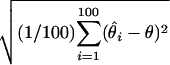, where θ is the true location and is the location estimate based on the i^th simulated data set.

^eThe percentage of times (in the 100 simulations) that the 95% PI overlapped with the target region.

To test the effect of losing control haplotype information, we generated another 100 independent “control group” data sets. In addition to randomly pairing up the disease haplotypes, we also randomly paired up the control haplotypes and estimated the Markov transition matrices from these unphased control genotypes by an EM algorithm (see Methods). The root mean square errors (RMSEs) of strategies A and B in this case, when BLADE was used as the LD mapping tool, were 0.0103 and 0.0339, respectively, leading to the same conclusion as shown in Table 1.

In summary, both strategies A and B were reasonably accurate in location estimations for this example, and the loss of control haplotype information did not seem to affect the estimation accuracy. Strategy A performed significantly better than strategy B in terms of both the RMSE of the disease location estimate and the percentage of times at which the 95% PI overlaps with the target region, regardless of the LD mapping method or haplotype phasing algorithm used in the analysis.

A Simulation for Simple Mendelian Disorders

To assess the robustness of the above findings, we simulated 100 populations of the disease haplotypes originating from a single founder 200 generations ago, assuming that there is a simple Mendelian disorder caused by a single founder mutation. We considered 20 bi-allelic markers, each 0.2 cM apart. The founder mutation was set to locate between markers 10 and 11, ∼1.9 cM away from the leftmost marker. The 200 disease haplotypes were given as 100 pairs of unphased genotypes, and the 200 control haplotypes were simulated from the equilibrium model. The same comparative study as for the CF data was performed, and the results are listed in Table 2.

Table 2.

Comparison of Strategies A and B for Fine Mapping the Founder Mutation Location in 100 Simulated Data Sets With a Hypothethical Mendelian Disorder

LD mapping algorithm	Strategya	Mean(pos)b	Std(pos)c	Mean 95% PI width	RMSEd	Overlape
BLADE	A	1.9042	0.0950	0.2194	0.0947	97%
	B	1.9064	0.1367	0.1721	0.1361	93%
DHSMap	A	1.9094	0.0881	0.1059	0.0882	86%
	B	1.9097	0.1292	0.0842	0.1289	70%

^aThe average of the 100 location estimates in the 100 simulations (true location = 0.88 cM).

^bThe sample standard deviation of the 100 location estimates.

^cThe average width of the 95% probability intervals (PIs) in the 100 simulations.

^dRoot mean square error (RMSE): square root of the average squared differences between the estimated and the true location, i.e., RMSE = , where θ is the ture location and is the location estimate based on the i^th simulated data set.

^eThe percentage of times (in the 100 simulations) that the 95% PI overlapped with the target region.

As a comparison, we also applied BLADE to the 100 sets of simulated disease haplotypes (i.e., the phase information is known). The average of the 100 location estimates was 1.90 cM with the RMSE of 0.095 cM, and 98 out of 100 times, the 95% PI overlapped with the target interval. This example again shows that strategy B is inferior to strategy A in both the RMSE of the location estimate and the percentage of times at which the 95% PI overlaps with the target region.

APOE SNP Data Set for AD

AD represents the most common type of dementia in the elderly (Rocchi et al. 2003). The human APOE gene, located on chromosome 19q13.2, encodes a single polypeptide chain with 299 amino acids, which is recognized as playing a major role in the transport of cholesterol and other lipids between peripheral tissues and the liver. There are three major isoforms, APOE-2, APOE-3, and APOE-4, differing from one another only by single amino acid substitutions. APOE-3 seems to be the normal isoform, and APOE-4 is shown to be an important AD-susceptible allele in the general population (for review, see Mahley and Rall Jr. 2000). The APOE SNP data set was published by Martin et al. (2000), containing 220 cases and 220 controls. Each multilocus genotype consists of marker data for 60 SNPs, spanning >3.5 Mb. In total, 9.4% of the SNP marker data were missing. Studies of APOE in primates and other mammals have suggested that APOE-4 is the ancestral allele in humans (Hanlon and Rubinsztein 1995; Gerdes and Cookson 1996), and therefore, it is expected that LD will extend over a short distance. Pairwise LD analysis by GOLD (Abecasis and Cookson 2000) also confirmed that LD extends only a small distance from the APOE-4 locus (data not shown).

From the original set of 60 SNPs, we used only those 30 SNPs in close proximity to the APOE-4 locus (Martin et al. 2000) to test the disease-mapping ability of BLADE, of which the SNPs were at least in moderate LD. The SNPs under consideration span a region of 615 kb. The APOE-4 (i.e., SNP528) is located 425 kb from the leftmost marker, SNP479. The physical distances were translated into genetic distances by assuming (1) a linear mapping function between the genetic distance (θ in cM) and the physical distance (x in Mb), when θ ≪ 1 M; and (2) 1 Mb = 1 cM. Although the conversion is known to be variable across the genome, comparison of chromosome 19 physical map versus the integrated genetic map shows that the approximation is reasonable for the region surrounding APOE (Martin et al. 2000). Because haplotyping algorithms cannot handle an excessively large portion of missing data, we deleted all of those genotypes that contained >30% missing marker data, or those with >5 consecutive missing markers. Therefore, 186 case and 189 control genotypes were actually used in this study.

By modeling the control haplotypes as a Markov chain and assuming k = 1 (i.e., a single founder mutation), we applied strategies A and B on the APOE data set. Because APOE-4 is the most susceptible SNP according to the single-marker LD measurement, we also tested on a modified data set with the APOE-4 marker removed from the original data set. In other words, we compared the performances of the two strategies solely on the basis of the genotype data of the remaining 29 SNPs.

The histograms of the posterior samples of the disease location θ obtained by the two strategies with APOE-4 deleted are shown in Figure 1. Alongside, we also displayed the single-marker LD measurements from the data set. The results are summarized in Table 3. We can see that both estimates are reasonably close to the true location, and both of the 95% PIs covered the true location (i.e., 0.425 cM). However, strategy B appears to have a significantly tighter 95% PI.

Figure 1.

Histograms of the posterior samples of the position parameter θ with APOE-4 deleted. (a) Results of strategy A; (b) results of strategy B. The origin of the x-axis is set to be the position of APOE-4, and the distal direction to be positive. The circles denote the single-marker LD measurements, and the triangle indicates that marker APOE-4 was deleted in our Bayesian analysis. The brackets denote the 95% PI bounds.

Table 3.

Comparison of Strategies A and B for Estimating the AD Locus From the APOE Data Set

Data Set	Strategy	Positiona	95% PI width	Size of cluster 1b
All 30 markers	A	0.4366	0.0283	82
	B	0.4272	0.0168	95
29 markers without APOE-4	A	0.4269	0.0299	62
	B	0.4247	0.0149	106

^aThe true APOE-4 location is at 425 kb, corresponding to 0.425 cM.

^bThe number of haplotypes assigned to cluster 1 (the mutation-taking cluster). The total number of disease haplotypes was 372.

We further removed both APOE-4 and its nearest neighboring marker (SNP952, which has the second-highest single-marker LD measurement) from the data set. Now, markers SNP988 and its neighbor have the strongest single-marker association with AD. Because these two markers are 8.6 and 16 kb away from the APOE-4 locus (i.e., the origin of the x-axis in Fig. 1), respectively, the single-marker result under this scenario is misleading. However, as shown in Figure 2, the haplotype-based LD mapping result using strategy B remained robust even though we have lost the two SNPs with the strongest associations with AD. The estimated position by strategy B was 0.4303 cM (width of 95% PI; 0.0129 cM). The best result in 10 independent trials of strategy A was far off from the real locus (0.61 cM; almost at the end of the whole region).

Figure 2.

The histogram of posterior samples of the location parameter θ obtained by strategy B, with both APOE-4 and SNP952 deleted. The brackets denote the 95% PI bounds.

This example shows that even when as few as 20% of diseased subjects actually carried the APOE-4 mutation, and the most susceptible markers are not available, BLADE can still accurately map the location of the AD-susceptible mutation. It also shows that, for complex traits, because of their polygenic nature as well as the presence of incomplete penetrance and phenocopy, the contribution of the information derived from the association between the founder mutation and the disease manifestation to disease haplotype inference is much less compared with that for Mendelian traits. Thus, inferring haplotype phase first using a computational algorithm (e.g., PLEM) and then performing LD mapping (i.e., strategy B) using these inferred haplotypes, may have slight advantages over the direct use of BLADE (strategy A).

Simulation Study of a Complex Disease

For complex diseases, usually only a portion of the patients actually carry the founder mutation of interest, whereas most others are, in fact, genetically no different from the control population at the locus of interest. To reflect this fact, we randomly picked 15 ΔF₅₀₈-carrying haplotypes from the CF data set, and mixed them with 35 haplotypes randomly selected from control set, to form the genotypes of 25 hypothetical diseased individuals (thus, only 30% of the diseased haplotypes actually carry the founder mutation, ΔF₅₀₈). The remaining 67 control haplotypes in the CF data set were used as controls (the control haplotype phases are known). Then, we applied the following three approaches to estimate the location of the disease mutation: (1) using BLADE on the 50 case haplotypes and 67 control haplotypes; (2) assuming that the 25 diseased individuals are unphased and conducting LD mapping using strategy A; and (3) using strategy B. This process was repeated independently 100 times.

In our simulation, we call a trial successful if the resulting 95% PI covers the true location and also has a width of no greater than 25% of the whole region (1.73 cM). The results of our analysis are summarized in Table 4, in which Mean(pos), Std(pos), Mean PI width, RMSE, and size of cluster1 were calculated only among such successful trials. Because approach 1 uses the phase information without any uncertainty, it is not surprising that it outperformed the other two approaches. It is a bit surprising, however, that strategy B performed only slightly worse than the case in which one knows the complete phase information.

Table 4.

Comparison of the Fine Mapping of a Founder Mutation Using Case Haplotypes, Case Genotypes With Strategy A, and That With Strategy B for 100 Simulated Complex Disease Data Sets

Strategy	#Successesa	Mean(pos)	Std(pos)	Mean 95% PI width	RMSE	Size of cluster 1c
Phase known	42	0.8852	0.0940	0.3389	0.0930	19.85
A	33	0.8489	0.0818	0.3299	0.0863	20.33
Bb	41	0.9081	0.0926	0.3401	0.0957	20.41

^aThe number of times that the method is successful, i.e., the 95% PI covers the true location and also has a width no greater than 25% of the whole region (1.73 cM).

^bPhased by HAPLOTYPER.

^cAverage number of haplotypes being sorted into cluster 1. The total number of disease haplotypes is 50, of which 15 are the mutation-carrying haplotypes.

The findings from this simulation study agree with those from the APOE data set; when the case haplotypes account for only a small proportion (e.g., 20%–30%) of the diseased group (in the complex disease case), strategy B appeared to perform slightly better than strategy A in fine mapping of the disease mutation (Table 4). In contrast, when the case haplotypes account for a large proportion (e.g., 70%) for the diseased group (in the Mendelian disease case), strategy A, on average, beats strategy B (Tables 1, 2). This simulation study, in conjunction with our analysis of the APOE SNP data set, indicates that it is rather non-trivial, or even may not be possible, to design an effective model to integrate haplotype inference and disease mutation fine mapping in complex traits. Currently, strategy B is an attractive way to handle unphased diseased individuals for fine mapping of mutations responsible for a complex trait.

DISCUSSION

Several popular haplotype-frequency estimation and phase-construction methods have been proposed in the past 15 yr, including Clark's algorithm (Clark 1990), the EM algorithms (Excoffier and Slatkin 1995; Hawley and Kidd 1995; Long et al. 1995, Chiano and Clayton 1998), PHASE (Stephens et al. 2001), and HAPLOTYPER (Niu et al. 2002). Although almost all of these algorithms can potentially impute multiple haplotype phases for unphased individuals, it is unclear as to what extent the haplotype-phase uncertainty can influence the LD mapping results. Our study shows that, for LD fine mapping on simple Mendelian diseases, strategy B, which uses the optimal prediction of disease haplotype phases from a computational algorithm and ignores the inherent uncertainty in such predictions, leads to a worse location estimate compared with strategy A, thus arguing that it is not necessary to explicitly phase each individual's haplotypes by computation methods first before the LD mapping step.

For complex diseases, however, the haplotype information for a particular disease locus has a less-significant contribution to the overall case pool. As a result, jointly modeling haplotype uncertainty and disease location may only add to the model complexity without having appropriate gain. Performing haplotype phasing first with a reasonable computational algorithm, and then feeding in the LD mapping machine with such approximately inferred haplotypes may thus offer some slight advantages in position estimation of the founder mutation.

METHODS

LD Mapping

The location estimation method used in our study employs a statistical model to describe the dependence structure among key variables characterizing the haplotypes and adopts a Markov chain Monte Carlo strategy to draw posterior samples of the location parameter and other variables. The resulting method, implemented in BLADE (Liu et al. 2001), can handle multiple founder haplotypes, missing data, and can achieve the fine mapping on the basis of either known haplotypes or unphased chromosomes, or a mixture of both. An improved version of the program, BLADE v2, is available at http://www.fas.harvard.edu/junliu/TechRept/03folder/bladev2.tgz, which can deal with unphased controls. The APOE data set is available upon request to Dr. Eden R. Martin.

BLADE uses the genetic distance (in Morgan, or cM) to measure distances among the markers, and this measure has been used traditionally for microsatellite or bi-allelic markers. The conversion between the genetic and physical distances ranges from ∼1 cM per Mb for long chromosome arms to ∼2 cM per Mb for short arms (International Human Genome Sequencing Consortium 2001). But, this has been shown to be very crude for SNPs because of the presence of recombination hotspots (Jeffreys et al. 2001) and SNP-based haplotype blocks (Gabriel et al. 2002). If most of the typed SNPs are within the same block in which few recombinations occur, the LD decay effect will be too weak to be useful for LD mapping. Consequently, it is important to determine a proper set of SNP markers to genotype prior to using BLADE or other LD fine-mapping algorithms.

Simulation

In our Mendelian-disease simulation study, the disease haplotypes are supposed to descend from a single founder 200 generations ago. We considered 20 equally spaced bi-allelic markers, 0.2 cM apart. The founder mutation was located between markers 10 and 11, ∼1.9 cM away from the leftmost marker. The control haplotypes are assumed to be in the equilibrium. The growth rate of the population was 1.031, except for the first eight generations, in which the expansion rate was doubled. These parameters were chosen to mimic the history of the European population and to ensure the survival of the mutation. Each chromosome had a negative binomial number of descendants. When recombination occurs, a disease haplotype recombines with a random one in equilibrium. We set the mutation rate for each marker to be 0.001 per generation. The ancestral haplotype consists of alleles with the following population frequencies: (0.5, 0.3, 0.7, 0.5, 0.3, 0.7, 0.3, 0.5, 0.7, 0.5, 0.7, 0.3, 0.7, 0.5, 0.3, 0.7, 0.3, 0.5, 0.7, 0.5). For each of the simulated populations, we produced a set of 200 disease haplotypes by sampling at random from the final generation, and then we independently generated a control set of 200 normal haplotypes. The 200 disease haplotypes were given as 100 unphased genotypes.

Estimating Control Haplotype Frequencies

The current practice in haplotype-based case-control studies is to compare frequencies of the most common haplotypes in both groups. Another approach, as we have shown for the CF data, the APOE data, and the simulated Mendelian data, is to model the control haplotypes by a Markov chain, and to use BLADE to differentiate the two groups. The latter approach is more appropriate when the SNP marker distances are of moderate size, or when the linkage between markers is not very strong. In these cases, the number of distinct haplotypes is too large for a direct comparison.

When a Markov chain model is used for the control haplotypes, the haplotype frequencies cannot be assessed straightforwardly with only unphased data. We developed an EM algorithm to estimate the transition probabilities from the m^th to the (m+1)^th marker. The genotype of each locus is coded as follows: (0) homozygous minor alleles, (2) homozygous major alleles, and (1) heterozygous. We let N_i,j be the number of marker pairs with genotypes i and j, respectively, at the two neighboring loci. Because only N_1,1 causes ambiguity, the EM algorithm for estimating the frequencies θ_abof all haplotypes (a,b) iterates as follows:

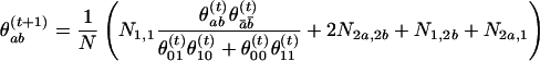in which ā = 1–a. These frequencies can be easily converted to a transition matrix. The algorithm usually converges very fast.

To test the effect of losing haplotype information among the controls, we simulated a control data set by randomly pairing up the given haplotypes in the CF control data set. To infer the location of the disease mutation (ΔF₅₀₈), we first used the EM algorithm to estimate the Markov transition matrices for the control group and then applied the BLADE algorithm. The posterior mean and 95% PI were 0.89 cM and [0.83, 0.94] cM, respectively, almost identical to the case when the control haplotypes were available (Liu et al. 2001).

Determining the Number of Clusters

Following Liu et al. (2001), we assume that the disease haplotypes can be grouped into k+1 clusters corresponding to k founder chromosomes in the current disease population and one null cluster for all other disease chromosomes. Each non-null cluster is characterized by an ancestral haplotype associated with a single disease-causing mutation coalescing to a single time point (age). Although the cluster number k has a significant effect on the estimation results, its determination is still an outstanding issue. A feasible strategy is to use the maximum a posterior (MAP) criterion. That is, we choose k so as to maximize the joint posterior distribution:

in which A is the set of ancestral haplotypes, G the vector of numbers of generations from the ancestral mutations, and θ the location of the disease mutation. The explicit forms of the likelihood function and prior distributions are given in Liu et al. (2001).

References

- Abecasis, G.R. and Cookson, W.O. 2000. GOLD—graphical overview of linkage disequilibrium. Bioinformatics 16: 182–183. [DOI] [PubMed] [Google Scholar]
- Akey, J.M., Zhang, K., Xiong, M., Doris, P., and Jin, L. 2001. The effect that genotyping errors have on the robustness of common linkage-disequilibrium measures. Am. J. Hum. Genet. 68: 1447–1456. [DOI] [PMC free article] [PubMed] [Google Scholar]
- Chiano, M.N. and Clayton, D.G. 1998. Fine genetic mapping using haplotype analysis and the missing data problem. Ann. Hum. Genet. 62: 55–60. [DOI] [PubMed] [Google Scholar]
- Clark, A.G. 1990. Inference of haplotypes from PCR-amplified samples of diploid populations. Mol. Biol. Evol. 7: 111–122. [DOI] [PubMed] [Google Scholar]
- Clark, V.J., Metheny, N., Dean, M., and Peterson, R.J. 2001. Statistical estimation and pedigree analysis of CCR2-CCR5 haplotypes. Hum. Genet. 108: 484–493. [DOI] [PubMed] [Google Scholar]
- Excoffier, L. and Slatkin, M. 1995. Maximum-likelihood estimation of molecular haplotype frequencies in a diploid population. Mol. Biol. Evol. 12: 921–927. [DOI] [PubMed] [Google Scholar]
- Fallin, D. and Schork, N.J. 2000. Accuracy of haplotype frequency estimation for biallelic loci, via the expectation-maximization algorithm for unphased diploid genotype data. Am. J. Hum. Genet. 67: 947–959. [DOI] [PMC free article] [PubMed] [Google Scholar]
- Fallin, D., Cohen, A., Essioux, L., Chumakov, I., Blumenfeld, M., Cohen, D., and Schork, N.J. 2001. Genetic analysis of case/control data using estimated haplotype frequencies: Application to APOE locus variation and Alzheimer's disease. Genome Res. 11: 143–151. [DOI] [PMC free article] [PubMed] [Google Scholar]
- Gabriel, S.B., Schaffner, S.F., and Nguyen, H. 2002. The structure of haplotype blocks in the human genome. Science 296: 2225–2229. [DOI] [PubMed] [Google Scholar]
- Gerdes, L.U., Gerdes, C., Hansen, P.S., Klausen, I.C., Færgeman, O., and Dyerberg, J. 1996, The apolipoprotein E polymorphism in Greenland Inuit in its global perspective. Hum Genet. 98: 546–550. [DOI] [PubMed] [Google Scholar]
- Hanlon, C.S. and Rubinsztein, D.C. 1995. Arginine residues at codons 112 and 158 in the apolipoprotein E gene correspond to the ancestral state in humans. Atherosclerosis 112: 85–90. [DOI] [PubMed] [Google Scholar]
- Hawley, M.E. and Kidd, K.K. 1995. HAPLO: A program using the EM algorithm to estimate the frequencies of multi-site haplotypes. J. Hered. 86: 409–411. [DOI] [PubMed] [Google Scholar]
- Hodge, S.E., Boehnke, M., and Spence, M.A. 1999. Loss of information due to ambiguous haplotyping of SNPs. Nat. Genet. 21: 360–361. [DOI] [PubMed] [Google Scholar]
- Hoh, J. and Hodge, S.E. 2000. A measure of phase ambiguity in pairs of SNPs in the presence of linkage disequilibrium. Hum. Hered. 50: 359–364. [DOI] [PubMed] [Google Scholar]
- International Human Genome Sequencing Consortium. 2001. Initial sequencing and analysis of the human genome. Nature 409: 860–921. [DOI] [PubMed] [Google Scholar]
- Jeffreys, A.J., Kauppi, L., and Neumann, R. 2001. Intensely punctate meiotic recombination in the class II region of the major histocompatibility complex. Nat. Genet. 29: 217–222. [DOI] [PubMed] [Google Scholar]
- Kerem, B., Rommens, J.M., Buchanan, J.A., Markiewicz, D., Cox, T.K., Chakravarti, A., Buchwald, M., and Tsui, L.C. 1989. Identification of the cystic fibrosis gene: Genetic analysis. Science 245: 1073–1080. [DOI] [PubMed] [Google Scholar]
- Liu, J.S., Sabatti, C., Teng, J., Keats, B.J.B., and Risch, N. 2001. Bayesian analysis of haplotypes for linkage disequilibrium mapping. Genome Res. 11: 1716–1724. [DOI] [PMC free article] [PubMed] [Google Scholar]
- Long, J.C., Williams, R.C., and Urbanek, M. 1995. An EM algorithm and testing strategy for multiple-locus haplotypes. Am. J. Hum. Genet. 56: 799–810. [PMC free article] [PubMed] [Google Scholar]
- Mahley, R.W. and Rall Jr., S.C. 2000. Apolipoprotein E: Far more than a lipid transport protein. Annu. Rev. Gen. Hum. Genet. 1: 507–537. [DOI] [PubMed] [Google Scholar]
- Martin, E.R., Lai, E.H., Gilbert, J.R., Rogala, A.R., Afshari, A.J., Riley, J., Finch, K.L., Stevens, J.F., Livak, K.J., Slotterbeck, B.D., et al. 2000. SNPing away at complex diseases: Analysis of single-nucleotide polymorphisms around APOE in Alzheimer disease. Am. J. Hum. Genet. 67: 383–394. [DOI] [PMC free article] [PubMed] [Google Scholar]
- McPeek, M.S. and Strahs, A. 1999, Assessment of linkage disequilibrium by the decay of haplotype sharing, with application to fine-scale genetic mapping. Am. J. Hum. Genet. 65: 858–875. [DOI] [PMC free article] [PubMed] [Google Scholar]
- Morris, A.P., Whittaker, J.C., and Balding, D.J. 2002. Fine-scale mapping of disease loci via shattered coalescent modeling of genealogies. Am. J. Hum. Genet. 70: 686–707. [DOI] [PMC free article] [PubMed] [Google Scholar]
- Niu, T., Qin, Z.S., Xu, X., and Liu, J.S. 2002. Bayesian haplotype inference for multiple linked single-nucleotide polymorphisms. Am. J. Hum. Genet. 70: 157–169. [DOI] [PMC free article] [PubMed] [Google Scholar]
- Qin, Z.S., Niu, T., and Liu, J.S. 2002. Partition-ligation EM algorithm for haplotype inference with single nucleotide polymorphisms. Am. J. Hum. Genet. 71: 1242–1247. [DOI] [PMC free article] [PubMed] [Google Scholar]
- Rocchi, A., Pellegrini, S., Siciliano, G., and Murri, L. 2003. Causative and susceptibility genes for Alzheimer's disease: A review. Brain Res Bull. 61: 1–24. [DOI] [PubMed] [Google Scholar]
- Stephens, M., Smith, N.J., and Donnelly, P. 2001. A new statistical method for haplotype reconstruction from population data. Am. J. Hum. Genet. 68: 978–989. [DOI] [PMC free article] [PubMed] [Google Scholar]
WEB SITE REFERENCE
- http://www.fas.harvard.edu/junliu/TechRept/03folder/bladev2.tgz; An improved version of the program BLADE v2.