COMPUTERIZED TRAINING OF CRYOSURGERY – A SYSTEM APPROACH

Abstract

The objective of the current study is to provide the foundation for a computerized training platform for cryosurgery. Consistent with clinical practice, the training process targets the correlation of the frozen region contour with the target region shape, using medical imaging and accepted criteria for clinical success. The current study focuses on system design considerations, including a bioheat transfer model, simulation techniques, optimal cryoprobe layout strategy, and a simulation core framework. Two fundamentally different approaches were considered for the development of a cryosurgery simulator, based on a finite-elements (FE) commercial code (ANSYS) and a proprietary finite-difference (FD) code. Results of this study demonstrate that the FE simulator is superior in terms of geometric modeling, while the FD simulator is superior in terms of runtime. Benchmarking results further indicate that the FD simulator is superior in terms of usage of memory resources, pre-processing, parallel processing, and post-processing. It is envisioned that future integration of a human-interface module and clinical data into the proposed computer framework will make computerized training of cryosurgery a practical reality.

INTRODUCTION

Cryosurgery is the destruction of undesired tissues by freezing, with practical applications since the beginning of the 20^th century [33]. The development of cryosurgery as an invasive procedure started in 1961, when Cooper and Lee invented the first cryoprobe (then cryostat) based on liquid nitrogen boiling [6]. Contrary to common belief, the Joule-Thomson-based cryoprobe was presented shortly thereafter, which is essentially the temperature change resulting from a sudden relief of pressurized gas [7,32]. Ever since, the technology of cryosurgical devices has shown tremendous improvements, following trends of miniaturization while improving cooling capabilities. Dramatic developments in medical imaging in the 1980s eventually led to a quantum leap in cryosurgical practice in the early 1990s, from a superficial treatment (often combined with surgical excision) to an imaged-guided, minimally invasive procedure on the prostate [13,28]. While minimally invasive cryosurgery has been experimented on virtually every tissue of the body, the prostate was the first organ to be treated with this application, for which a wide database is already available [9,14,34].

The new minimally invasive procedure has presented new practical challenges associated with selecting the most effective cooling technology (i.e., liquid nitrogen versus Joule-Thomson cooling), optimizing the cryoprobe for its diameter and active length, optimizing the cryoprocedure for the total number of cryoprobes and their layout, and identifying the most effective cooling protocol (also known as thermal history). While the literature is saturated with clinical reports on best cryosurgery practices [10], often sponsored by device manufacturers, an unbiased holistic approach to cryosurgery planning and practice remains an unmet need.

It is the view of the authors that cryosurgery technology far surpassed cryosurgery practice, and that modern cryosurgery devices could be used at far higher levels of efficiency, effectiveness, and sophistication. Concurrent developments in computer hardware and computation techniques are likely to facilitate the next quantum leap in cryosurgery applications. A current barrier appears to be associated with the level complexity of the procedure, as optimizing cryosurgery is essentially a multi-parameter optimization process, where clinical constraints are intimately linked with technology limitations. For example, even when the cooling technology is predetermined for a particular procedure and the number of cryoprobes and their operational parameters are chosen, the optimal cryoprobe layout alone is a complex optimization problem [2,3,11,12]. Here, suboptimal cryoprobe layout may leave areas in the target region untreated, lead to cryoinjury of healthy surrounding tissues, increase the duration of the surgical procedure, and increase the likelihood of post-cryosurgery complications; all of which affect the quality and cost of the medical treatment. These shortcomings may further affect the quality and duration of clinical training, which is related to the subject matter of the current study.

A holistic approach to improve modern cryosurgery necessitates the development of computerized tools. For example, the current research team has devoted efforts in recent years to develop a computerized planning scheme for cryosurgery, based on bioheat transfer simulations. This scheme integrates a close-to-real-time bioheat simulation [22,23] with two planning algorithms, known as bubble packing [24,29] and force-field analogy [12,29]. The planning scheme has used an early prototype method for organ model reconstruction [30]. However, those prior efforts have aimed at developing the fundamental building blocks for computerized planning, while bypassing challenges associated with human-machine interface—the interface necessary for the clinician to effectively use the computer code. Challenges in human-machine interaction for a minimally invasive thermal procedure arise from the need to combine medical imaging data with thermal data, while simulating the clinical procedure.

As a part of our ongoing program to develop a computerized training tool for cryosurgery, the objective of the current study is to provide the foundation for a computerized training platform for cryosurgery, while benchmarking and integrating previously developed building blocks [12,22-24,29,30]. Developing the human-interface module [27] and integration of clinical data on the abnormal growth of the organ with the progress of the disease [26] are subject matters of parallel efforts. The current study demonstrates that a finite-difference based bioheat simulation core, integrated into a parallel-processing computation framework, can meet the need of computerized planning and training in a clinically relevant time scale. It is envisioned that future integration of those key elements will enable computerized training of cryosurgery in a virtual setup.

SYSTEM DESIGN – COMPUTERIZED TRAINER

With reference to Fig. 1, the Trainer proposed in the current study is composed of a graphical user interface (GUI), which accesses three modules: Tutor, Simulator, and Database. The Tutor module presents the user with sample surgery cases and relevant information, allows the user to select a suggested cryoprobe layout, displays a computer-generated optimal layout, and provides feedback on how the user could improve performance. The Tutor module uses the Simulator to simulate a procedure based on relevant data selected from the Database. The Simulator simulates both the bioheat transfer process during cryosurgery and also the clinical operation via imaging guidance. The Simulator returns the thermal history in the target region to the Tutor, in order to evaluate the effectiveness of the specific surgical case. Following an optimization scheme, the Tutor may execute the Simulator multiple times with variable input datasets, until a preferred simulated protocol is identified. At the end of each simulation, the thermal history is stored in the Database, together with the evaluation of results by the Tutor.

Figure 1.

Structural design of the cryosurgery training code

Examples of the data structures stored in the Database in conjunction with a particular case are: ultrasound voxel data of the organ to be treated, volumetric prostate models, thermal history of simulated procedure, history of cryoprobe insertion, cryoprobe operational parameters, and the planning objectives for the particular case study. At the end of each tutoring session, the new data generated during the session is added to the Database. Database management, exchange with the Tutor and Simulator, presentation, and interaction with the trainee is the subject of a parallel study [27]. Developing credible 3D prostate models and combining clinical data on the progression of the disease in the organ is the subject matter of a different parallel study [26]. The current study focuses on developing, benchmarking, and optimizing an efficient bioheat simulation core, to serve as the mainstay of the simulator. This effort is done in concert with parallel studies, to ensure compatibility and efficiency in data sharing, all internally-controlled by the various modules of the computerized tool.

In order to make the Simulator educationally relevant, it should be able to perform a complete thermal simulation of a cryosurgery procedure in a relatively short period, in the order of a few minutes. Given the computation-intensive nature of simulating bioheat transfer with phase change, and available computer platforms, the bioheat transfer simulation core of the Simulator must be designed for parallel computing on a multi-core machine.

Three key system elements are described below, with implications to system design: the bioheat transfer model, the simulation technique, and the optimal cryoprobe layout strategy. In the subsequent section, results and discussion are presented for the integrated system.

Bioheat Transfer Model

For the purpose of platform development, heat transfer during cryosurgery is modeled after the classical bioheat equation [15]:

$$C\frac{\partial T}{\partial t}=\nabla (k\nabla T)+{\stackrel{.}{w}}_b{C}_b(T_b-T)+{\stackrel{.}{q}}_{\mathit{met}}$$ (1)

where C is the volumetric specific heat, T is the tissue temperature, t is the time, k is thermal conductivity of the tissue, ${\stackrel{.}{w}}_b$ is the blood perfusion volumetric flow rate per unit volume of tissue, C_b is the volumetric specific heat of blood, T_b is the blood temperature entering the thermally treated area, and ${\stackrel{.}{q}}_{\mathit{met}}$ is the metabolic heat generation.

Numerous scientific reports have been published studying the mathematical consistency and validity of the above classic equation, while exploring various alternatives (for example, see Charny [5] and Diller [8]). It is assumed in the current study that a more advanced model of bioheat transfer will not warrant higher accuracy in the cryosurgery simulation, will involve greater mathematical complications, and is deemed unnecessary in the current study. Note that metabolic heat generation is typically negligible compared to the heating effect of blood perfusion, and is neglected in this study [16]. Discussion with regard to the applicability of this equation to prostate cryosurgery simulations is presented in [16,22-24]. Nevertheless, the computerized platform proposed in the current study is insensitive to the actual heat transfer model applied.

While selecting the most appropriate governing equation may be a valid point for debate, one must bear in mind that the numerical framework described in the current study is aimed at stimulating a minimally invasive clinical procedure. As such, it is emphasized that (i) reconstruction of the topology of blood vessels from medical imaging in a clinical setup is impractical, (ii) parametric estimation of blood flow in each blood vessel, in real time, is impractical even when the topology is known, and (iii) the overall contribution of the above level of detail to the evaluation of the freezing front location is in the order of 10% [16]. Hence, Eq. (1) is deemed an adequate choice of practice.

Typical thermal properties used for cryosurgery simulation in the current study are listed in Table 1. Since the effect of metabolic heat generation is at least one order of magnitude smaller than the heating effect due to blood perfusion, this term is neglected [17] in the current study. It is further noted that the heating effect of blood perfusion may affect the size of the frozen region by about 5% in a typical time frame of a cryosurgical procedure [16]. Assuming that the tissue can be first-order approximation as a NaCl solution in the current study, phase-transition temperature range is assumed between 0°C and −22°C.

Table 1.

Representative thermophysical properties of biological tissues used in the current study [9].

Thermophysical Property	Value (T in degree K)
Thermal conductivity, k, W/m·K	0.5 15.98-.0567×T 1005×T−1.15	273<T 251<T<273 T<251
Volumetric specific heat, C, MJ/m3·K	3.6 880-3.21×T 2.017×T-505.3 0.00415×T	273<T 265<T<273 251<T<265 T<251
Latent heat, L, MJ/ m3	300
Blood perfusion heating effect, wbCb, kW/ m3·K	40 0	273<T T<273

Consistent with the thermal analysis presented by Rossi et al. [23], prostate cryosurgery is simulated in an infinite domain from heat transfer considerations, subject to an initial temperature of 37°C. As discussed there, a finite domain having dimensions of about three times greater than that of the prostate can be considered infinite for cryosurgery simulations. Internal boundary conditions at the cryoprobe surface are: a constant cooling rate from 37° C to −145°C within 30 seconds, followed by a constant temperature of −145°C.

Bioheat Simulation Techniques

Conceptually, at least two approaches could be applied for bioheat simulations, using either finite-elements (FE) analysis or finite-difference (FD) scheme, where discussions about the preferred approach attract significant attention in professional meetings [19-21,28]. When an FE approach is taken, one could use a commercial code which may guaranty robustness and user friendliness. Equally important are efficiency in calculations and short runtime, where an FD scheme may be of superior performance. While the application of a particular numerical scheme may simply be a matter of personal preference, the application of commercial software versus a proprietary code may carry further implications on the cost and complexity of development. From considerations of cost, efficiency, availability, development time, user friendliness, and robustness, it appears to the authors that a commercial code would be a better choice for the current development, should the FE approach is to be taken. By contrast, developing a proprietary code would be required should the FD approach be taken. Of course, the opinion of other developers in the field may vary based on their own experience and record of achievements, and they may wish to explore additional methods, should they be challenged with the task of developing competitive computerized platforms. It was therefore warranted that both simulation approaches be investigated in the current study.

For the purpose of development in the current study, two bioheat transfer simulation cores were benchmarked, using the FE commercial code ANSYS [1] and a proprietary FD code presented previously [23]. Table 2 lists key comparison points for those alternatives, where more discussion on the pros and cons of these applications is provided in the Discussion section. While some of the comparison criteria are unique to the current selection, many others are quite general. It is acknowledged that other FE commercial codes could be used, but comparison of the various commercial codes is beyond the scope of the current study. Nevertheless, based on the authors’ experience and the literature, ANSYS would serve the objectives of this comparison adequately. It is further acknowledged that other FD schemes could also be used for heat transfer simulations [4]. Nevertheless, the scheme presented by Rossi et al. [23] has already been demonstrated superior for the purpose of cryosurgery simulations. This FD scheme has been further verified against experimental data on gelatin solution [22,35], based on 24 independent experiments in eight representative cryoprobe layouts (n=3). Results of that study indicated an average uncertainty of 0.4 mm in freezing front location, and a mismatch of less than 5% between the simulated and the measured frozen region areas (average mismatch value of 2.9% from all experiments). By comparison, identifying the freezing front location by means of medical imaging is estimated to be not better than 1 mm. More information about the expected level of certainty during a clinical procedure is included in Results and Discussion.

Table 2.

Comparison of a FE simulator based on ANSYS [26] and a proprietary FD simulator [17].

Comparison Criteria	FE-Based Simulator		FD-Based Simulator
	Pros	Cons	Pros	Cons
Geometrical representation of complex shapes	Natural conformity of grid points to curved surfaces			Difficult with the more intuitive orthogonal grid system
Simulation of the classical bioheat equation		Requires a special operations to account for the heating effect due to blood perfusion	Similar difficulty to the ordinary conduction problem; blood perfusion increases system stability [15]
Computation cost at each time step		High, requires matrix solvers and high number of operations	Low for an explicit scheme, straightforward calculations
Memory resources		High demand, matrices size is orders of magnitude larger than the number of grid points	Low demand, matrices size and number of grid points are of the same order
Defect region calculations		Very high cost	Low, can be calculated simultaneously
Time step interval for bioheat simulation	Relatively long	Stability does not guaranty convergence nor consistency; have to be evaluated iteratively	Stability is a necessary and sufficient condition for convergence and consistency	Explicit formulation requires very small time steps to ensure stability
Computational Complexity	Linear with numerical grid points		Linear with numerical grid points
Pre-processing & Post-processing		Complex due to grid points registration	Trivial with an orthogonal grid system
Scalability	Parallel kernels possible	Bottlenecks due to matrices operation	Trivial for an explicit scheme, no bottlenecks
Availability of commercial codes for heat transfer simulations	A selection is available			None
User friendliness	High when an FE commercial code is used by a proficient user with technical background	Low when a commercial code is used by a novice user with no technical background	High when a proprietary code is tailored for a novice user from a medical background	Impractical without developing a tailored system

With the above acknowledgements in mind, it appears that the selection between the FE and the FD approaches to develop the bioheat transfer simulation core is not a trivial decision. This decision calls for benchmarking the two schemes as discussed below.

Optimal Cryoprobe Layout Strategy

Key to successful cryosurgery is appropriate selection of cryoprobe location, in order to maximize destruction to the target region while minimizing injury to surrounding tissues. As overviewed in the introduction, efforts have been devoted over the years to optimize the cryoprobe layout. Regardless of the optimization approach taken, a measure of the quality of planning must be defined. For the purpose of the current study, the concept of defect region, G, is adopted [12]:

$$G=\frac{1}{V_t}{\int }_{V_s}\mathit{wd}{V}_s;w=\{\begin{array}{c}\phantom{\{}\begin{array}{cc}\hfill 1\hfill & \hfill T_p<T\hfill \\ \hfill 0\hfill & \hfill T\le T_p\hfill \end{array}\}\text{interior to the target region}\hfill \\ \phantom{\{}\begin{array}{cc}\hfill 1\hfill & \hfill T\le T_p\hfill \\ \hfill 0\hfill & \hfill T_p<T\hfill \end{array}\}\text{exterior to the target region}\hfill \end{array}\phantom{\}}$$ (2)

where V_t is the volume of the target region, V_s is the volume of the simulated domain, w is a weight function, and T_p is the planning isotherm. For simplicity in presentation, a binary value is selected for the weight function in Eq. (2). The defect value varies throughout the simulated procedure: it starts with a value of one at the beginning of the procedure, when the entire target region is unfrozen, decreases as the freezing process progresses, gets to a minimum value when the internal defect becomes equal to the external defect (Fig. 2), and increases again as the external defect grows—up to limits dictated by the cooling power of the cryoprobes. The defect region concept is consistent with clinical practice, where the surgeon attempts to correlate the frozen region contour with the target region shape, using medical imaging. Monitoring the evolution of the defect region has major implications on the computation cost (Table 2).

Figure 2.

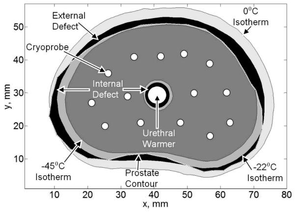
Temperature regions of interest for the purpose benchmarking in the current study.

The value of the planning isotherm, T_p, is probably one of the most debated planning parameters among cryosurgeons. Note that biological tissues change phase over a wide temperature range—0°C to −22°C. Furthermore, cryoinjury continues to progress below the boundaries of phase change down to the so-called lethal temperature, most frequently argued to be in the range of −40°C to −50°C. When T_p is selected to equal 0°C, the frozen region as would appear in medical imaging is optimized to match the contour of the target region. When T_p equals the lethal temperature value, the entire target region is optimized for maximum cryoinjury, while creating a significant injury to surrounding tissues. A compromise may be established by simply selecting T_p= −22°C, but T_p must be left as a free parameter for the purpose of training.

While identifying the optimal cryoprobe layout is a multi-parameter optimization problem, one or a combination of two alternatives may be employed: force-field analogy [12,18,29] and bubble-packing method [24,29-31]. In force-field analogy, the defect applies virtual forces on the cryoprobes at the end of each heat transfer simulation, displacing them to new locations that could potentially lower the defect in a consecutive simulation. Using the bubble-packing method, each cryoprobe is simulated by an ellipsoidal bubble, representing the affected region by a cryoprobe. Virtual van der Waals forces move the bubbles within the target region until they reach a layout of force equilibrium; the same layout is then adopted to place cryoprobes. By optimizing bubble parameters for the specific cryoprobes, a minimum defect layout can be identified. The typical runtime of the bubble-packing method is measured in seconds. If one wants to improve upon the layout established with bubble-packing, a force-field analogy phase may be followed, which is more computationally expensive—measured in the same scale as of the bioheat transfer simulation [29]. Most frequently, bubble-packing alone has shown to be an adequate planning method with no need for further optimization.

Simulator Framework

The simulator framework must be modular in nature, to enable data transfer with the other components of the training software package (Fig. 1), and to integrate alternative heat transfer simulation cores. As a requirement, the simulator must be able to evaluate defect values through the process of simulation. A schematic illustration of the heat transfer simulation framework is presented in Fig. 3. The description below highlights the FE implementation with ANSYS, where source code of the simulation core is unavailable. With reference to Fig. 3, the simulating core is naturally subdivided into: pre-processing, computing, post-processing, and a main control loop. In the pre-processing phase, three input files are read into the simulator: (i) “.sim” which contains the simulation settings, such as material properties, operational parameters, and cryoprobe layout; (ii) “.csv” which contains the numerical grid; and (iii) “.agf” which contains the 3D surface data of the target region—the prostate and urethra in the current study.

Figure 3.

Implementation of the FE bioheat transfer simulation core with ANSYS. Data transfer scheme is made identical for the FD simulator for the purpose of benchmarking.

The simulator core encapsulates two time cycles, the first is the sequence of time steps for progression of the numerical simulation, and the second is the periodic evaluation of the defect value. While the cost of defect evaluation is negligible for an FD scheme, and can be done in parallel, a FE scheme necessitates a post-processing phase for defect evaluation, which may create a bottleneck in calculations. Using ANSYS, the second cycle is performed by analyzing the results file “.rst” at the end of the cycle, following the execution of the commands listed in “.lgw”. In either simulator, heat transfer simulation progresses until a minimum defect is identified. Once the simulation terminates a “.srt” results file is generated, containing the temperature and defect history of the simulation domain, to be used by the Trainer and stored in the Database (Fig. 1). While the above process of file sharing and data transfer may appear cumbersome and computationally expensive, it is necessary in the development of the postprocessor functionality when integrating a commercial code structure.

RESULTS AND DISCUSSION

Benchmarking studies were performed on a cancerous prostate model created previously (Fig 4), using 14 cryoprobes at a uniform insertion depth, with optimal layout generated by bubble packing [30]. All simulations were performed on an Intel® i7-950 (four-core) machine, running at 3.07GHz, with 9GB of RAM. All heat transfer simulations were run for 255 seconds of simulated runtime, which coincides with the point of minimum defect for the FD-based code.

Figure 4.

Illustration of a fourteen-cryoprobe layout in the cancerous prostate model used in the current study for benchmarking. The urethral warmer—a cylindrical heater in the form of a catheter—is designed to protect the urethra from cryoinjury and is modeled as a heated tube.

It can be seen from Table 3 that the FD and FE schemes identify different values for the time to minimum defect, which is directly related to the way that the phase-transition temperature range is handled. Note that for both selected schemes, the freezing front location is interpolated from temperature data and it is not a parameter of the solution. It is also noted that the optimal cryoprobe layout has shown to be insensitive to the simulated time to minimum defect—computationally [23] and experimentally [24]. Based on the high certainty in predicting the freezing from location with the FD solution (0.4 mm, see Bioheat Simulation Technique, above), and given the fact that stability is a necessary and sufficient condition for convergence in the particular FD scheme [4], we conclude that the FE results in Table 3 come with lower certainty than the benchmark solution.

Table 3.

Benchmarking results of the FE and FD simulators on a representative case of a cancerous prostate model. Cryoprobe layout is based on a bubble packing method (illustrate d in Fig. 4). For the FE simulator, a time step of the 60 sec represents an upper limit for convergence, whereas the 30 sec time step is deemed practical for concurrent defect region calculations. Time step for the FD simulator is taken at the stability li mit.

Simulator	FE		FD
Time step		60 sec	30 sec	.02 sec
Minimum defect value		24.5%	24.7%	24.3%
Total simulated time		255 sec	255 sec	255 sec
Simulated time to minimum defect		180 sec	199 sec	255 sec
Actual runtime	1 core	613 sec	966 sec	144 sec
	2 cores	423 sec	689 sec	83 sec
	4 cores	304 sec	521 sec	67 sec
Simulated time ratio = comp. runtime / procedure duration	1 core	236%	379%	56%
	2 cores	165%	270%	32%
	4 cores	119%	204%	26%

Figure 5 displays the resulting temperature field at the point of minimum defect, where Fig. 6 displays the evolution of the defect for the same simulation. Comparison of advantages and disadvantages in using the FE and FD simulators is listed in Table 2, based on the specifics of benchmarking. Furthermore, Table 3 lists simulation results for parallel computation on a number of cores ranging from one to four, for the same cryosurgery case displayed in Fig. 5.

Figure 5.

Temperature field at the point of minimum defect: (left) temperature field superimposed on the prostate outer surface; (right) cross section passing through the center of the active surface of the cryoprobes.

Figure 6.

Evolution of total defect for the simulated case displayed in Fig. 5

Before benchmarking can take place, the FE simulation core must be optimized for runtime while maintaining acceptable accuracy. Due to the large number of parameters, a sequential optimization process was performed for: (1) mesh size, (2) time step size, and (3) solver type and associated convergence tolerance. An acceptable accuracy level in all optimization steps was considered to be 2 mm in the location of the freezing front, which corresponds to about 3% change in frozen region volume in most cases. Such an error in freezing front location coincides with the uncertainty range with medical imaging—the sum of imaging resolution of 1 mm and 1 mm positional error in the process of shape reconstruction. The accuracy in freezing front location was evaluated by a comparison with a base case, which was selected as a converged solution that matched the results of the FD simulation core (discussed in [23] and compared with experimental results in [22]). In addition, the average temperature difference within the frozen region was also investigated to ensure the convergence of the temperature-field. The optimization test cases were based on fourteen cryoprobes in a layout optimized with bubble packing, for a realistic cancerous prostate geometry. The test case was run until minimum defect had occurred for each parameter choice for identical cryoprobe layouts.

FE optimization for mesh size

In order to select the optimal mesh distribution, mesh sizes are set on various control surfaces within the model, then the mesh size is interpolated within the volume between the surfaces. Selected mesh surfaces include the active cooling portion of the cryoprobes (1 mm), the heated area of the urethral warmer (3 mm), the prostate contour (5 mm), and the external boundary of the simulated domain (10 mm); those numerical values are scaled with the respective temperature gradients. The mesh convergence study was carried out by proportionally increasing the mesh on all of the above surfaces, until the limits of accuracy criteria were identified, where a tetrahedral mesh was found to best populate the domain defined by those surfaces.

FE optimization for time step

One minute is deemed the largest allowable interval between simulation results for effective planning from defect-calculation considerations. As specified above, the thermal history of the cryoprobes consists of a rapid cooling stage and cryogenic temperature hold stage. Consistently, the freezing front grows at a faster rate at the beginning of the procedure. The two-stage cooling protocol was matched with a simulation scheme based on two time step intervals. Figure 7 displays selected results of the time step convergence study, where the average temperature difference within the frozen region (temperatures below 0°C) is calculated with reference to the FD solution. It can be seen from Fig. 7 that the average temperature difference is initially large, due to the small volume of the frozen region and the high temperature gradients surrounding the cryoprobes; that temperature difference monotonically decays as the simulated process approaches steady state. Since the early stage of freezing plays a lesser role in evaluating the effects of the cryoprocedure, time step intervals of 10 sec during cryoprobe cooling and 60 sec during cryogenic temperature hold period are found acceptable for the purpose of the current study. While the 60 sec interval is deemed adequate for the numerical solution, the parallel search for minimum defect necessitated intermediate values, which eventually led the investigation to also include 30 sec intervals. This illustrates a difficulty in integrating a commercial code for heat transfer simulations with parallel calculations for the quality of simulation.

Figure 7.

Average temperature difference in the frozen region (T<0°C) between the FE and FD simulation results, for an FD time step of 0.02 sec and various FE time intervals: Δt_c is the time step during cryoprobe cooling from 37°C to −145°C, and Δt_h is the time step size when the cryoprobe temperature is held at −145°C.

FE optimization for numerical solver and convergence tolerance

For the above mesh selection and time intervals, the following solvers were tested: Sparse Solver, an Advanced Multigrid Solver, a proprietary preconditioned solver (conjugate gradient), a Jacobi Solver (conjugate gradient), and an Incomplete Cholesky Conjugate Gradient Solver (ICCGS). Most effective was found the ICCGS, running at least 8% faster than any other tested solver (infinity norm=10⁻⁶ for Newton-Raphson tolerance).

Computational Complexity

As could be expected from theoretical analysis of the FE scheme, Fig. 8 displays almost linear increase in complexity with the increased number of nodes and, independently, with the increased number of cryoprobes (i.e., increased surface area of fine mesh). The deviation from linearity is resulted from changes in the cryoprobe layout when the number of cryoprobes varies in the same selected domain. A linear computational complexity for the FD scheme has been demonstrated previously with the increasing cryoprobes number [23].

Figure 8.

Computation time of the FE simulator as a function of the number of cryoprobes N_P, and for the corresponding number of nodes N_N using optimal mesh sizes, for cryoprobe layouts determined using bubble packing.

Scalability

For the case of 30 sec FE time step, the FD simulator is about 6.7 to 8.3 times faster than the FE simulator (Table 3). Given the fact that the FD simulator actually advances in time steps in the order of 10⁻² sec, this result is extraordinary. The reason for the superiority of the FD runtime is in its explicit formulation, where the short time interval is traded with simplicity in calculation. With regard to defect calculations, the 30 sec intervals of the FE simulator may lead to unnecessary simulation time, whereas the small time intervals of the FD simulator provides continues information of the defect region progression.

Multi-Core Processing

While one could expect the simulation runtime to be inversely proportional to the number of computation cores in parallel processing, increasing the number of computation cores from 1 to 4 reduces simulation runtime by a factor of 2 for both the FD and FE schemes (Table 3), but from different reasons (both codes are specifically written for parallel processing). For the FD simulator, suboptimal acceleration is primarily due to the i7 chip architecture, where all the cores share the same amount of L3 cache in parallel computing as one core would use in a single core run. For the FE simulator, the suboptimal acceleration is primarily due to the sequential steps necessary for the complex pre- and post-processing. Due to the explicit nature of the FD scheme, it is an excellent candidate for parallel computing, providing that the amount of L3 cache is large enough. It is concluded that with increased cache size, the FD scheme runtime will become inversely scale with the number of cores, which represents a significant advantage with the current trend of increased number of computation cores on personal computers (six and eight cores are already widely available on mid-range machines).

Geometry representation

An area in which the FE simulator is superior to the FD simulator is that of geometrical modeling fidelity. The FD simulator is restricted to placing nodes on a rectilinear grid, which necessitates a finer discretization to represent the non-rectangular geometry of the prostate. By contrast, the FE method has fewer restrictions on node placement and, thereby, the pre-processor of the commercial code is able to represent a complex shape with fewer nodes. For the current test case, approximately 95,000 nodes were needed for the FD simulator as opposed to 80,000 nodes for the FE simulator to obtain an accurate solution. Despite the apparent superior geometrical representation in the FE simulations, the FD simulator displayed a higher accuracy in temperature field calculations, which was obtained in a shorter runtime.

Key development objectives for the cryosurgery trainer are short runtime on a personal computer and user friendliness in operation, in order to make the trainer application practical for a large community of novice users. Given the computation cost of the bioheat transfer simulation with phase change, meeting this objective requires innovation in code writing and selection of an efficient computer framework. Given the computation cost and recent developments in computer hardware, it appears that we are currently at the verge of meeting those development objectives with the FD simulation core.

SUMMARY AND CONCLUSIONS

As a part of our ongoing program to develop a computerized training tool for cryosurgery, the objective of the current study is to provide the foundation for a computerized training platform for cryosurgery. Key elements of the developing training platform are a simulator, a tutor, and a database. The current study focuses on system design considerations, including the bioheat transfer model, bioheat simulation techniques, optimal cryoprobe layout strategy, and the simulation core framework.

Two fundamentally different approaches were considered for the development of a cryosurgery simulator in the current study, by integration with either an FE commercial code (ANSYS) or a proprietary FD code. While a wide selection of FE commercial codes could be selected and, independently, a wide range of FD schemes could be adopted, the significance of the current study is in the comparison of the two fundamentally different approaches. Nonetheless, to the opinion of the authors, each alternative is an excellent (and maybe the best) candidate for the task in its own category.

Benchmarking studies were performed on a cancerous prostate model created previously, using 14 cryoprobes at a uniform insertion depth, with optimal layout suggested by a bubble-packing optimization method. Benchmarking data were developed on a mid-range, four-core machine, which is commonly available in hospitals and medical clinics. Results of this study indicate that the FE simulator is superior in terms of geometric modeling, while the FD simulator is superior in terms of runtime. Benchmarking results also indicate that the FD simulator is superior in terms of memory resources, defect region calculations, pre-processing, post-processing, and multi-core processing. While both the FE and FD simulators operated on an identical computation framework, the fact that the FD simulator is a tailor-made code further puts it in a superior position in terms of user friendliness and efficiency in operation.

Parallel efforts of developing a human-interface module, and integration of clinical data on the abnormal growth of the organ with the progress of the disease, are currently underway and are the subject matters of parallel efforts. It is envisioned that future integration of those key elements into the proposed computer framework will make computerized training of cryosurgery a practical reality.

REFERENCES

- 1.ANSYS Inc. http://www.ansys.com/
- 2.Baissalov R, Sandison GA, Donnelly BJ, Saliken JC, McKinnon JG, Muldrew K, Rewcastle JC. Physics in Medicine and Biology. 2000;45:1085–98. doi: 10.1088/0031-9155/45/5/301. [DOI] [PubMed] [Google Scholar]
- 3.Baissalov R, Sandison GA, Reynolds D, Muldrew K. Physics in Medicine and Biology. 2001;46:1799–1814. doi: 10.1088/0031-9155/46/7/305. [DOI] [PubMed] [Google Scholar]
- 4.Carnahan B, Wilkes JO, Luther HA. Applied Numerical Methods. John Wiley & Sons; 1969. [Google Scholar]
- 5.Charny KC. In: Advances in Heat Transfer. Hartnett JP, Irvine TF, Cho YI, editors. Academic Press; 1992. pp. 19–156. [Google Scholar]
- 6.Cooper I, Lee A. Journal of Nerve and Mental Disease. 1961;133:259–266. [PubMed] [Google Scholar]
- 7.Crump RE, Reynolds FL, Tillstorm CR. 3,613,689 US Patent. 1971
- 8.Diller KR. In: Advances in Heat Transfer. Hartnett JP, Irvine TF, Cho YI, editors. Academic Press; 1992. pp. 1157–358. [Google Scholar]
- 9.Han KR, Cohen JK, Miller RJ, Pantuck AJ, Freitas DG, Cuevas CA, Kim HL, Lugg J, Childs SJ, Shuman B, Jayson MA, Shore ND, Moore Y, Zisman A, Lee JY, Ugarte R, Mynderse LA, Wilson TM, Sweat SD, Zincke H, Belldegrun AS. Journal of Urology. 2003;170:1126–1130. doi: 10.1097/01.ju.0000087860.52991.a8. [DOI] [PubMed] [Google Scholar]
- 10.Gage AA, Baust J. Cryobiology. 1998;37(3):171–186. doi: 10.1006/cryo.1998.2115. [DOI] [PubMed] [Google Scholar]
- 11.Keanini RG, Rubinsky B. ASME Journal of Heat Transfer. 1992;114:796–802. [Google Scholar]
- 12.Lung DC, Stahovich TF, Rabin Y. Computer Methods in Biomechanics and Biomedical Engineering. 2004;7:101–110. doi: 10.1080/10255840410001689376. [DOI] [PubMed] [Google Scholar]
- 13.Onik GM, Cohen JK, Reyes GD, Rubinsky B, Chang Z, Baust J. Cancer. 1993;72:1291–1299. doi: 10.1002/1097-0142(19930815)72:4<1291::aid-cncr2820720423>3.0.co;2-i. [DOI] [PubMed] [Google Scholar]
- 14.Onik GM. Cancer Control. 2001;8:522–531. doi: 10.1177/107327480100800607. [DOI] [PubMed] [Google Scholar]
- 15.Pennes HH. Journal of Applied Physiology. 1948;1:93–122. doi: 10.1152/jappl.1948.1.2.93. [DOI] [PubMed] [Google Scholar]
- 16.Rabin Y, Shitzer A. ASME Journal of Biomechanical Engineering. 1998;120:32–37. doi: 10.1115/1.2834304. [DOI] [PubMed] [Google Scholar]
- 17.Rabin Y. Cryobiology. 2003;46(2):109–120. doi: 10.1016/s0011-2240(03)00015-4. [DOI] [PubMed] [Google Scholar]
- 18.Rabin Y, Lung DC, Stahovich TF. Technology in Cancer Research and Treatment. 2004;3:227–243. doi: 10.1177/153303460400300301. [DOI] [PubMed] [Google Scholar]
- 19.Rabin Y, Tanaka D, Shimada K. Proceedings of Cryosurgery in the Americas; Montreal, Canada. September 25-26.2004. [Google Scholar]
- 20.Rabin Y. Clinical and Basic Science of Cryotherapy. Society for Thermal Medicine Annual Meeting; Washington, DC. May 14-17.2007. [Google Scholar]
- 21.Rabin Y. Computation tools in the service of cryosurgery. Society for Thermal Medicine Annual Meeting; Portland, OR. April 13-16.2012. [Google Scholar]
- 22.Rossi MR, Rabin Y. Physics in Medicine and Biology. 2007;52:4553–4567. doi: 10.1088/0031-9155/52/15/013. [DOI] [PMC free article] [PubMed] [Google Scholar]
- 23.Rossi MR, Tanaka D, Shimada K, Rabin Y. Computer Methods and Programs in Biomedicine. 2007;85:41–50. doi: 10.1016/j.cmpb.2006.09.014. [DOI] [PMC free article] [PubMed] [Google Scholar]
- 24.Rossi MR, Tanaka D, Shimada K, Rabin Y. International Journal of Heat and Mass Transfer. 2008;51:5671–5678. doi: 10.1016/j.ijheatmasstransfer.2008.04.045. [DOI] [PMC free article] [PubMed] [Google Scholar]
- 25.Rubinsky B, Gilbert JC, Onik GM, Roos MS, Wong STS, Brennan KM. Cryobiology. 1993;30(2):191–199. doi: 10.1006/cryo.1993.1019. [DOI] [PubMed] [Google Scholar]
- 26.Sehrawat A, Shimada K, Rabin Y. ASME 2011 Summer Bioengineering Conference; Farmington, PA, USA, 53205. 2011. [Google Scholar]
- 27.Shimada K, Furuhata T, Song I, Sehrawat A, Rabin Y. Cryobiology. 2011;63(3):315–316. [Google Scholar]
- 28.Thaokar C, Rabin Y. ASME 2011 Summer Bioengineering Conference - SBC 2011; Farmington, PA, USA. June 22-25.2011. [Google Scholar]
- 29.Tanaka D, Shimada K, Rabin Y. ASME Journal of Biomechanical Engineering. 2006;128:49–58. doi: 10.1115/1.2136166. [DOI] [PMC free article] [PubMed] [Google Scholar]
- 30.Tanaka D, Ross MR, Shimada K, Rabin Y. International Journal of Medical Robotics and Computer Assisted Surgery. 2007;3:10–19. doi: 10.1002/rcs.124. [DOI] [PMC free article] [PubMed] [Google Scholar]
- 31.Tanaka D, Shimada K, Rossi MR, Rabin Y. Computer Aided Surgery. 2008;13:1–13. doi: 10.3109/10929080701882556. [DOI] [PubMed] [Google Scholar]
- 32.Torre D. Journal of Dermatologic Surgery. 1975;1:56–58. doi: 10.1111/j.1524-4725.1975.tb00073.x. [DOI] [PubMed] [Google Scholar]
- 33.Whitehouse HH. Journal of the American Medical Association. 1907;49:371–377. [Google Scholar]
- 34.Wong WS, Chinn DO, Chinn M, Chinn J, Tom WL. Cancer. 1997;79:963–974. [PubMed] [Google Scholar]
- 35. http://www.andrew.cmu.edu/user/yr25/ExperimentalVerification.htm.