JIM-13-0560 R1: Propensity scores for confounder adjustment when assessing the effects of medical interventions using non-experimental study designs

Abstract

Treatment effects, especially when comparing two or more therapeutic alternatives as in comparative effectiveness research, are likely to be heterogeneous across age, gender, co-morbidities, and co-medications. Propensity scores (PSs), an alternative to multivariable outcome models to control for measured confounding, have specific advantages in the presence of heterogeneous treatment effects. Implementing PSs using matching or weighting allows us to estimate different overall treatment effects in differently defined populations. Heterogeneous treatment effects can also be due to unmeasured confounding concentrated in those treated contrary to prediction. Sensitivity analyses based on PSs can help to assess such unmeasured confounding. PSs should be considered a primary or secondary analytic strategy in non-experimental medical research, including pharmacoepidemiology and non-experimental comparative effectiveness research.

Randomized controlled trials (RCTs) are considered the gold standard for assessing the efficacy of medical interventions, including medications, medical procedures, and clinical strategies. Nevertheless, particularly for research on the prevention of chronic disease, RCTs are often not feasible because of the size that would be required to address rare outcomes, timeliness, budget requirements, and ethical constraints [1]. Non-experimental studies of medical interventions are not subject to these limitations, but have frequently been criticized because of their potential for confounding bias [2, 3]. This concern reached a crescendo with the disparity in estimated effects of postmenopausal hormone therapy on the risk for cardiovascular events from RCTs and non-experimental studies.[4] These discrepancies highlighted the need to develop and apply improved methods to reduce bias in non-experimental studies in which confounding is likely [5].

Rosenbaum and Rubin [6] developed the method of the propensity score (PS) as an alternative to multivariable outcome models for confounding control in cohort studies. PSs have become increasingly popular to control for measured confounding in non-experimental (epidemiologic or observational) studies that assess the outcomes of drugs and medical interventions [7]. While not generally superior to conventional outcome models [8], PSs focus on the design of non-experimental studies rather than the analysis [9]. Combined with the new user design [10], PSs specifically focus on decisions related to initiation of treatment and hypothetical interventions [11].

By comparing the distribution of PSs between the treated and untreated cohorts, PSs permit ready assessment to determine whether or not the treated and untreated patients are fully comparable [12, 13] and identification of patients treated contrary to prediction [14]. Based on these recent developments, a re-analysis of the data from the Nurses’ Health Study [15] and an analysis of the Women’s Health Initiative observational study [4] on the effects of estrogen and progestin therapy on coronary heart disease in postmenopausal women that followed a new user design and dealt with selection bias after initiation showed results compatible with the ones from RCTs.

Herein we review the concept of PSs, the implementation of PSs, and specific issues relevant to non-experimental studies of medical interventions. The aim of the review was to help clinical researchers understand specific advantages of PSs, to appropriately implement PSs in research, and to evaluate the studies using PSs from the medical literature. Our focus was on issues that are relevant for making valid treatment comparisons, and we therefore start with some general topics that are important to understand the specific benefits of PSs for medical research.

Variability in treatment decisions

Medical decision making is complex and influenced by many factors. While patient characteristics (e.g., disease progression, unrelated co-morbidities, co-medications, and life expectancy) are important determinants of treatment choice, treatment decisions are also influenced by a wide variety of factors that are largely independent of the patient’s health, including calendar time, physician training, healthcare setting (including financial pressures), detailing on the physicians’ side, and various forms of direct-to-consumer advertising, beliefs (including religion), family, and others (e.g., household help).[16] Note that some of thesefactors can be measured, while many are either unmeasured or even unknown.

For non-experimental research, however, the more important distinction is whether or not factors influencing the treatment decision are independent of the risk for the outcome under study. Only those factors affecting treatment decisions that also affect the risk for the outcome of interest are confounders, and if unaccounted for, lead to biased estimation of treatment effects. Factors affecting treatment decisions that are unrelated to the outcome of interest, measured or not, are the factors that allow us to do non-experimental research of medical interventions. If all the variation in treatments is related to the risk for the outcome, we are unable to estimate the treatment effect. This setting has been termed “structural confounding.”[12] In medical research we are often confronted with something in between these two extremes termed “confounding by indication;” some of the variability in treatments, but not all of the variability is a function of disease severity (the indication).[5]

Because disease severity is difficult to measure, some have strongly argued against non-experimental research for intended effects of medical interventions [1, 3, 17]. If all physicians and their patients would make the same treatment decision based solely on uniform and reliable measures of disease severity (indication), then we would indeed be unable to study medical interventions outside of RCTs. When comparing treated to untreated persons, confounding by indication is often intractable. Fortunately, in actual medical practice, we often have a choice of interventions and a range of views among physicians and patients about appropriateness of treatment and willingness to choose it. For example, there are several long-acting insulins on the market. Guidelines for treatment of persistent asthma offer a choice of treatments for most of the different stages of severity. Comparing treatments that are indicated for the same stage of disease progression drastically limits the potential for confounding by indication. A comparative study of two treatments also eliminates confounding by frailty that results when comparing patients receiving preventive treatments with untreated patients [16, 18, 19].

Confounding

Confounding is a mixing of effects (Figure 1).[20] This can be depicted using the following causal diagram:

Figure 1. Causal Diagram for Confounding.

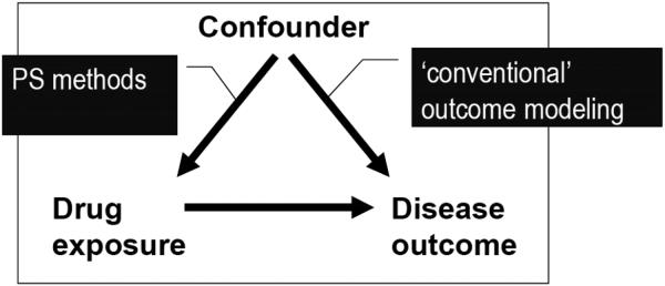
Both arrows need to be present to cause confounding. Removing one of the arrows removes confounding. This leads to essentially two general ways to control for confounding; we can remove the effect of the confounder on treatment (PS methods) or we can condition on the effect of the confounder on the outcome (outcome modeling). Both are dependent on having a good measure of the confounder available to the researcher.

A classic example of confounding (by indication) is the estimation of the effects of beta agonists on asthma mortality. Patients with more severe asthma are more likely to be treated with beta agonists (at any point in time) and asthma severity is an independent predictor of asthma mortality. To depict this confounding by indication using purely hypothetical numbers we have dichotomized the treatment into yes (E=1) or no (E=0) and asthma severity into severe asthma (X=1) and less severe asthma (X=0)(Figure 2).

Figure 2. Numerical Example for Confounding and Uniform Treatment Effects.

The treatment with beta agonists (E) reduces asthma mortality (Y) in both patients with severe (X=1; RR=0.5) and less severe (X=0; RR=0.5) asthma, but the crude relative risk shows that beta agonists are associated with increased mortality (RR=1.74). Note that patients with severe asthma (X=1) are more likely to be treated with beta agonists and more likely to die, which leads to the confounding in the crude (unadjusted) table.

Treatment effect heterogeneity

It is reasonable to assume that treatment effects (both intended and unintended) are not the same in every patient. Good candidates for treatment effect heterogeneity are age (e.g., children and older adults), gender, disease severity, co-morbidity (e.g., diabetes), and comedication (e.g., “polypharmacy”), which are relatively easy to study.

Examples of clinically relevant treatment effect heterogeneity include adjuvant chemotherapy with oxaliplatin in patients with stage III colon cancer, which has been shown to improve survival in patients with a median age of 60 years [21], but may not do so in patients above age 75 years [22], and the primary prevention of myocardial infarction with low-dose aspirin in men [23], but not women [24].

Treatment effect heterogeneity has consequences for the estimation of overall treatment effects. If the effect of treatment with beta agonists is more pronounced in those with severe asthma, the proportion of patients with severe asthma in the study population will influence the estimation of any overall treatment effect (Figure 3). The overall treatment effect in the population will be a weighted average of the treatment effect in those patients with severe asthma and those patients with less severe asthma. The ability to define the population studied (e.g., a population in which the prevalence of severe asthma is 20%) becomes essential, and is a critical component of principled “causal inference”.[25-27] Our focus herein will be on the relative risk (RR). Homogeneous RRs generally imply treatment effect heterogeneity on the risk difference scale if the treatment has an effect and vice versa.

Figure 3. Numerical Example for Confounding and Treatment Effect Heterogeneity.

Hypothetical example of beta agonists and asthma mortality with treatment effect heterogeneity (in addition to confounding, it is possible to construct scenarios without confounding [28], but such a scenario would be implausible for our asthma example); the treatment is not effective in preventing asthma mortality in those with less severe asthma (X=0; RR=1), while being very effective in those with severe asthma (X=1; RR=0.25).

Propensity Scores

Theory

The PS is a covariate summary score defined as the individual probability of treatment (exposure) given (conditional on) all confounders [6]. In our example, 50% of those with severe asthma receive beta agonists, so every patient with severe asthma will have a PS of 0.5 whether or not the patient was actually treated. While in practice there may be different covariate patterns that lead to a PS of 0.5, Rosenbaum and Rubin [6] proved that treated and untreated patients with the same PS value (e.g., treated patients with a PS of 0.5 and untreated patients with a PS of 0.5) will, on average, have the same distribution of covariates used to estimate the PS. Thus, by holding the PS constant (conditioning on the PS) treated and untreated cohorts will tend to be “exchangeable” with respect to the covariates. Exchangeability, in return, leads to unconfounded estimates of treatment effects because it removes the arrow from the covariate(s) to the treatment (Figure 1 above). Note that exchangeability is restricted to measured covariates whose relation with treatment is correctly modeled in the PS. We therefore need to assume no unmeasured confounding, which is much more plausible with randomization, another method to obtain exchangeability.

The ability to control for confounding using PSs is, in general, not different from what we would achieve by using a more conventional multivariable outcome model [8], but the PS has some specific advantages outlined below. The PS also allows us to clearly define the study population in the presence of treatment effect heterogeneity, something that cannot be achieved using a conventional multivariable outcome model [28]. We will now provide a non-technical description of PS estimation and implementation.

Estimation

The PS is usually estimated using multivariable logistic regression. The few published direct comparisons between logistic regression and other methods to estimate the PS (e.g., neural networks [29]; boosted CART [30, 31]) found that PS performs well in most settings. More recently, PS estimation methods based on optimizing balance have been proposed [32]. These are promising, but their performance and causal implications have not yet been thoroughly assessed. It is thus reasonable to use logistic regression to estimate PSs.

As with any model, mis-specification of the PS can lead to bias. An advantage of PSs is that we can check the performance of the model by assessing covariate balance across treatment groups after stratifying, matching, or weighting on the estimated PS (PS implementation discussed below). If covariate imbalances remain, the PS model can be refined, e.g., by using less restrictive terms for continuous covariates (e.g., squared or cubic terms, fractional polynomials, and splines) or by adding interaction terms between covariates.

Although the ability to check covariate balance is a beneficial aspect of PS methods, there is no agreed-upon best way to check or summarize covariate balance. The vast majority of the current methods proposed to quantify covariate imbalances do not take the confounding potential of the remaining imbalances into account. We therefore suggest using the approach proposed by Lunt et al. [33] that assesses the confounding potential of remaining imbalances by assessing the change in estimate after controlling for individual covariates in the outcome model after PS implementation. A change in estimate indicates a remaining imbalance of the covariate across treatment groups and that the covariate affects the risk for the outcome independent of treatment. A graphical depiction of the spread of the changes in estimate can then be used to compare different PS estimation or implementation methods [33].

As in any non-experimental study, the process of variable selection is also important for PS models. The crux lies in the inability of the data to inform us about causal structures. In fact, data cannot be analyzed without the researcher imposing a causal structure [34].

Thus far we have depicted the PS as a model predicting treatment based on covariates. We now need to add an important distinction between the PS and a model intended to optimize discrimination between treatment groups.[35] Consider in our hypothetical study of beta agonists outlined above a random selection of the physicians treating patients with asthma has recently been visited by a detailer making a very compelling argument to treat more patients with beta agonists irrespective of asthma severity. So, we build the PS based on asthma severity (and all potential risk factors for asthma mortality, the outcome of interest) to control for confounding. Should we add the variable “recent detailer visit” to the PS model? Because the detailer visit leads to increased prescribing irrespective of asthma severity, it will clearly improve our prediction of treatment with beta agonists, but does this help with respect to our aim (i.e., to estimate the unconfounded effect of beta agonists on asthma mortality)? The answer is no, and even worse, to the contrary. Having had a detailer visit is an “instrumental variable,” i.e., a variable associated with the treatment of interest, but not affecting the outcome (asthma mortality) other than through its relation with the treatment (beta agonists).

In medical research, instrumental variables are those that explain variation in treatments, but are not directly related to the outcome of interest. As outlined above, this is the “good” variability (e.g., the change in prescribing following the detailer visit). Without such variability, we would not be able to conduct non-experimental research. By removing “good” variability, we not only decrease the precision of the estimate [36], but also increase the contribution of “bad” variability, i.e., unaccounted for variability in treatments that affects the risk for the outcome (also called unmeasured confounding) [16, 37]. This issue is not just academic [38] and the crux lies in the fact that the data will not tell us whether or not a variable is a confounder or an instrumental variable. Some have argued that it is safer to err on the side of including variables in the PS [37] or to use automated procedures to screen hundreds of potential covariates in studies using large automated healthcare databases [39]. Automated procedures have been shown to improve confounding control in some [39], but not all settings [40, 41]. They should be implemented with care and considering the potential for inclusion of instrumental variables.

Implementation

Once the PS is estimated, we can control for this covariate summary score as for any other continuous covariate using standard epidemiologic techniques, including stratification, matching, standardization (weighting), and outcome regression modeling. Modeling (adding the PS to a multivariable outcome model) is the least appealing of these implementation methods because its validity is dependent on correctly specifying two models (the PS and the outcome model) and it also does not offer specific advantages of other PS implementations, as outlined below. We therefore do not recommend implementing the PS as a continuous covariate in an outcome regression model.

One of the main advantages of the PS is that it provides an easy way to check whether or not there are some patient characteristics (covariate patterns) that define groups of patients in whom there is no variability in treatments (i.e., everyone treated or no one treated;Figure 4). It might be that, following our beta agonists and asthma example, within the group of patients with mild asthma there is a group of patients with very mild asthma in which no one is treated with beta agonists. It is easy to see that there are no data to estimate any treatment effect in this group, unless we make the strong, and likely incorrect assumption that risk of death and treatment effects in these patients with very mild would be identical to those in the group of treated patients with mild asthma. While extrapolation of treatment effects to groups for whom we have no data to estimate the treatment effect may be very sensible in practice, researchers should at least be aware of such extrapolations. PSs allow us to limit model extrapolation by excluding patient groups from the analysis in whom no treatment effect can be estimated because all patients are either never (untreated with PS lower than the lowest PS in the treated) or always treated (treated with higher PS than the highest PS in the untreated). Trimming (excluding) non-overlap regions of PS should be the default prior to any PS implementation. The untrimmed and trimmed populations need to be compared; however, because trimming patients with very mild asthma (our example) leads to a focused inference that is not generalizable to all asthmatics.

Figure 4.

Schematic for Non-Overlap in Propensity Score Distributions – Exclusion (Trimming) of Non-Overlap (Shaded Areas) Reduces Model Extrapolation to Covariate Patterns in Which No Treatment Comparison Can Be Made (“Non-Positivity”)

Stratification of continuous covariates into equal-sized strata (percentiles), estimation of the treatment effect within these percentiles, and combining the stratum-specific estimates using a weighted average (e.g., Mantel-Haenszel; MH [42]) is a well-established method to control for confounding by any continuous covariate, including the PS. Trimming of non-overlap should be done before creating percentiles. Depending on the number and distribution of outcomes, it is often possible to use 10 strata (deciles) rather than the “usual” five strata (quintiles), thus reducing residual confounding within strata. Because most methods to average stratum-specific estimates assume uniform treatment effects across strata, it is important to estimate and evaluate the stratum-specific treatment effect estimates before combining the stratum-specific treatment effect estimates into an overall estimate. Using our numerical example above (Figure 2), stratifying on the PS will be the same as stratifying on asthma severity; there are only two distinct PS values (PS=0.5 for all those with X=1 and PS=0.1 for all those with X=0). Because the treatment effect is uniform (RR=0.5 in both PS strata) we know that any weighted average, including the MH estimate, of the unconfounded effect of beta agonists on asthma mortality in our cohort will yield a RR=0.5.

Matching on specific covariates in cohort studies removes confounding by the matching variable(s) and has been used extensively in epidemiologic research prior to the widespread availability of multivariable models [43]. Matching on a large number of covariates quickly becomes intractable; however, and summary scores, including the PS, were originally proposed to overcome this limitation [44, 45]. In theory, the implementation is straightforward; for every treated patient we find a single or multiple untreated patients with the same PS (or nearly the same PS, based on a pre-determined caliper) and put the matched pair aside. We then repeat this step until we acquire all of the treated patients matched to the same number of untreated patients (a selection of all the untreated patients). In practice, however, this is more complicated because we may not find an untreated match for every treated patient. The ability to find matches for all treated patients is a complex function of the overall prevalence of the treatment in the population, the separation of the PS distribution in treated and untreated patients, and the width of the PS caliper used [33, 46]. There is a general trade-off between residual confounding (minimized by narrow calipers) and finding matches (maximized by wide calipers). Various matching algorithms are available and the comparative performance has been assessed using simulations [47]. We have often used a greedy matching algorithm [48] and this has been shown to perform well in both actual studies and simulations [47]. It is important to report the number or proportion of treated patients that could be matched. Higher proportions are preferred. Note that the proportion of untreated patients that could be matched, and therefore the overall number of patients matched, is not relevant here.

Standardization is a way to validly summarize treatment effects in the presence of treatment effect heterogeneity. Note that matching implicitly standardizes the estimate to the treated population. “Standardizing” to the treated population can also be achieved using standardized mortality/morbidity ratio (SMR) weights [49] (the quotes around “standardizing” are due to a technicality: we can only standardize on categories of variables, whereas weighting actually allows us to include continuous variables and is thus more flexible). These weights create a pseudo-population of the untreated, which has the same covariate distribution as the treated. While every treated person receives a weight of 1 (i.e., the observed), every untreated person is weighted by the PS odds [PS/(1-PS)]:

$$\text{SMR W}=\mathrm{E}+{(1-\mathrm{E})}^{\ast }\left(\text{PS}\right)∕(1-\text{PS})$$

We now use our numerical examples presented in Figures 2 and 3 to illustrate PS implementation to estimate the average treatment effect in the treated. For clarity, we retain the single, dichotomous covariate example in which there is no difference between controlling for this single covariate and the PS. In practice, however, the PS will be a summary score of multiple covariates reduced into a single covariate, which allows us to efficiently implement all that follows rather than doing this for each and every covariate separately. PS matching (in expectation) and SMR weighting will lead to the numbers presented in Figure 5 and an unconfounded RR=0.5 in the collapsed table. The prevalence of treatment, and thus the estimated PS, is 0.1 in those with X=0 and 0.5 in those with X=1.

Figure 5. Numerical Example for PS Matching and SMR Weighting.

We present the SMR weights (w) separately for all exposure (E) and covariate (X) patterns; in a real study, they would be calculated based on exposure status and the estimated PS. Note that in our numerical example we can match all those treated and for matching and SMR weighting, the prevalence of severe asthma (X=1) in the untreated (1000/1800=0.55) is the same as the prevalence of severe asthma in the treated (1000/1800 – see Figure 2). The fact that the size of the study population is reduced only affects the precision of the estimate, but not its validity nor its causal interpretation.

Another typical standard is the overall population of the treated and untreated. This can be achieved by implementing the PS using inverse probability of treatment weights (IPTW). In settings with an active comparator, estimating the treatment effect in the entire population obviates the need to determine which treatment to identify as treated and untreated in PS matching and SMR weighting. IPTW creates a pseudo-population of both the treated and the untreated, which has the same covariate distribution as the overall population of treated and untreated. Every person is weighted by the inverse of the probability of receiving the treatment actually received [the PS in the treated and (1-PS) in the untreated]. Stabilizing these weights by the marginal overall prevalence of the treatment actually received has specific advantages that are beyond the scope of this review.[27] The actual stabilized IPTW weights are easily implemented based on the estimated PS, as follows:

$${\text{IPTW W}}_{\text{Stabilized}}={\mathrm{E}}^{\ast }{\mathrm{P}}_{\mathrm{E}}∕\text{PS}+{(1-\mathrm{E})}^{\ast }(1-{\mathrm{P}}_{\mathrm{E}})∕(1-\text{PS}),\text{where}{\mathrm{P}}_{\mathrm{E}}\text{is the overall marginal prevalence of the treatment exposure}$$

In our numerical example, the marginal prevalence of treatment, P_E, is 0.18 (Figure 2). Using our estimated PS values would lead to the weights, and on average, the numbers presented in Figure 6 and again to an unconfounded RR=0.5 in the collapsed table.

Figure 6. Numerical Example for Inverse Probability of Treatment Weighting.

All observed N and numbers of events (Y=1) in Figure 2 are multiplied by the (stabilized) IPTW weights leading to the pseudo-populations depicted in the stratified tables above, which are then collapsed into the table on the right without matching. Note that those treated contrary to prediction (E=1 when X=0) are up-weighted (weight > 1), while those treated according to prediction (E=0 when X=0 and E=1 when X=1) are down-weighted to achieve covariate balance across treatment groups. The distribution of severe asthma (X=1) in treated and untreated is now the same as in the total population (prevalence of 20%; Figure 2).

In our above numerical example, all PS implementation methods led to the same unconfounded treatment effect estimate (RR=0.5) because the treatment effect is uniform. The results for our numerical example with heterogeneous treatment effects, as introduced in Figure 3, are shown below in Figure 7. As can be seen, the treatment effect in the treated (PS matching or SMR) is more pronounced than the treatment effect in the population (IPTW). Note that all estimates are unconfounded. The difference between the estimates from MH, PS matching or SMR, and IPTW is due to the fact that the prevalence of severe asthma, in which the treatment is effective, is higher in treated patients (55%) than the entire population of treated and untreated (20%). The MH estimate is not valid in this setting because it assumes uniform effects and the MH weighted average does not pertain to any defined population; the weights are entirely chosen to minimize variance and result in relying heavily on the stratum with severe asthma (X=1) because most of the events are observed in this stratum (w=0.93).

Figure 7.

Numerical Example for Mantel Haenszel (Invalid, for Comparison Only), Standardized Mortality/Morbidity Ratio (SMR), PS Matching, and SMR Weighting, and Inverse Probability of Treatment Weighting in the Presence of Treatment Effect Heterogeneity

PS matching, the SMR, and IPTW result in so-called causal contrasts because the population of interest is clearly defined. The data (Figs. 3, 7) suggest that there is no value to use of beta agonists in those with mild asthma (X=0). With such marked heterogeneity, presenting treatment effects stratified by asthma severity would be essential and any average treatment effect would have uncertain utility for treatment decisions in practice.[50]

PS matching and SMR weights allow us to estimate the average treatment effect in the treated, i.e., in patients with the same distribution of covariates as the one actually observed in the treated. The average treatment effect in the treated answers the question, “What would have happened if those actually treated had not received treatment?” In our experience, matching or SMR weighting are preferable when the comparator group is either untreated or not well-defined, as is often the case in pharmacoepidemiology (although active referent groups are increasingly used in settings, such as evaluation of comparative effectiveness). Estimating the treatment effect in a population with a reasonably high prevalence of the indication for treatment reduces the potential for violations of positivity that we would likely encounter with IPTW in such a setting.

With an active comparator (a treatment alternative rather than untreated), the indication can often be assumed to be equally prevalent in both treatment groups, thus limiting the potential for violations of positivity. IPTW will often make sense with an active comparator, allowing us to estimate the average treatment effect in the entire population. This answers the question of what would have happened if everyone had been treated with “A” versus what would have happened if everyone had been treated with “B,” the same question that is asked in an RCT [51]. Note that being able to make these causal contrasts is dependent on predicting treatment based on relevant covariates, i.e., the estimation of the PS [6].

In practice, the distribution of weights needs to be carefully checked for both SMR weighting and IPTW because some patients, i.e., those treated contrary to prediction, receive large weights (are “replicated” or “cloned” many times), and thus can become highly influential. For IPTW a rule of thumb for well-behaved weights (“no problem”) would be a mean stabilized weight close to 1.0 and a maximum stabilized weight of < 10 [52]. Thus far, no similar rule of thumb has been evaluated for SMR weighting, but in the meantime it would seem reasonable to also use weights ≥ 10 as a sign for concern. If weights > 10 are observed, researchers should check whether or not instrumental variables can be excluded from the PS model and perform sensitivity analyses involving additional trimming (see below).

Trimming

Thus far we have assumed no unmeasured confounding. While this assumption is necessary to estimate treatment effects using any adjustment method, in reality the assumption of no unmeasured confounding will often be violated to some extent. Some patients that have the indication for treatment (e.g., because they have severe asthma) may be too frail to receive the treatment. Because frailty is a concept that is difficult to measure, it can lead to substantial bias in non-experimental studies of medical interventions compared with no intervention [19, 53]. Because the PS focuses on treatment decisions, it allows us to identify patients treated contrary to prediction in whom confounding, e.g., by frailty, may be most pronounced. These are the untreated patients with the highest PS and the treated patients with the lowest PS (Figure 8). Under this assumption, trimming increasing proportions of those at both ends of the overlapping PS distribution has been shown to reduce unmeasured confounding [14]. It is important to use a percentage (e.g., 1%, 2.5%, and 5%) of those treated contrary to prediction to derive cut-points for trimming only. Once these cut-point have been established, both treated and untreated below the lower and above the higher cut-points need to be excluded from the analysis to avoid introducing bias. The choice of cut-points will depend on the specific setting and the change in the treatment effect estimate across various cut-points will be more informative than any specific value, and thus results from the whole range of trimming should be reported (in addition to the number of patients and events trimmed by treatment group). According to our experience, trimming may be especially important with IPTW, but we recommend routinely performing a sensitivity analysis based on trimming for any PS implementation method. As with any sensitivity analysis, transparency is important and untrimmed results need to always be presented together with trimmed results. As with trimming non-overlap, as described above, additional trimming within the overlap population leads to a more focused inference that is no longer generalizable to the treated or the entire population.

Figure 8.

Schematic for Trimming at the Ends of the (Overlapping) Propensity Score Distribution

Recommendations

PSs are an alternative to multivariable outcome models to control for measured confounding. Compared with multivariable outcome models, PSs have specific advantages, including identification of barriers for treatment (e.g., older adults), the implicit consideration of relative timing of covariates and treatment (covariate should precede treatment initiation), the ability to present the resulting balance of covariates which is needed to remove confounding (exchangeability), the trimming of patients outside of a common range of covariates in whom we have no data to estimate the treatment effect, the ability to estimate causal contrasts in the presence of treatment effect heterogeneity, and the ability to control for many covariates in settings with many treated and rare outcomes.[11] We have focused on causal contrasts in the presence of heterogeneous treatment effects because we think that this issue is not well-recognized by clinical researchers. Treatment effects are likely to be heterogeneous across age, gender, co-morbidities, and co-medications, and PSs as implemented using matching or weighting allow us to estimate valid overall treatment effects in such settings. With strong treatment effect heterogeneity across the PS, research should attempt to pinpoint actual covariates leading to heterogeneity because identification of such patient groups might be relevant for clinical practice. For example, the data in Figures 3 and 7 raise the possibility that treatment has no benefit in those with X=0, but has an even greater benefit in those with X=1 than the estimated overall treatment effect. This might spur further evaluation of subgroup-specific effects and consideration of shifts in the population targeted for treatment. With an unexposed comparison group, estimating the treatment effect in the treated (PS matching or SMR weighting) will often be preferred because we would rarely want to treat everyone who is currently not treated. In the setting of an active comparator (e.g., comparative effectiveness research), estimating the treatment effect in the entire population (IPTW) will often make most sense because we are focusing on treatment choice after the treatment decision per se has been made. Heterogeneous treatment effects can also be due to unmeasured confounding concentrated in those treated contrary to prediction. Sensitivity analyses based on PSs allow us to assess the potential for and reduce such unmeasured confounding.

References

- 1.Concato J, Shah N, Horwitz RI. Randomized, controlled trials, observational studies, and the hierarchy of research designs. N Engl J Med. 2000;342:1887–1892. doi: 10.1056/NEJM200006223422507. [DOI] [PMC free article] [PubMed] [Google Scholar]
- 2.Miettinen OS. The need for randomization in the study of intended drug effects. Stat Med. 1983;2:267–271. doi: 10.1002/sim.4780020222. [DOI] [PubMed] [Google Scholar]
- 3.Yusuf A, Collins R, Peto R. Why do we need some large, simple randomized trials? Stat Med. 1984;3:409–420. doi: 10.1002/sim.4780030421. [DOI] [PubMed] [Google Scholar]
- 4.Prentice RL, Langer R, Stefanick ML, et al. Combined Postmenopausal Hormone Therapy and Cardiovascular Disease: Toward Resolving the Discrepancy between Observational Studies and the Women’s Health Initiative Clinical Trial. Am J Epidemiol. 2005;162(5):404–14. doi: 10.1093/aje/kwi223. [DOI] [PubMed] [Google Scholar]
- 5.Walker AM. Confounding by indication. Epidemiology. 1996;7:335–336. [PubMed] [Google Scholar]
- 6.Rosenbaum PR, Rubin DB. The central role of the propensity score in observational studies for causal effects. Biometrika. 1983;70:41–55. [Google Scholar]
- 7.Stürmer T, Joshi M, Glynn RJ, Avorn J, Rothman KJ, Schneeweiss S. A review of the application of propensity score methods yielded increasing use, advantages in specific settings, but not substantially different estimates compared with conventional multivariable methods. J Clin Epidemiol. 2006;59:437–47. doi: 10.1016/j.jclinepi.2005.07.004. [DOI] [PMC free article] [PubMed] [Google Scholar]
- 8.Stürmer T, Schneeweiss S, Brookhart MA, Rothman KJ, Avorn J, Glynn RJ. Analytic Strategies to adjust confounding using Exposure Propensity Scores and Disease Risk Scores: Nonsteroidal Antiinflammatory Drugs (NSAID) and Short-Term Mortality in the Elderly. Am J Epidemiol. 2005;161:891–8. doi: 10.1093/aje/kwi106. [DOI] [PMC free article] [PubMed] [Google Scholar]
- 9.Rubin DB. The design versus the analysis of observational studies for causal effects: parallels with the design of randomized trials. Stat Med. 2007;26:20–36. doi: 10.1002/sim.2739. [DOI] [PubMed] [Google Scholar]
- 10.Ray WA. Evaluating Medication Effects Outside of Clinical Trials: New-User Designs. Am J Epidemiol. 2003;158:915–920. doi: 10.1093/aje/kwg231. [DOI] [PubMed] [Google Scholar]
- 11.Glynn RJ, Schneeweiss S, Stürmer T. Indications for propensity scores and review of their use in pharmacoepidemiology. Basic Clin Pharmacol Toxicol. 2006;98:253–259. doi: 10.1111/j.1742-7843.2006.pto_293.x. [DOI] [PMC free article] [PubMed] [Google Scholar]
- 12.Messer LC, Oakes JM, Mason S. Effects of socioeconomic and racial residential segregation on preterm birth: a cautionary tale of structural confounding. Am J Epidemiol. 2010;171:664–673. doi: 10.1093/aje/kwp435. [DOI] [PubMed] [Google Scholar]
- 13.Westreich D, Cole SR. Invited commentary: positivity in practice. [Commentary] Am J Epidemiol. 2010;171:674–677. doi: 10.1093/aje/kwp436. [DOI] [PMC free article] [PubMed] [Google Scholar]
- 14.Stürmer T, Rothman KJ, Avorn J, Glynn RJ. Treatment effects in the presence of unmeasured confounding: Dealing with observations in the tails of the propensity score distribution – a simulation study. Am J Epidemiol. 2010 doi: 10.1093/aje/kwq198. doi: 10.1093/aje/kwq198. [DOI] [PMC free article] [PubMed] [Google Scholar]
- 15.Hernán MA, Alonso A, Logan R, Grodstein F, Michels KB, Willett WC, Manson JE, Robins JM. Observational studies analyzed like randomized experiments: an application to postmenopausal hormone therapy and coronary heart disease. Epidemiology. 2008;19:766–779. doi: 10.1097/EDE.0b013e3181875e61. [DOI] [PMC free article] [PubMed] [Google Scholar]
- 16.Brookhart MA, Stürmer T, Glynn RJ, Rassen J, Schneeweiss S. Confounding control in healthcare database research: challenges and potential approaches. Medical Care. 2010;48(Suppl 1):S114–20. doi: 10.1097/MLR.0b013e3181dbebe3. [DOI] [PMC free article] [PubMed] [Google Scholar]
- 17.Sackett DL, et al. Evidence-based medicine : how to practice and teach EBM. Churchill Livingstone; New York: 1997. [Google Scholar]
- 18.Redelmeier DA, Tan SH, Booth GL. The treatment of unrelated disorders in patients with chronic medical diseases. N Engl J Med. 1998;338(21):1516–1520. doi: 10.1056/NEJM199805213382106. [DOI] [PubMed] [Google Scholar]
- 19.Glynn RJ, Knight EL, Levin R, Avorn J. Paradoxical relations of drug treatment with mortality in older persons. Epidemiology. 2001;12(6):682–689. doi: 10.1097/00001648-200111000-00017. [DOI] [PubMed] [Google Scholar]
- 20.Rothman KJ, Greenland S, Lash TL. Modern Epidemiology. 3rd Lippincott Williams & Wilkins; Philadelphia: 2008. [Google Scholar]
- 21.André T, Boni C, Mounedji-Boudiaf L, et al. Oxaliplatin, fluorouracil, and leucovorin as adjuvant treatment for colon cancer. N Engl J Med. 2004;350:2343–51. doi: 10.1056/NEJMoa032709. [DOI] [PubMed] [Google Scholar]
- 22.Sanoff HK, Carpenter WR, Stürmer T, Goldberg RM, Martin CF, Fine JP, McCleary NJ, Meyerhardt JA, Niland J, Kahn KL, Schymura MJ, Schrag D. The Effect of Adjuvant Chemotherapy on Survival of Patients with Stage III Colon Cancer Diagnosed After Age 75. Journal of Clinical Oncology J Clin Oncol. 2012;30(21):2624–34. doi: 10.1200/JCO.2011.41.1140. [DOI] [PMC free article] [PubMed] [Google Scholar]
- 23.Steering Committee of the Physicians’ Health Study Research Group. Final report on the aspirin component of the ongoing Physicians’ Health Study. N Engl J Med. 1989;321:129–35. doi: 10.1056/NEJM198907203210301. [DOI] [PubMed] [Google Scholar]
- 24.Ridker PM, Cook NR, Lee IM, Gordon D, Gaziano JM, Manson JE, Hennekens CH, Buring JE. A randomized trial of low-dose aspirin in the primary prevention of cardiovascular disease in women. N Engl J Med. 2005;352(13):1293–304. doi: 10.1056/NEJMoa050613. [DOI] [PubMed] [Google Scholar]
- 25.Pearl J. Causality: Models, Reasoning, and Inference. Cambridge University Press; New York, NY: 2000. [Google Scholar]
- 26.Robins JM, Hernán MA, Brumback B. Marginal structural models and causal inference in epidemiology. Epidemiology. 2000;11(5):550–60. doi: 10.1097/00001648-200009000-00011. [DOI] [PubMed] [Google Scholar]
- 27.Hernán MA, Brumback B, Robins JM. Marginal structural models to estimate the causal effect of zidovudine on the survival of HIV-positive men. Epidemiology. 2000;11:561–570. doi: 10.1097/00001648-200009000-00012. [DOI] [PubMed] [Google Scholar]
- 28.Stürmer T, Rothman KJ, Glynn RJ. Insights into different results from different causal contrasts in the presence of effect-measure modification. Pharmacoepidemiol Drug Saf. 2006;15:698–709. doi: 10.1002/pds.1231. [DOI] [PMC free article] [PubMed] [Google Scholar]
- 29.Setoguchi S, Schneeweiss S, Brookhart M, Glynn R, Cook E. Evaluating uses of data mining techniques in propensity score estimation: a simulation study. Pharmacoepidemiol Drug Saf. 2008;17(6):546–55. doi: 10.1002/pds.1555. [DOI] [PMC free article] [PubMed] [Google Scholar]
- 30.Lee B, Lessler J, Stuart E. Improving propensity score weighting using machine learning. Statist Med. 2010;29(3):337–46. doi: 10.1002/sim.3782. [DOI] [PMC free article] [PubMed] [Google Scholar]
- 31.Ellis AR, Dusetzina SB, Hansen RA, Gaynes BN, Farley JF, Stürmer T. Propensity Scores from Logistic Regression Yielded Better Covariate Balance Than Those from a Boosted Model: A Demonstration Using STAR*D Data. Pharmacoepidemiol Drug Saf. 2011;20:S129. [Google Scholar]
- 32.Imai K, Ratkovic M. Covariate balancing propensity score. 2012 Working paper available at http://imai.princeton.edu/research/CBPS.html. [Google Scholar]
- 33.Lunt M, Solomon DH, Rothman KJ, Glynn RJ, Hyrich K, Symmons DPM, Stürmer T. Different Methods of Balancing Covariates Leading to Different Effect Estimates in the Presence of Effect Modification. American Journal of Epidemiology. 2009;169:909–17. doi: 10.1093/aje/kwn391. [DOI] [PMC free article] [PubMed] [Google Scholar]
- 34.Robins JM. Data, Design, and Background Knowledge in Etiologic Inference. Epidemiology. 2001;12(3):313–20. doi: 10.1097/00001648-200105000-00011. [DOI] [PubMed] [Google Scholar]
- 35.Westreich D, Cole SR, Jonsson Funk M, Brookhart MA, Stürmer T. The role of the c-statistic in variable selection for propensity score models. Pharmacoepidemiology and Drug Safety. 2011;20(3):317–20. doi: 10.1002/pds.2074. [DOI] [PMC free article] [PubMed] [Google Scholar]
- 36.Brookhart MA, Schneeweiss S, Rothman KJ, Glynn RJ, Avorn J, Stürmer T. Variable selection in propensity score models: some insights from a simulation study. American Journal of Epidemiology. 2006;163:1149–56. doi: 10.1093/aje/kwj149. [DOI] [PMC free article] [PubMed] [Google Scholar]
- 37.Myers JA, Rassen JA, Gagne JJ, Huybrechts KF, Schneeweiss S, Rothman KJ, Joffe MM, Glynn RJ. Effects of adjusting for instrumental variables on bias and precision of effect estimates. Am J Epidemiol. 2011 Dec 1;174(11):1213–22. doi: 10.1093/aje/kwr364. [DOI] [PMC free article] [PubMed] [Google Scholar]
- 38.Patrick AR, Schneeweiss S, Brookhart MA, Glynn RJ, Rothman K, Avorn J, Stürmer T. The implications of propensity score variable selection strategies in pharmacoepidemiology – an empirical illustration. Pharmacoepidemiology and Drug Safety Mar. 2011;20(6):551–559. doi: 10.1002/pds.2098. [DOI] [PMC free article] [PubMed] [Google Scholar]
- 39.Schneeweiss S, Rassen JA, Glynn RJ, Avorn J, Mogun H, Brookhart MA. High-dimensional propensity score adjustment in studies of treatment effects using health care claims data. Epidemiology. 2009 Jul;20(4):512–22. doi: 10.1097/EDE.0b013e3181a663cc. [DOI] [PMC free article] [PubMed] [Google Scholar]
- 40.Rassen JA, Glynn RJ, Brookhart MA, Schneeweiss S. Covariate selection in high-dimensional propensity score analyses of treatment effects in small samples. Am J Epidemiol. 2011;173(12):1404–13. doi: 10.1093/aje/kwr001. [DOI] [PMC free article] [PubMed] [Google Scholar]
- 41.Toh S, García Rodríguez LA, Hernán MA. Confounding adjustment via a semi-automated high-dimensional propensity score algorithm: an application to electronic medical records. Pharmacoepidemiol Drug Saf. 2011;20(8):849–57. doi: 10.1002/pds.2152. [DOI] [PMC free article] [PubMed] [Google Scholar]
- 42.Mantel N, Haenszel W. Statistical aspects of the analysis of data from retrospective studies of disease. J Natl Cancer Inst. 1959 Apr;22(4):719–48. [PubMed] [Google Scholar]
- 43.Stürmer T, Poole C. Matching in cohort studies: return of a long lost family member. American Journal of Epidemiology. 2009;169(Suppl):S128. [Google Scholar]; Symposium. 42nd annual meeting of the Society for Epidemiologic Research, Anaheim,; 2009. [DOI] [PubMed] [Google Scholar]
- 44.Peters CC. A Method of Matching Groups for Experiment with No Loss of Population. The Journal of Educational Research. 1941;34(8):606–612. [Google Scholar]
- 45.Belson WA. Matching and Prediction on the Principle of Biological Classification. Journal of the Royal Statistical Society. Series C (Applied Statistics) 1959;8(2):65–75. [Google Scholar]
- 46.Ellis AR, Dusetzina SB, Hansen RA, Gaynes BN, Farley JF, Stürmer T. Investigating differences in treatment effect estimates between propensity score matching and weighting: A demonstration using STAR*D trial data. Pharmacoepidemiology and Drug Safety. PDS-12-0105.R2. [DOI] [PMC free article] [PubMed]
- 47.Austin PC. Some methods of propensity-score matching had superior performance to others: results of an empirical investigation and Monte Carlo simulations. Biom J. 2009 Feb;51(1):171–84. doi: 10.1002/bimj.200810488. [DOI] [PubMed] [Google Scholar]
- 48.Parsons LS. Reducing bias in a propensity score matched-pair sample using greedy matching techniques, 2001 ( http://www2.sas.com/proceedings/sugi26/p214-26.pdf) [Google Scholar]
- 49.Sato T, Matsuyama Y. Marginal structural models as a tool for standardization. Epidemiology. 2003 Nov;14(6):680–6. doi: 10.1097/01.EDE.0000081989.82616.7d. [DOI] [PubMed] [Google Scholar]
- 50.Kurth T, Walker AM, Glynn RJ, Chan KA, Gaziano JM, Berger K, Robins JM. Results of multivariable logistic regression, propensity matching, propensity adjustment, and propensity-based weighting under conditions of nonuniform effect. Am J Epidemiol. 2006;163(3):262–70. doi: 10.1093/aje/kwj047. [DOI] [PubMed] [Google Scholar]
- 51.Hernán MA. A definition of causal effect for epidemiological research. J Epidemiol Community Health. 2004;58(4):265–71. doi: 10.1136/jech.2002.006361. [DOI] [PMC free article] [PubMed] [Google Scholar]
- 52.Cole SR, Hernán MA. Constructing inverse probability weights for marginal structural models. Am J Epidemiol. 2008 Sep 15;168(6):656–64. doi: 10.1093/aje/kwn164. [DOI] [PMC free article] [PubMed] [Google Scholar]
- 53.Jackson LA, Jackson ML, Nelson JC, Neuzil KM, Weiss NS. Evidence of bias in estimates of influenza vaccine effectiveness in seniors. Int J Epidemiol. 2006;35:337–44. doi: 10.1093/ije/dyi274. [DOI] [PubMed] [Google Scholar]