Abstract
We sequenced 114 genes (for DNA repair, cell cycle arrest, apoptosis, and detoxification)in a mixed human population and observed a sudden increase in the number of functional polymorphisms below a minor allele frequency of ∼6%. Functionality is assessed by considering the ratio in the number of nonsynonymous single nucletide polymorphisms (SNPs)to the number of synonymous or intron SNPs. This ratio is steady from below 1% in frequency—that regime traditionally associated with rare Mendelian diseases—all the way up to about 6% in frequency, after which it falls precipitously. We consider possible explanations for this threshold effect. There are four candidates as follows: (1)deleterious variants that have yet to be purified from the population, (2)balancing selection, in which a selective advantage accrues to the heterozygotes, (3)population-specific functional polymorphisms, and (4)adaptive variants that are accumulating in the population as a response to the dramatic environmental changes of the last 7,000∼17,000 years.
The prevailing view in human genetics is that most polymorphisms are selectively neutral (Kimura 1983). In contrast, the ultimate objective of research on the genetic basis of disease is the identification of functional polymorphisms that determine phenotype. As a practical matter, only a miniscule fraction of the extant polymorphisms could plausibly influence cellular function. This is because <2% of the human genome codes for protein, and only 5% is under selection, on the basis of comparison with the recently sequenced mouse genome (Waterston et al. 2002). Few large-scale polymorphism discovery efforts have focused on this 2%∼5% of the genome, and even fewer have searched deep enough to identify polymorphisms that occur infrequently in the population. To the extent that it has been done, subtle anomalies in the polymorphism distribution at low frequencies (Cargill et al. 1999; Halushka et al. 1999; Stephens et al. 2001) were attributed to differing forms of selection (Harpending and Rogers 2000; Przeworski et al. 2000; Fay et al. 2001). We examine, in greater detail, one of these low frequency anomalies on a set of genes chosen for their high likelihood of importance to disease.
Before proceeding, we must clarify the use of the word functional in the context of the single nucleotide polymorphisms (SNPs) that are the focus of our work. Functional SNPs can be located anywhere. We define four categories. SNPs found in the protein-coding regions are either nonsynonymous or synonymous, depending on whether they do or do not change the protein sequence. SNPs found in the nonprotein-coding regions are either intron or intergenic. The essential point is that a randomly chosen nonsynonymous SNP is more likely to be functional than a randomly chosen synonymous, intron, or intergenic SNP. This assertion is supported by the observed frequencies of occurrence in the human population for the different SNP categories. Nonsynonymous SNPs tend to be found less frequently, given the availability of sites. In the analysis to be presented, synonymous and intron SNPs both behave as expected by neutral theory. This does not imply that they are never functional, only that an extremely small fraction of them are functional, hence, to a first approximation, either can be used to establish a neutral theory baseline to normalize out the complexities of population history. Given the lower quality of our intron data, we focus on the NON/SYN ratio for the number of nonsynonymous to synonymous SNPs. Under neutral theory, this ratio is expected to be constant as a function of the minor allele frequency. The fact that it is not is the main point of interest.
Cargill et al. (1999) reported NON/SYN ratios of 1.20, 0.72, and 0.61 in the frequency ranges of 0%–5%, 5%–15%, and 15%–50%, respectively. This result was based on 392 coding SNPs, in 106 genes that are related to cardiovascular disease, endocrinology, and neuropsychiatry. On average, 57 diploid individuals were sampled from a mixed population. Cargill et al. (1999) explained this phenomenon by positing a background of deleterious variants in mutation-selection balance. Beside wanting to replicate this result in another set of disease-related genes, we wanted to examine the shape of this frequency dependence. After all, with only three data points, one can never be sure. The simplest assumption is a ski-slope shape, but the reality is surprisingly different, as we discovered by dissecting the frequency axis in a way that maximizes the signal-to-noise ratio.
RESULTS
A total of 114 genes were resequenced under the Environmental Genome Project, with a focus on genes that are implicated in DNA repair, cell cycle arrest, apoptosis, and detoxification. The entire list is at http://www.genome.washington.edu/projects/egpsnps. Polymorphisms were identified by direct resequencing of PCR amplicons from a mixed population, the NHGRI/Coriell Human Diversity Panel (Collins et al. 1998), abbreviated HDP. A total of 64, 38, and 12 genes were sampled at depths of 44, 90, and 450 diploid individuals, respectively. Averaged across this gene set, each base was sampled at a mean depth of 83.6 diploid individuals. The total length of the resequenced coding exons was 191.5 Kb, and another 207.4 Kb of the flanking introns was resequenced in the process. Every analyzed gene was autosomal. We identified 616 coding SNPs, of which, 337 were nonsynonymous and 279 were synonymous. There were also 663 intron SNPs. The nonsynonymous SNPs included five conversions to a stop codon, all at a minor allele frequency of 0.0139 or less, and three of these converted to UGA, which may code for selenocysteine instead of a stop. There were two frame-shift mutations, but only in a single heterozygous individual, and at the extreme sample depth of 450.
For comparison with the published data, we correct for variations in sample depth and sequence length by estimating the mutation parameter θ, along the lines of Cargill et al. (1999). Suppose K polymorphic sites are identified by sequencing n chromosomes in a region of length L. The desired estimate is
 |
Summed across the genes, we find that θ(NON) = 3.23 × 10⁻⁴, θ(SYN) = 2.67 × 10⁻⁴, and θ(INT) = 5.89 × 10⁻⁴, for nonsynonymous, synonymous, and intron SNPs, respectively. When we further adjust for the fact that there is a 0.775 probability of any substitution in the coding region of our specific genes to be nonsynonymous, we find that θ(NON) = 4.17 × 10⁻⁴ and θ(SYN) = 11.9 × 10⁻⁴. These numbers are in good agreement with Cargill et al. (1999) θ(NON) = 3.59 × 10⁻⁴ and θ(SYN) = 10.0 × 10⁻⁴, despite the different genes and population samples.
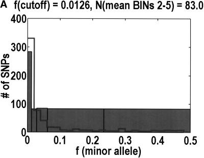
The main point of departure in our analyses of the NON/SYN ratio as a function of the minor allele frequency is that we partition the frequency axis into five histogram bins instead of three. One must be sensitive to the limitations imposed by having sampled only 44 diploid individuals in so many genes, as it means that the minor allele frequencies are essentially discretized in multiples of 1/(2*44) = 0.0114. It is critical that every histogram bin capture at least one of these discrete units. Specifically, we partitioned the frequency axis at 0.0000, 0.0126, 0.0280, 0.0614, 0.2346, and 0.5000. Bin 1 is meant to capture the singlets, that is, those SNPs that are observed in only one heterozygote. To accommodate the occasional sample failures, we set the upper bound to 0.0126 instead of 0.0114. The other four bins are designed to each capture an approximately equal number of coding SNPs, to equalize their statistical properties. We had the computer look at the actual distribution of allele frequencies above 0.0126, and then set the remaining partitions to make the number of coding SNPs per bin as uniform as possible. As so defined, bin 2 captures the doublets, whereas bin 3 captures the triplets, quadruplets, and quintuplets.
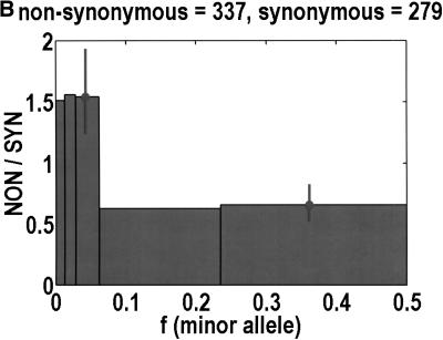
Figure 1 shows that, as a function of minor allele frequency, the NON/SYN ratio exhibits a threshold at a frequency of 0.0614, ∼6%. By this, we do not only mean that bins 3 and 5 are significantly different (P = 0.0032, Fisher's exact test). What is more interesting is that the differences between bins 1 to 3 are negligible. The NON/SYN ratio for singlets and other SNPs below 1% frequency—that regime traditionally associated with rare Mendelian diseases—is not very different from SNPs of up to 6%. Given so few bins, our frequency resolution is limited. It is likely that the transition is spread out over a finite range of frequencies. The size of this transition region is not particularly important. What matters is the existence of an inflection point in the frequency dependence, because this imposes a mathematical constraint on potential models for the data. How we partition the frequency axis affects the NON/SYN ratio for bin 2, but as long as we capture at least one discrete unit in bin 2, the threshold is robust.
Figure 1.
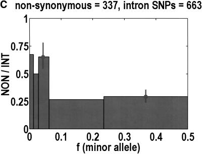
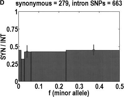
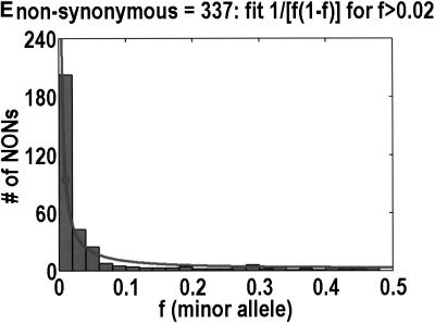
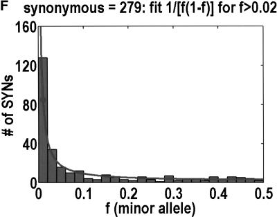
To analyze ratios for the number of SNPs that are deemed nonsynonymous (NON), synonymous (SYN), and intron (INT), we partition the frequency axes into 5 nonuniform bins with boundaries 0.0000, 0.0126, 0.0280, 0.0614, 0.2346, and 0.5000. There are 284 coding SNPs in bin 1, and there is a mean of 83.0 coding SNPs in each of the bins 2–5. These panels depict (A) the number of coding SNPs, with a solid line for the same data plotted on a uniform bin size of 0.02, (B) the NON/SYN ratio, (C) the NON/INT ratio, and (D) the SYN/INT ratio. Error bars indicate standard deviation, assuming the data are sampled from a binomial distribution. All of the uncertainty is in bins 2–5. Error bars for bin 1 are much smaller and not indicated. The generally lower quality of the intron data is responsible for the glitch in bin 2 of panels C and D. At top of each panel, we indicate the number of SNPs in the stated categories. Finally, we demonstrate the futility of trying to make sense of these data by more conventional methods. Using a uniform bin size of 0.02, we plot the number of (E) NON and (F) SYN polymorphisms, and compare them with the neutral theory expectation of 1/[f(1-f)]. Our curve fitting procedures ignore the first bin to avoid the singlets and sampling uncertainties. Extrapolation of the curve fit back to the first bin is indicated by a filled circle. Only if one squints hard enough at the fit deviations, might one notice a change in NON/SYN ratio.
One of the motivations for studying ratios like NON/SYN, instead of comparing NON or SYN directly to neutral theory expectations, is that the expected allele frequency distribution is confounded by the complexities of population history, which tend to affect the results at the low-frequency end, where we observe the threshold. Ratios offer a built-in control against much of this complexity, but to be safe, we wanted a second control, to ensure that nothing unusual is happening with the synonymous distribution itself, and that it behaves in an approximately neutral manner. Intron SNPs are the solution. As we show in Figure 1, comparisons against the intron data reveal that the threshold effect is due to changes in the nonsynonymous distribution, not changes in the synonymous distribution. This suggests that some kind of selection might be involved.
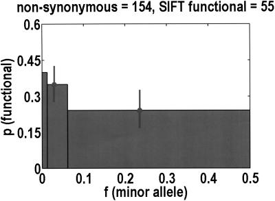
Considering how not every nonsynonymous SNP is functional, we were curious whether there was a second threshold effect for the probability that a nonsynonymous SNP is functional. We estimated this probability from the extent to which the polymorphic site is conserved across all available homologs in the public databases, using the program SIFT (Ng and Henikoff 2001). We do lose half of the data set by focusing on nonsynonymous SNPs, and another half of the data set because homologs are not always available. Therefore, to improve the statistics, we merge bins 2 + 3 and 4 + 5. Figure 2 demonstrates that there is likely to be a significant difference between bins 1 and 4 + 5 (P = 0.056, Fisher's exact test), but there are not enough data to compare bin 2 + 3 with its neighbors. Nevertheless, taking into account the probability that a nonsynonymous SNP is functional appears to amplify the threshold effect. If we accept the SIFT probabilities at face value, and normalize with respect to bin 2 + 3, the total number of functional nonsynonymous SNPs in bins 1, 2 + 3, and 4 + 5 is estimated to be 1.93, 1, and 0.44, respectively.
Figure 2.
The probability that a nonsynonymous SNP is functional is computed with the program SIFT, which considers the extent to which any polymorphic site is evolutionarily conserved across all good homologs in the public databases. Because only half of the nonsynonymous SNPs are SIFT analyzable, bin 1 is unchanged from Fig. 1, but bins 2 + 3 and 4 + 5 are merged together to improve statistics. Of these 154 analyzed SNPs, only 55 are predicted to be functional.
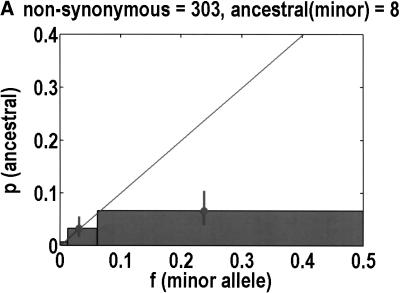
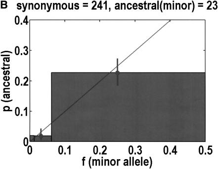
We can also test for departures from neutrality by determining the ancestral allele for each SNP, on the basis of orthologous chimpanzee and gorilla sequences. One chimpanzee and one gorilla sample was resequenced. Our experiments were successful in 544 of 616 coding SNPs. Of the rejects, 3 were eliminated because the primate alleles did not match either human allele, and 11 were ambiguous in that both human alleles were observed in the primates. PCR failures accounted for the remainder of the failures. The neutral theory expectation is that the probability of any allele being ancestral is equal to its frequency in the population (Watterson and Guess 1977). Again, we merged bins 2 + 3 and 4 + 5 to help improve statistics. Figure 3 emphasizes that synonymous SNPs behave as expected from neutrality, but nonsynonymous SNPs do not. In the latter case, it is bin 4 + 5 that exhibits the most significant deviation from neutrality (P = 0.0068, Fisher's exact test), but bin 2 + 3 does not have enough data to compare with expectations. In any case, it is not clear what we should expect, given how bin 4 + 5 deviates from neutrality. For example, if the correct background is a straight line of slope less than one, as determined by bin 4 + 5, one might say that there is a significant increase in bin 2 + 3.
Figure 3.
Ancestral alleles are determined by sequencing a chimpanzee and gorilla. We depict the probability that the minor allele is the ancestral allele. Bin 1 is unchanged from Fig. 1, but bins 2 + 3 and 4 + 5 are merged together to improve statistics. For each bin, we show the mean frequency as a filled circle. Data are divided into (A) nonsynonymous and (B) synonymous SNPs. Neutral theory predicts a straight line with a slope of 1, but this is observed only for synonymous SNPs.
Proposed Explanations
The original explanation that enrichment in low-frequency nonsynonymous SNPs is due to deleterious variants that have yet to be purified from the population must be re-examined in light of this 6% threshold. In the standard model, the likelihood that a simple recessive deleterious allele would reach 1% in frequency in a large population is thought to be astronomically small (Zwick et al. 2000). Deleterious alleles observed at above 1% have traditionally been attributed to balancing selection. For example, the high incidences of sickle cell anemia and other red blood cell disorders in tropical regions are attributed to the protection of the heterozygotes against severe malaria (Cooke and Hill 2001). What we observed is that the NON/SYN ratio for those SNPs below 1% in frequency is not all that different from those of up to 6%. This deserves an explanation.
Perhaps the simplest explanation is just to admit that the longstanding association of Mendelian diseases with variants of below 1% in frequency was always arbitrary, and that deleterious alleles and/or balancing selection are far more prevalent than commonly thought. If we had to choose, we would choose the former. Lack of change in NON/SYN below 6% implies a continuum of Mendelian diseases, presumably with reduced disease severity as allele frequencies increase. This follows from the equation for the equilibrium frequency in recessive deleterious alleles, f =  , where μ is the mutation rate and s is the selection coefficient. It is not clear to us how this would produce the observed behavior in the NON/SYN ratio as, for example, if we assume an exponential distribution, e-(s/so), for the selection coefficients, and adjust the parameters so that there are many alleles at a frequency of 2%–4%; then there would be almost none below 1%. Of course, we could always assume whatever distribution is required to get the desired result, but it does seem rather contrived. We decided instead to explore two more radical explanations, one based on the admixed nature of the HDP panel, and another based on adaptive selection. Notice that these explanations are not mutually exclusive.
The first explanation relies on the fact that some polymorphisms are found in all populations, and others are found only in specific populations. Suppose that synonymous SNPs have a frequency dependence S(f), and nonsynonymous SNPs have a frequency dependence [N1 + N2] · S(f), in which N1 is population independent and N2 is population specific. In a pure population, there would be no threshold effect. But, in a mixture of M populations, in which for simplicity we assume identical parameters for all populations, any population-specific SNP of frequency f in the source population would have an apparent frequency of f′ = f/M when averaged over the mixture. Hence, there would be two components to the NON/SYN ratio. For f′ > 0.5/M, this ratio would be N1, whereas for f′ ≤ 0.5/M, this ratio would be N1 + N2 · S(Mf′)/S(f′). One could explain the threshold effect simply by assuming appropriate values of M, N1, and N2.
We can estimate the appropriate parameters from our observed data. If we assume that M = 8, the apparent threshold frequency would be 0.0625. Given that the HDP panel is a 2:1:1 mixture of three major populations (European, African, Asian), one might argue that that is not a justifiable assumption, and that the observed 6% threshold frequency is, at worst, a few times smaller than it would have been in a pure population. But, given the method by which these samples were collected, we cannot rule out additional complexity in the underlying population structure. Moving on, if one assumes that f is not too close to zero, the standard model would predict that S(f) ∝ 1/f, which reduces S(Mf′)/S(f′) to a constant 1/M. Given that the observed NON/SYN ratios, above and below threshold, are 0.64 and 1.53, this implies that N2/N1 = M · (1.53/0.64 - 1) = 11. In other words, there are 11 population-specific SNPs for every population-independent one. In contrast, previous analyses of admittedly nonfunctional polymorphisms have consistently found that most human genetic variation is not population-specific (Barbujani et al. 1997). It would be fascinating if restricting the analyses to SNPs that are likely to be functional should turn this conclusion on its head.
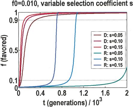
Should the first explanation be too disturbing, we can offer a second, on the basis of the temporal dynamics of how adaptive variants are fixed. Notice that by adaptive, we mean in the evolutionary sense, which has no implications for post-reproductive phenotypes. In fact, it has been argued that loss-of-function might be the preferred adaptive response in a rapidly changing environment (Olson 1999). Figure 4 illustrates the predicted increase in frequency of the favored allele, per generation, for either dominant or recessive modes of inheritance (Hartl 2000), and assuming large populations with weak selection. We used a range of selection coefficients taken from a survey of published experiments (Kingsolver et al. 2001), consisting of >2500 estimates in 62 species of vertebrates, invertebrates, and plants. These data are exponentially distributed with a 0.16 median. They are almost certainly biased against the smaller selection coefficients, which are difficult to measure. Nonetheless, they are the correct estimates, if the threshold is a leading edge effect due to favored alleles with the largest selection coefficients.
Figure 4.
Growth in the frequency of the favored allele per generation, with dominant (D) and recessive (R) modes of inheritance. Predicted behavior is given for a range of linear selection coefficients s. Allele frequency for time zero is fixed at f0 = 0.010. The recessive mode behavior is sensitive to f0, in that it affects when the rapid transition from 0.1 to 0.9 can occur. Regardless of settings, this transition is always fast, relative to the asymptotic behavior at one or the other end.
Regardless of the parameter settings or the mode of inheritance, transitions from frequencies of 0.1–0.9 are always fast, taking just a few dozen generations. In dominant mode, the favored allele quickly rises to 0.9 in frequency, and then it slows down, taking another 500 generations to reach its asymptote. Conversely, in recessive mode, the initial drift to 0.1 in frequency takes 500 generations or more, but afterward, the favored allele is quickly fixed. Precisely when this rapid transition from 0.1–0.9 occurs is sensitive to the initial frequency, which may be larger than one over the population size, as genetic variations can accumulate through mutation-selection balance (Orr and Betancourt 2001), buffered by protein chaperones (Rutherford and Lindquist 1998), and primed to respond to any changes in the environment. If we take a snapshot of the process before it has time to finish, relatively few SNPs would be found between 0.1 and 0.9. Without the ancestral data, one would only perceive an increase in SNPs of minor allele frequencies below 0.1. The beauty of this explanation is that a threshold of approximately the right frequency is predicted without assuming any contrived distributions.
An important point worth emphasizing is that we are envisioning a transient effect from a massive one-time change in the environment. In contrast, most theoretical models, including the more sophisticated Poisson random field (Bustamante et al. 2001), assume a steady state (equilibrium), in which new mutations are continuously created, then selected for/against, in a fixed environmental background. Furthermore, we make no assumptions about the mode of inheritance. There must be a distribution, but we do not know what it is. Therefore, even with our ancestral data, we cannot interpret a paucity of SNPs above 0.9 as evidence against adaptive selection, because if most of the adaptive variants are recessive, and the number of generations since time zero is about 500, most of these SNPs should be below 0.1 in frequency. These particular numbers are important, because we have in mind a very specific one-time event.
If we multiply 500 generations by a nominal human generation time of 20 yr, we get 10,000 yr. This neatly coincides with the end of the last ice age, the melting of the glaciers, and the development of agriculture—all of which happened 7,000∼17,000 yr ago. These events had a profound effect on the ways that we live, in the foods that we eat, the pathogens that we are exposed to, and ultimately, lead to human civilization (Diamond 2002). Of course, to establish that this was the causative event, we would need to do a negative control, say on an aboriginal population like the Yanomami from Brazil. Lacking this data, we can only speculate on how ironic it would be if, as we changed our own environment with these various activities, the changes were repaid through changes in the underlying genetic makeup of the human species itself.
DISCUSSION
One might wonder why such a simple effect had never been observed before. The answer is that surprisingly few people have been in any position to look for it. Despite the massive amounts of SNP (Sachidanandam et al. 2001) and microsatellite (Rosenberg et al. 2002) data that have been acquired, these data are not applicable to this phenomenon. Absent an explicit enrichment for nonsynonymous SNPs that are likely to be functional, the threshold would be buried in noise. Moreover, few data sets mea sure allele frequency to the necessary resolution in any population. In those few instances in which the SNP data met all the necessary conditions to observe the threshold the data were not plotted in such a way that the threshold could have been seen. As we show in Figure 1, it is nearly impossible to see the threshold from a simple frequency distribution for nonsynonymous and synonymous SNPs. Only when you look at the ratio of NON/SYN is the threshold obvious. Moreover, Cargill et al. (1999) set their first bin to 0%–5%, which precluded them from noticing that the NON/SYN ratio does not change from frequencies below 1% all the way up to 6%.
As for our more radical explanations, there is a major caveat on the applicability of the second explanation regarding adaptive selection to agriculture. We only sequenced 114 genes. This is a small subset of the 30,000–40,000 genes in the genome, and it is a biased subset at that, carefully selected for potential relevance to environmental diseases. Recall the assumptions that went into our model. We required the existence of a selection coefficient on the high end of what had been measured. Because most gene knockouts show no obvious phenotypes (Tautz 2000), large selection coefficients are likely to be rare, in which case the threshold might only be observable for the small fraction of human genes with the largest selection coefficients. This is nevertheless an important fraction, because these are the genes in which genetic variations will have major phenotypic consequences. Because we made no other assumptions about the nature of the functional polymorphism, the threshold is not necessarily limited to nonsynonymous SNPs. It might apply to intron SNPs too. For example, in another similar experiment, insertion-deletion polymorphisms identified in a special class of minimal introns appeared to be functional only for minor allele frequencies of below 6% (Yu et al. 2002).
Aside from being a potentially important clue to understanding the basis of human genetic variation, the threshold has a practical implication for the HapMap Project, which hopes to unravel the genetic basis of important complex diseases (Couzin 2002). The plan is to build haplotypes of high frequencies, certainly above 6%, under the assumption that susceptibilities for common diseases are due to a small number of ancient polymorphisms that occur at high frequencies in all populations (Lander 1996; Reich and Lander 2001). This assumption has been very harshly criticized (Terwilliger and Weiss 1998; Pritchard and Cox 2002; Weiss and Clark 2002; Wright et al. 2003). If the majority of the disease susceptibility SNPs lie under the threshold, there may be problems correlating haplotypes of frequency above 6% to disease susceptibility SNPs of frequency below 6%, as they could have arisen from very different population histories.
There will be no definitive answers until a larger number of genes are studied in a larger population sample with a better-defined history. Nevertheless, it is instructive how, by focusing the experiments on SNPs that are likely to be functional, and dividing out the complexities of population history, one can discover an interesting anomaly that stands as a challenge to the existing conceptual framework.
METHODS
PCR primers were placed on the introns. The objective was to acquire, along with the targeted exon, 100 bp of flanking intron sequence on each side. Short 1-Kb amplicons were chosen. Sequencing was performed by capillary electrophoresis and dyeterminator chemistry. We took the NHGRI/Coriell Human Diversity Panel (HDP) as a representative of all the major populations. For ancestral alleles, we used the human-specific primers to sequence chimpanzee and gorilla. Initial polymorphism detection was done by PolyPhred (Nickerson et al. 1997), and confirmed by visual inspection of the sequence traces. Many singlet SNPs, those observed in a single heterozygote, were validated by a reverse-strand read, especially in the coding region, in which 112 of 252 singlets were so validated versus 9 of 203 in the introns. Coupled with the fact that the intron data always lie at one or the other end of the reads, in which the data qualities are poor, we expect the overall results to be less accurate for intron SNPs. Although three of our genes had multiple hits to a database of recent segmental duplications (Bailey et al. 2002), only one of the SNPs identified in these genes exhibited a significant deviation from Hardy-Weinberg equilibrium. This one SNP was removed. All summarized SNPs had a minimum of 32 genotypes. For the SIFT analysis, we tried both the entire protein sequence and a 400-residue fragment centered at the SNP. Where there was a dispute, we favored the more intolerant prediction. Our data were submitted to dbSNP/GenBank under UWGC.
Acknowledgments
We thank Maynard Olson, Joe Felsenstein, and Pauline Ng for their help with the manuscript. This project was sponsored by the National Institute of Environmental Health Sciences (Grant no. 1 RO1 ES09909) and the National Human Genome Research Institute (Grant no. 1 P50 HG02351).
The publication costs of this article were defrayed in part by payment of page charges. This article must therefore be hereby marked “advertisement” in accordance with 18 USC section 1734 solely to indicate this fact.
Article and publication are at http://www.genome.org/cgi/doi/10.1101/gr.1324303.
References
- Bailey, J.A., Gu, Z., Clark, R.A., Reinert, K., Samonte, R.V., Schwartz, S., Adams, M.D., Myers, E.W., Li, P.W., and Eichler, E.E. 2002. Recent segmental duplications in the human genome. Science 297: 1003-1007. [DOI] [PubMed] [Google Scholar]
- Barbujani, G., Magagni, A., Minch, E., and Cavalli-Sforza, L.L. 1997. An apportionment of human DNA diversity. Proc. Natl. Acad. Sci. 94: 4516-4519. [DOI] [PMC free article] [PubMed] [Google Scholar]
- Bustamante, C.D., Wakeley, J., Sawyer, S., and Hartl, D.L. 2001. Directional selection and the site-frequency spectrum. Genetics 159: 1779-1788. [DOI] [PMC free article] [PubMed] [Google Scholar]
- Cargill, M., Altshuler, D., Ireland, J., Sklar, P., Ardlie, K., Patil, N., Shaw, N., Lane, C.R., Lim, E.P., Kalyanaraman, N., et al. 1999. Characterization of single-nucleotide polymorphisms in coding regions of human genes. Nat. Genet. 22: 231-238. [DOI] [PubMed] [Google Scholar]
- Collins, F.S., Brooks, L.D., and Chakravarti, A. 1998. A DNA polymorphism discovery resource for research on human genetic variation. Genome Res. 8: 1229-1231. [DOI] [PubMed] [Google Scholar]
- Cook, G.S. and Hill, A.V. 2001. Genetics of susceptibility to human infectious disease. Nat. Rev. Genet. 2: 967-977. [DOI] [PubMed] [Google Scholar]
- Couzin, J. 2002. New mapping project splits the community. Science 296: 1391-1393. [DOI] [PubMed] [Google Scholar]
- Diamond, J. 2002. Evolution, consequences and future of plant and animal domestication. Nature 418: 700-707. [DOI] [PubMed] [Google Scholar]
- Fay, J.C., Wyckoff, G.J., and Wu, C.I. 2001. Positive and negative selection on the human genome. Genetics 158: 1227-1234. [DOI] [PMC free article] [PubMed] [Google Scholar]
- Halushka, M.K., Fan, J.B., Bentley, K., Hsie, L., Shen, N., Weder, A., Cooper, R., Lipshutz, R., and Chakravarti, A. 1999. Patterns of single-nucleotide polymorphisms in candidate genes for blood-pressure homeostasis. Nat. Genet. 22: 239-247. [DOI] [PubMed] [Google Scholar]
- Harpending, H. and Rogers, A. 2000. Genetic perspectives on human origins and differentiation. Annu. Rev. Genomics Hum. Genet. 1: 361-385. [DOI] [PubMed] [Google Scholar]
- Hartl, D.L. 2000. A primer of population genetics. 3d ed. Sinauer Associates, Sunderland, MA.
- Kimura, M. 1983. The neutral theory of molecular evolution. Cambridge University Press, Cambridge, UK.
- Kingsolver, J.G., Hoekstra, H.E., Hoekstra, J.M., Berrigan, D., Vignieri, S.N., Hill, C.E., Hoang, A., Gibert, P., and Beerli, P. 2001. The strength of phenotypic selection in natural populations. Am. Nat. 157: 245-261. [DOI] [PubMed] [Google Scholar]
- Lander, E.S. 1996. The new genomics: Global views of biology. Science 274: 536-539. [DOI] [PubMed] [Google Scholar]
- Ng, P.C. and Henikoff, S. 2001. Predicting deleterious amino acid substitutions. Genome Res. 11: 863-874. [DOI] [PMC free article] [PubMed] [Google Scholar]
- Nickerson, D.A., Tobe, V.O., and Taylor, S.L. 1997. PolyPhred: Automating the detection and genotyping of single nucleotide substitutions using fluorescence-based resequencing. Nucleic Acids Res. 25: 2745-2751. [DOI] [PMC free article] [PubMed] [Google Scholar]
- Olson, M.V. 1999. When less is more: Gene loss as an engine of evolutionary change. Am. J. Hum. Genet. 64: 18-23. [DOI] [PMC free article] [PubMed] [Google Scholar]
- Orr, H.A. and Betancourt, A.J. 2001. Haldane's sieve and adaptation from the standing genetic variation. Genetics 157: 875-884. [DOI] [PMC free article] [PubMed] [Google Scholar]
- Pritchard, J.K. and Cox, N.J. 2002. The allelic architecture of human disease genes: Common disease—common variant... or not? Hum. Mol. Genet. 11: 2417-2423. [DOI] [PubMed] [Google Scholar]
- Przeworski, M., Hudson, R.R., and Di Rienzo, A. 2000. Adjusting the focus on human variation. Trends Genet. 16: 296-302. [DOI] [PubMed] [Google Scholar]
- Reich, D.E. and Lander, E.S. 2001. On the allelic spectrum of human disease. Trends Genet. 17: 502-510. [DOI] [PubMed] [Google Scholar]
- Rosenberg, N.A., Pritchard, J.K., Weber, J.L., Cann, H.M., Kidd, K.K., Zhivotovsky, L.A., and Feldman, M.W. 2002. Genetic structure of human populations. Science 298: 2381-2385. [DOI] [PubMed] [Google Scholar]
- Rutherford, S.L. and Lindquist, S. 1998. Hsp90 as a capacitor for morphological evolution. Nature 396: 336-342. [DOI] [PubMed] [Google Scholar]
- Sachidanandam, R., Weissman, D., Schmidt, S.C., Kakol, J.M., Stein, L.D., Marth, G., Sherry, S., Mullikin, J.C., Mortimore, B.J., Willey, D.L., et al. 2001. A map of human genome sequence variation containing 1.42 million single nucleotide polymorphisms. Nature 409: 928-933. [DOI] [PubMed] [Google Scholar]
- Stephens, J.C., Schneider, J.A., Tanguay, D.A., Choi, J., Acharya, T., Stanley, S.E., Jiang, R., Messer, C.J., Chew, A., Han, J.H., et al. 2001. Haplotype variation and linkage disequilibrium in 313 human genes. Science 293: 489-493. [DOI] [PubMed] [Google Scholar]
- Tautz, D. 2000. A genetic uncertainty problem. Trends Genet. 16: 475-477. [DOI] [PubMed] [Google Scholar]
- Terwilliger, J.D. and Weiss, K.M. 1998. Linkage disequilibrium mapping of complex disease: Fantasy or reality? Curr. Opin. Biotechnol. 9: 578-594. [DOI] [PubMed] [Google Scholar]
- Waterston, R.H., Lindblad-Toh, K., Birney, E., Rogers, J., Abril, J.F., Agarwal, P., Agarwala, R., Ainscough, R., Alexandersson, M., An, P., et al. 2002. Initial sequencing and comparative analysis of the mouse genome. Nature 420: 520-562. [DOI] [PubMed] [Google Scholar]
- Watterson, G.A. and Guess, H.A. 1977. Is the most frequent allele the oldest? Theor. Popul. Biol. 11: 141-160. [DOI] [PubMed] [Google Scholar]
- Weiss, K.M. and Clark, A.G. 2002. Linkage disequilibrium and the mapping of complex human traits. Trends Genet. 18: 19-24. [DOI] [PubMed] [Google Scholar]
- Wright, A., Charlesworth, B., Rudan, I., Carothers, A., and Campbell, H. 2003. A polygenic basis for late-onset disease. Trends Genet. 19: 97-106. [DOI] [PubMed] [Google Scholar]
- Yu, J., Yang, Z., Kibukawa, M., Paddock, M., Passey, D.A., and Wong, G.K.S. 2002. Minimal introns are not “junk”. Genome Res. 12: 1185-1189. [DOI] [PMC free article] [PubMed] [Google Scholar]
- Zwick, M.E., Cutler, D.J., and Chakravarti, A. 2000. Patterns of genetic variation in Mendelian and complex traits. Annu. Rev. Genomics Hum. Genet. 1: 387-407. [DOI] [PubMed] [Google Scholar]
WEB SITE REFERENCES
- http://www.genome.washington.edu/projects/egpsnps; University of Washington Genome Center Repository of Candidate-Gene Polymorphisms for Environmental Genome Project (EGP).


