A finite rate of innovation algorithm for fast and accurate spike detection from two-photon calcium imaging

Abstract

Objective

Inferring the times of sequences of action potentials (APs) (spike trains) from neurophysiological data is a key problem in computational neuroscience. The detection of APs from two-photon imaging of calcium signals offers certain advantages over traditional electrophysiological approaches, as up to thousands of spatially and immunohistochemically defined neurons can be recorded simultaneously. However, due to noise, dye buffering and the limited sampling rates in common microscopy configurations, accurate detection of APs from calcium time series has proved to be a difficult problem.

Approach

Here we introduce a novel approach to the problem making use of finite rate of innovation (FRI) theory (Vetterli et al 2002 IEEE Trans. Signal Process. 50 1417–28). For calcium transients well fit by a single exponential, the problem is reduced to reconstructing a stream of decaying exponentials. Signals made of a combination of exponentially decaying functions with different onset times are a subclass of FRI signals, for which much theory has recently been developed by the signal processing community.

Main results

We demonstrate for the first time the use of FRI theory to retrieve the timing of APs from calcium transient time series. The final algorithm is fast, non-iterative and parallelizable. Spike inference can be performed in real-time for a population of neurons and does not require any training phase or learning to initialize parameters.

Significance

The algorithm has been tested with both real data (obtained by simultaneous electrophysiology and multiphoton imaging of calcium signals in cerebellar Purkinje cell dendrites), and surrogate data, and outperforms several recently proposed methods for spike train inference from calcium imaging data.

1. Introduction

Understanding how information processing occurs in neural circuits is one of the principal problems of systems neuroscience. Information is encoded in the firing of action potentials (APs, or spikes) by individual neurons, and information processing involves the coordination of AP firing by large populations of neurons organized into neural circuits. To understand neural information processing, we thus must monitor the activity of neural circuits at a spatial resolution sufficient to resolve many individual neurons, and a temporal resolution sufficient to resolve individual APs on individual experimental trials. Of the currently available techniques for conducting neurophysiological experiments, only multiphoton calcium imaging (Denk et al 1990, 1994, Svoboda et al 1999, Stosiek et al 2003) and multielectrode array electrophysiology (Csicsvari et al 2003, Blanche et al 2005, Du et al 2009) offer this capability. Of these, only multiphoton calcium imaging currently allows precise three-dimensional localization of each individual monitored neuron within the region of tissue studied, in the intact brain.

In order to monitor cellular activity, neurons must be labelled with a fluorescent indicator, and a number of approaches have been used to do this. Single cells can be labelled by filling the cell with dye during a whole-cell or intracellular recording (Kitamura et al 2008, Helmchen et al 1999). Alternatively, populations of neurons can be simultaneously labelled with acetoxy-methyl (AM) ester calcium dyes (Stosiek et al 2003), allowing simultaneous monitoring of AP induced calcium signals in a plane (Ohki et al 2005) or volume (Göbel and Helmchen 2007) of tissue. To investigate information processing in neural circuits, it is necessary to relate these calcium signals to the properties of the spike trains fired by the neurons, ideally by detecting the times of occurrence of spikes with single AP resolution. A number of methods have previously been used to detect spike trains from calcium imaging data, including thresholding the first derivative of the calcium signal (Smetters et al 1999), and the application of template-matching algorithms based on either fixed exponential (Kerr et al 2005, 2007, Greenberg et al 2008) or data-derived (Schultz et al 2009, Ozden et al 2008) templates. Machine learning techniques (Sasaki et al 2008) and probabilistic methods based on sequential Monte Carlo framework (Vogelstein et al 2009) or fast deconvolution (Vogelstein et al 2010) have also been proposed.

Some broadly used methods such as template matching or derivative-thresholding have the disadvantage that they do not deal well with multiple events occurring within a time period comparable to the sampling interval. Unfortunately, given that laser-scanning two-photon imaging systems are largely limited to scan rates of 8–30 Hz when frame-scanning with sufficient spatial resolution to capture many neurons, and that neurons in many brain areas have a propensity to fire spikes in bursts, this is a relatively common occurrence in neurophysiological calcium signals. Bursts of spikes have been found to convey information with high reliability in some sensory systems (Reinagel et al 1999, Gabbiani et al 1996), and have been suggested to carry distinct sensory signals (Wang et al 2007). It is thus desirable to develop calcium transient detection algorithms that accurately detect multiple spike calcium events. As there is a trade-off between the area of tissue imaged and signal to noise ratio (SNR) (zooming in on a region of tissue allows the collection of more photons per neuron, thus offering better SNR, but limits the number of neurons that can be studied) and similarly between sampling rate and the area of tissue that can be imaged, it is desirable to improve algorithms for the detection of APs from calcium fluorescence time series.

In this paper we present a novel approach that extends modern sampling theory based on finite rate of innovation (FRI) theory. In the absence of noise, the FRI algorithm perfectly retrieves the locations of APs using a variation of a fast non-iterative algebraic method called annihilating filter (a.k.a. Prony’s method). This method reconstructs complex exponentials in noise from a set of samples. We have combined this with a novel double consistency sliding window technique that improves performances in noisy scenarios. To reconstruct the time series we construct a Toeplitz matrix from the samples. The key characteristic of this matrix is that, in the noiseless case, it is rank deficient, and its rank is always equal to the number of APs in the observation window. We run the algorithm twice, firstly with a large time window to estimate the number of spikes by singular value decomposition (SVD), and secondly, with a time window containing only a small number of spikes. In both cases, for each position of the sliding window, the algorithm outputs the locations of the K spikes assumed within the window. When the estimate of K is correct, the retrieved locations are stable among different sliding windows, and when incorrect, unstable. We construct a joint histogram of the retrieved locations with the two different window sizes. The final spike time estimates are obtained from histogram peaks, corresponding to consistent positions among different windows.

The proposed algorithm is robust in high noise scenarios, and fast enough to allow real-time spike train inference for tens of neurons. We show that for surrogate data with a temporal resolution of 27 Hz and a SNR of 10 dB the algorithm presents a spike detection rate above 95% with a false-positive rate below 0.02 Hz. Moreover, this algorithm is able to retrieve the spike locations with a precision higher than the temporal resolution of the acquired data.

2. Methods

2.1. Experimental methods

The data used in this study, and the experimental methods used to collect them, have been previously described (Schultz et al 2009). Briefly, Sprague-Dawley rats (P18–P29) were anaesthetized with urethane (1.2 g kg⁻¹) or with ketamine (50 mg kg⁻¹) / xylazine (5 mg kg⁻¹). A craniotomy was made over area Crus IIa of the cerebellum, filled with 1.5–2% agarose in Ringer’s solution, and a coverslip clamped above the agarose to suppress brain movement, while leaving a window open for microelectrode access. A micropipette was inserted to a depth of around 100–200 μm below the pia mater, and AM-ester calcium dye (Oregon Green BAPTA-1 AM) pressure-ejected. Imaging was performed from 30 min following dye ejection, using a two-photon laser scanning microscope (Prairie Technologies). A pulsed Titanium:Sapphire laser was used for excitation, operating at 810 nm (MaiTai, SpectraPhysics) with <100 fs pulse width and 80 MHz repetition rate, and focused using a 40×, 0.8 Numerical Aperture objective lens (Olympus).

Image frames were acquired using ScanImage software (Pologruto et al 2003) for MATLAB (MathWorks). Raster lines making up each frame were of 2 or 2.3 ms duration, resulting in frame rates of 7–16 Hz. For each region imaged, a high resolution reference image was first acquired (512 × 512 pixels, average of five frames), followed by movies at 256 × 64 or 256 × 32 pixel resolution. Fluorescence time series for each neuron were obtained by defining regions of interest (ROIs) using a combination of human operator and spatial independent component analysis (Schultz et al 2009, Reidl et al 2007), and for each time bin, averaging the values of each pixel within the ROI.

To validate our event detection algorithms, we simultaneously performed targeted extracellular recordings from imaged neurons. Patch micropipettes (~4 MΩ) were filled with artificial cerebrospinal fluid (ACSF), together with Alexa 594 to aid visualization of the pipette. The pipette was navigated until the tip was adjacent to a Purkinje cell soma or dendrites and CS could be observed with high SNR. We emphasize that we are using two-photon targeted (visualized) juxtacellular recording, using a patch-pipette filled with dye. Using this technique, we can observe that the pipette is attached to a cell in which fluorescence changes are observed for each AP, meaning that there is no ambiguity concerning which cell is being recorded from. Electrophysiological and imaging data were then simultaneously acquired from the same neuron (figure 1).

Figure 1.

Simultaneous multiphoton calcium imaging with electrophysiology. (a) Maximum intensity projection showing juxtacellular recording from a Purkinje cell dendrite. The tissue was loaded with Oregon Green BAPTA-1 AM calcium indicator dye (green), and the pipette filled with Alex 594 (red) to aid visualization during targeted recording. (b) Imaged location, corresponding to grey horizontal line in (a). (c) Mask showing region of interest for the recorded Purkinje cell. (d) Simultaneous acquisition of fluorescence time series (shown unfiltered) and dendritically recorded complex spikes (CS), showing CS-driven calcium transients.

2.2. Mathematical model

At time t we consider the fluorescence measurement for a given ROI to be proportional to the calcium concentration plus additive Gaussian noise (Vogelstein et al 2009):

$$F_t=\alpha {\left[{\mathrm{Ca}}^{2+}\right]}_t+\beta +{∊}_t,$$ (2.1)

where [Ca²⁺]_t is the intracellular calcium concentration at time t, constant β represents the baseline calcium concentration of a particular cell and ∊_t the noise at time t. The noise is independently and identically distributed according to a normal distribution with zero mean and σ² variance.

The signal that we will consider is the normalized fluorescence

$$\Delta F_t∕F_0=\frac{F_t-F_0}{F_0},$$ (2.2)

abbreviated as ΔF/F. F₀ is the average background pre-stimulus fluorescence.

To model mathematically the calcium dynamics [Ca²⁺]_t, some assumptions have to be made (Vogelstein et al 2009). We assume that when a neuron is activated, the calcium concentration jumps instantaneously, and each jump has the same amplitude A. The concentration then decays exponentially with time constant τ, to a baseline concentration. The one-dimensional fluorescence signal can therefore be characterized by convolving the spike train with a decaying exponential and adding noise:

$$\begin{array}{cc}\hfill \Delta F∕F=& A\sum _k{\mathrm{e}}^{-(t-t_k)∕\tau }u(t-t_k)+{∊}_t\hfill \\ \hfill =& A\sum _k\delta (t-t_k)\ast {\mathrm{e}}^{-t∕\tau }u\left(t\right)+{∊}_t,\hfill \end{array}$$ (2.3)

where the index k represents different spikes, the different t_k their occurrence times and u(t) the unit step function. Hence, the goal of the spike detection algorithm is to obtain the values t_k.

2.3. Spike detection

Our spike detection algorithm is based on connecting the calcium transient estimation problem to the theory of FRI signals. We therefore first provide an overview of this theory and then present our spike detection method.

2.3.1. Overview of FRI theory

FRI theory applies to specific classes of signals which are completely specified by a finite number of free parameters. The goal of FRI algorithms is to reconstruct a signal that best fit the model given the available measurements. This is achieved by building specific matrices whose singular values and singular vectors provide the information necessary to retrieve the free parameters of the signals. Specifically, the canonical expression of a signal with FRI is given by:

$$x\left(t\right)=\sum _{k\in \mathbb{Z}}{a}_{k}g(t-t_k).$$ (2.4)

If the function g(t) is known, the signal x(t) is completely determined by the coefficients a_k and the shifts t_k, these are the free parameters. Introducing a counting function C_x(t_a, t_b) that counts the free parameters or degrees of freedom of x(t) over the time interval [t_a, t_b], the rate of innovation is defined as (Vetterli et al 2002)

$$\rho =\underset{\tau \to \infty }{\lim }\frac{1}{\tau }{C}_x\left(-\frac{\tau }{2},\frac{\tau }{2}\right).$$ (2.5)

We can then define FRI signals as those with a finite ρ. A typical example of such signals is a stream of K Diracs, $x\left(t\right)={\sum }_{k=1}^K{a}_k\delta (t-t_k)$. This signal is not-bandlimited, but we only need to know the K pair of coefficients (a_k, t_k) to perfectly reconstruct it. Classical sampling theory does not allow sampling and perfect reconstruction of this type of signal. However, recent work in FRI theory has shown that this is possible (Vetterli et al 2002). In the sequel we show how it is possible to acquire the signal $x\left(t\right)={\sum }_{k=1}^K{a}_k\delta (t-t_k)$ and perfectly reconstruct it from a finite set of samples.

Acquisition devices are usually modelled as a filtering stage followed by a sampling stage as illustrated in figure 2. Filtering signal x(t) with h(t) = ψ(−t/T) and retrieving samples at instants of time t = nT is equivalent to computing the inner product between x(t) and ψ(t/T – n). Specifically, the filtered signal is given by

$$\begin{array}{cc}\hfill y\left(t\right)=& x\left(t\right)\ast h\left(t\right)\hfill \\ \hfill =& {\int }_{-\infty }^{+\infty }x\left(\tau \right)h(t-\tau )\mathrm{d}\tau \hfill \\ \hfill =& {\int }_{-\infty }^{+\infty }x\left(\tau \right)\psi \left(-\frac{t-\tau }{T}\right)\mathrm{d}\tau .\hfill \end{array}$$ (2.6)

Figure 2.

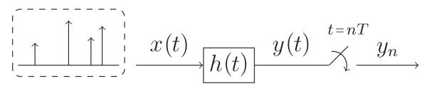
Filtering and sampling.

Moreover, sampling y(t) at regular intervals of time t = nT leads to

$$\begin{array}{cc}\hfill y_n=& y\left(t\right){\mid }_{t=\mathit{nT}}\hfill \\ \hfill =& {\int }_{-\infty }^{+\infty }x\left(\tau \right)\psi \left(\frac{\tau }{T}-n\right)\mathrm{d}\tau \hfill \\ \hfill =& \langle x\left(t\right),\psi -\left(\frac{t}{T}-n\right)\rangle \hfill \end{array}$$ (2.7)

Hence, samples y_n correspond to the projection of x(t) onto the set of functions ${\left\{\psi \right(t∕T-n\left)\right\}}_{n\in \mathbb{Z}}$.

The function ψ(t) is called sampling kernel and has to satisfy specific properties to be able to perfectly reconstruct the signal x(t). Exponential reproducing kernels satisfy the required conditions (Dragotti et al 2007). This is a family of kernels that together with its shifted versions can reproduce exponentials of the form e^α_mt:

$$\sum _{n\in \mathbb{Z}}{d}_{m,n}\psi (t-n)={\mathrm{e}}^{{\alpha }_{m}t},$$ (2.8)

where m = 0, 1, … , P. This expression is satisfied for a proper choice of coefficients d_m,n. The computation of these coefficients is detailed in appendix A.1. The parameters α_m can be chosen arbitrarily. However we require α_m = α₀ + m_λ in order to be able to use the annihilating filter method described later on. Moreover, we choose them to be ${\alpha }_m=j\frac{\pi }{P}(m-\frac{P}{2})$. They are selected to be purely imaginary because they are more robust against noise and in complex conjugate pairs in order to have a real valued kernel ψ(t). E-splines are a type of functions that are able to reproduce exponentials and have the advantage of being of compact support (Urigüen et al 2011). An E-spline of order P can reproduce P + 1 different exponentials as in (2.8). Figure 3 shows an example with P = 1. This E-spline is able to reproduce two different exponentials.

Figure 3.

First order E-spline that reproduces two different exponential functions. (a) First order E-spline. (b) Reproduction of e⁻². (c) Reproduction of e^+t/2.

Given the samples y_n, we now want to retrieve the degrees of freedom ${\left\{\right(a_k,t_k\left)\right\}}_{k=1}^K$. If we combine these samples with coefficients d_m,n, we obtain

$$\begin{array}{cc}\hfill \sum _n{d}_{m,n}{y}_n& =\sum _n{d}_{m,n}\langle x\left(t\right),\psi (t-n)\rangle \hfill \\ \hfill & =\langle x\left(t\right),\underset{={\mathrm{e}}^{{\alpha }_{m}t}}{\underbrace{\sum _n{d}_{m,n}\psi (t-n)}}\rangle \hfill \\ \hfill & ={\int }_{-\infty }^{+\infty }x\left(t\right){\mathrm{e}}^{{\alpha }_{m}t}\mathrm{d}t=s_m,\hfill \end{array}$$ (2.9)

where m = 0, 1, … , P. The new samples s_m are the exponential moments of the signal x(t). In the particular case where the input signal is a stream of Diracs, and α_m can be written as α_m = α₀ + mλ, the exponential moments can be expressed as a sum of exponentials (see appendix A.2):

$$s_m=\sum _{k=1}^K{b}_k{u}_k^m,$$ (2.10)

where b_k = a_k e^α₀t_k and u_k = e^λt_k. We are now faced with the problem of having to retrieve b_k and u_k from the sequence s_m. The problem is linear in the parameters b_k, but it is nonlinear in the parameters u_k. Therefore the difficulty is in finding the nonlinear terms. We solve the problem by applying the annihilating filter method. The annihilating filter is a filter of length K + 1 with zeros at locations ${\left\{u_k\right\}}_{k=1}^K$. The z transform of the impulse response of the filter is thus

$$H\left(z\right)=\sum _{m=0}^K{h}_m{z}^{-m}=\prod _{k=1}^K(1-u_k{z}^{-1}).$$ (2.11)

This method is based on the observation that if we filter the sequence s_m with a filter with zeros at u_k the output is zero. To convince ourselves of this fact let us assume that we have a sequence with only one exponential: $s_m=u_1^m$. The corresponding annihilating filter is 1 – u₁ z⁻¹. This filter computes finite differences weighted by u₁. The output of the filter is thus s_m – u₁s_m–1. The sequence s_m is cancelled out as the weight u₁ is exactly the rate of growth of the sequence. If we have more than one exponential we can annihilate the signal by cascading unitary filters where each of them cancels out one exponential. Figure 4 illustrates this concept. The z transform of filters connected in series is the product of their transfer functions. Thus the transfer function of the annihilating filter is

$$H\left(z\right)=\sum _{m=0}^K{h}_m{z}^{-m}=\prod _{k=1}^K(1-u_k{z}^{-1})$$ (2.12)

and we have that

$$\begin{array}{cc}\hfill h_m\ast s_m=& \sum _{i=1}^K{h}_i{s}_{m-i}\hfill \\ \hfill =& \sum _{i=0}^K{h}_i\sum _{k=1}^K{b}_k{u}_k^{m-i}\hfill \\ \hfill =& \sum _{k=1}^K{b}_k{u}_k^m\underset{=H\left(u_k\right)}{\underbrace{\sum _{i=0}^K{h}_i{u}_k^{-i}}}=0,\hfill \end{array}$$ (2.13)

since $H\left(z\right){\mid }_{z=u_k}={\sum }_{m=0}^K{h}_m{u}_k^{-m}=0$. If 2K + 1 samples of s_m are available, the convolution h_m * s_m can be expressed in matrix form as Sh = 0:

$$\left(\begin{array}{ccc}\hfill s_K\hfill & \hfill \cdots \hfill & \hfill s_0\hfill \\ \hfill ⋮\hfill & \hfill \ddots \hfill & \hfill ⋮\hfill \\ \hfill s_{2K}\hfill & \hfill \cdots \hfill & \hfill s_K\hfill \end{array}\right)\left(\begin{array}{c}\hfill h_0\hfill \\ \hfill ⋮\hfill \\ \hfill h_K\hfill \end{array}\right)=\left(\begin{array}{c}\hfill 0\hfill \\ \hfill ⋮\hfill \\ \hfill 0\hfill \end{array}\right).$$ (2.14)

The matrix S is rank deficient with rank K; the system is therefore overdetermined and the solution is not unique. If we impose h₀ = 1, the system has a unique solution. Once h has been found, the locations t_k are directly determined from the roots of the polynomial H(z) as u = e^λt_k, where λ is the parameter of the coefficients α_m = α₀ + mλ. From (2.14) and imposing h₀ = 1, it can be seen that we need at least 2K samples s_m. This imposes a lower limit to the order P of the E-spline as we compute the measurements s_m for m = 0, 1, … , P, where P is its order.

Figure 4.

The annihilating filter is a cascaded interconnection of unitary filters with zeros at u_k. Any signal formed by a linear combination of the exponential sequences $u_k^n$ is filtered out.

Retrieval of the parameters of a sum of exponentials in noise in the form given in (2.10) is a recurrent problem in spectral estimation. We refer the reader to Stoica and Moses (2005) for further details.

The previous theory has been presented for continuous-time signals and an analogue sampling kernel. However it can easily be extended to discrete-time signals. We can assume that the independent variable t of the input signal x(t) is discrete. For a given temporal resolution T_res, we define discrete time values as t = nT_res, where $n\in \mathbb{Z}$. The filter is then replaced by a discretized version of ψ(t) and the convolution is computed as a summation instead of an integral. Moreover, if we set the sampling period at the output of the filter to be the temporal resolution, that is T = T_res, the sampling stage after the filter can be omitted, as the filter’s output y(t) is a discrete sequence that directly corresponds to samples y_n. The T = T_res condition also applies to the scaling factor of the kernel which becomes ψ(t/T_res).

2.3.2. Data processing

Based on the above framework, we now develop a method for spike detection in calcium transient signals. Recall that the input signal can be expressed as a stream of decaying exponentials. Moreover, we assume that there is a finite number K of spikes within the observation period. Therefore the noiseless calcium concentration variation, denoted c(t), can be expressed as

$$\begin{array}{cc}\hfill c\left(t\right)=& A\sum _{k=1}^K{\mathrm{e}}^{\alpha (t-t_k)}u(t-t_k)\hfill \\ \hfill =& \underset{x\left(t\right)}{\underbrace{\sum _{k=1}^K\delta (t-t_k)}}\ast \underset{{\rho }_{\alpha }\left(t\right)}{\underbrace{A{\mathrm{e}}^{-\alpha t}u\left(t\right)}}\hfill \\ \hfill =& x\left(t\right)\ast {\rho }_{\alpha }\left(t\right).\hfill \end{array}$$ (2.15)

Here the variable t is discrete. The detection process requires filtering the measured signal. The filter has an impulse response h(t) = φ(—t) where φ(t) is able to reproduce exponentials as in (2.8), specifically

$$\sum _{n\in \mathbb{Z}}{c}_{m,n}\phi (t-n)={\mathrm{e}}^{{\alpha }_{m}t}.$$ (2.16)

The signal c(t) is filtered with h(t) = φ(–t). The output of the filter h(t) are the samples y_n that correspond to the inner product between c(t) and shifted versions of the kernel: y_n = ⟨c(t), φ(t – n)⟩. Samples y_n can also be expressed as y_n = ⟨x(t), ρ_α(–t) * φ(t – n)⟩ (see appendix A.3). One of the key points of the previously described FRI framework is that the filtered and sampled stream of Diracs is combined with the d_m,n coefficients from (2.8) to obtain the sum of exponentials given in (2.10). It will become clearer in what follows, that despite the fluorescence signal being composed of a stream of decaying exponentials, this first filtering stage with the exponential reproducing function φ(t) will allow us to turn the problem into retrieving the locations of a stream of Diracs.

The next step of the algorithm is to compute finite weighted differences of samples y_n in order to obtain new samples z_n. This is a second filtering stage with a filter with transfer function G(z) = 1 – e^−αT z⁻¹. These steps are illustrated in figure 5. Filtering signal c(t) with φ(–t) and computing samples z_n = y_n – y_n−1 e^−αT is analogous to filtering the stream of Diracs x(t) with a different kernel ψ(t) (see appendix A.4). At this stage, the problem has been turned into a sampling process of a stream of Diracs. This new kernel, ψ(t), is still able to reproduce exponentials (Unser and Blu 2005). That is, there exists coefficients d_m,n such that ∑_n d_m,n ψ(t – n) = e^α_mt.

Figure 5.

Filtering process of the measured signal.

The problem of estimating the calcium transients and the problem of reconstructing an FRI signal are now equivalent. In fact, we now have a set of samples z_n = ⟨x(t), ψ(t – n)⟩ which are equivalent to those that we would obtain if we were sampling the stream of Diracs x(t) with the exponential reproducing kernel ψ(t). We can therefore apply FRI techniques to retrieve the location of the Diracs and, as highlighted in (2.15), those correspond exactly to the activation times of the APs. We summarize this inference method in algorithm 1.

Algorithm 1.

FRI spike train inference (noiseless scenario)

Input: c(t): calcium concentration, K: number of spikes

Output: ${\left\{t_k\right\}}_{k=1}^K$: spike locations

1: Filter with exponential reproducing kernel: yn = ⟨c(t), φ(t – n)⟩

2: Compute weighted finite differences: zn = yn – yn–1 e−αT

3: Obtain new measurements: sm = ∑n dm,n zn

4: Compute the annihilating filter: hm * sm = 0

5: Retrieve locations from roots of the annihilating filter: $H\left(z\right)={\sum }_{m=0}^K{h}_m{z}^{-m}={\prod }_{k=1}^K(1-u_k{z}^{-1})$, where uk = eλtk

2.3.3. Spike inference in practice

Real data presents two main issues. Firstly, in the presence of noise, the matrix S from (2.14) is not rank deficient. And secondly, the number of spikes (K) within a time interval is unknown.

In the noiseless case, the matrix S has rank K. The SVD of this matrix has therefore only K non-zero singular values. When noise is added to the input signal, the matrix S becomes full rank and if we do not have prior knowledge of K, estimating its value becomes part of the problem. In a low noise scenario and when K is not zero, K can be estimated from the singular values of S. In this case, the contribution of the signal in the singular value of S is more important than the contribution of the noise, and a clear separation can be established to estimate the number of singular values that are due to the signal.

Another effect of the noise is that equation (2.14) is not satisfied exactly. We have followed two different approaches to overcome this situation. The first approach (Blu et al 2008) starts with denoising the matrix S with an iterated algorithm (Cadzow 1988). The matrix S is Toeplitz by construction, but is not rank deficient due to the presence of noise. The iterated algorithm makes the matrix S be of rank K (using the previously estimated value of K) setting to zero the smallest singular values. This new matrix S′ has rank K but is not Toeplitz anymore. A new matrix is built averaging the diagonal elements of matrix S′. These two steps are repeated until some stop condition is reached. The next step is to solve equation (2.14). This is done computing the total least squares solution that minimizes ∥Sh∥² subject to ∥h∥² = 1 The second approach is based on the matrix pencil method (Hua and Sarkar 1990) which is in essence based on the same principle that is used in the ESPRIT algorithm (Paulraj et al 1985) for the estimation of directions of arrival of signals in arrays of antennas. This approach has already been successfully used in the FRI framework (Maravić and Vetterli 2005). This method is based on the particular structure of the matrix S, which is Toeplitz and each element is given by a sum of exponentials as shown in (2.10). Let S₀ be the matrix constructed from S by dropping the last row and S₁ the matrix constructed from S by dropping the first row. It can be shown that in the matrix pencil S₀ – μS₁ the parameters ${\left\{u_k\right\}}_{k=1}^K$ are rank reducing numbers, that is, the matrix S – μS has rank K – 1 for μ = u_k and rank K otherwise. The parameters ${\left\{u_k\right\}}_{k=1}^K$ are thus given by the eigenvalues of the generalized eigenvalue problem (S₀ – μS₁)v = 0. Both approaches lead to similar performances whilst the second is computationally more efficient.

Correct estimation of the number of spikes within the time window where we are searching for spikes is crucial to obtain good performance. The previously described approach, where K is estimated from the singular values of the matrix S, has two main issues: firstly, we never detect the K = 0 case, and secondly, in very noisy scenarios (low SNR), the estimation is not very accurate. To overcome these inaccuracies we perform a double consistency analysis. In order to extract the spikes from a long data stream, the signal is sequentially analysed with a sliding window. For each position of the window, we first estimate the number of spikes within the window, and we then extract the locations of the corresponding spikes. Figure 6 illustrates this procedure. If the window has size Δt and the window progresses by steps of t_step, the time interval processed within the ith window is

$$[t_0+(i-1)t_{\text{step}},t_0+(i-1)t_{\text{step}}+\Delta t),$$ (2.17)

where t₀ is the instant of time of the first sample of the data stream. We select t_step to be equal to the temporal resolution of the data, so the window advances sample by sample. Consecutive windows, importantly, overlap to guarantee that a spike is detected among different windows. Figure 7 illustrates this sequential processing of a real fluorescence sequence. In figures 7(a) and (b) the red dots represent the retrieved locations for different positions of the sliding windows; the vertical axis represents the index of the window, and the horizontal axis the time location of the retrieved spikes. Figure 7(a) corresponds to a window size of 32 points and figure 7(b) to a window size of 8 points. The blue lines represent the locations of the real spikes, this is the ground truth data. When a spike is detected among different windows, we can see that the red dots are aligned vertically because different windows output the same location.

Figure 6.

Fluorescence signal processing with a sliding window. For each time interval, the number of spikes within that interval is first estimated and then the location of each spike is retrieved.

Figure 7.

Double consistency spike search with real data. (a) and (b) show the detected locations in red and the locations of the original spikes in blue for two different window sizes. In (a) the algorithm estimates the number of spikes within the sliding window (window size 32 samples). In (b) the algorithm assumes K = 1 for each position of the sliding window (window size 8 samples). (c) shows the joint histogram of the detected locations. (d) shows the fluorescence signal in black with the original spikes in blue and the detected spikes in red.

Algorithm 2.

FRI spike train inference (noisy scenario)

Input: c(tn), where n = i, … , i + N − 1: windowed calcium sequence (N = 32 or 8), Optional parameter K: number of spikes

Output: ${\left\{t_k\right\}}_{k=1}^K$: spike locations

1: Filter with exponential reproducing kernel: yn = ⟨c(t), φ(t – n)⟩

2: Compute weighted finite differences: zn = yn – yn–1 e−αT

3: Obtain new measurements: sm = ∑n dm,n zn

4: Create Toeplitz matrix S from samples sm

5: if K is not fixed then

6:   Compute normalized singular values of S

7:   K is the number of singular values greater than 0.3

8: end if

9: Create matrix S0 from S by dropping first row

10: Create matrix S1 from S by dropping last row

11: Retrieve ${\left\{u_k\right\}}_{k=1}^K$ from the eigenvalues of the generalized eigenvalue problem S0 – μS1

12: Obtain ${\left\{t_k\right\}}_{k=1}^K$ from uk = eλtk

The double consistency approach consists in running the algorithm twice following two different strategies in each execution. First, with a sufficiently large time window (32 points of the input signal) we estimate the number of spikes from the singular values of the matrix S. Second, with a sufficiently small window (8 points of the input signal) we assume that we always have a single spike within this observation window. In both cases, for each position of the sliding window, the algorithm outputs the locations of the spikes assumed to be within that window. When the retrieved locations correspond to real spikes, the locations we retrieve are stable among the different positions of the window that capture these spikes, but when the locations correspond to noise they are not stable. We construct a joint histogram of the retrieved locations with the two different window sizes. This is shown in figure 7(c). The locations of the real spikes are estimated from the peaks of the histogram. These peaks correspond to positions that are consistent among different windows. Figure 7(d) shows the fluorescence data with the real and the detected spikes. The algorithm is summarized in algorithm 2.

2.4. Generating surrogate data

We generated surrogate data with similar properties to the experimental data, in order to investigate the changes in performance of the spike detection algorithm in terms of parameters such as data SNR and the sampling frequency. We assume that the spike occurrence follows a Poisson distribution with parameter λ spikes/s. Experimental data presents occurrences between 0.45 and 0.5 spikes per second. The probability of having k spikes in the interval considered in parameter λ (one second) is given by the probability mass function of the Poisson distribution:

$$f_{\lambda }\left(k\right)=\frac{{\lambda }^k{\mathrm{e}}^{-\lambda }}{K!}.$$ (2.18)

To generate a spike train for a time interval L we divide this interval in N slots. Each slot corresponds to a time interval of $\Delta t=\frac{L}{N}$ seconds. The λ′ parameter that corresponds to this new time interval is λ′ = λ · Δt. We then create a vector k = (k₁, … , k_N) of size 1 × N where each k_i is a realization of the independent random variables K_i ~ Pois(λ′). The ith element of this vector, k_i, gives the number of spikes that occurred during the ith time slot. We then have to generate the precise instant of time when the spike occurred. For a given time slot, we generate the k_i spike locations according to a uniform distribution. The total number of spikes in the time interval L is $K={\sum }_{i=1}^N{k}_i$. Once we have generated the locations of the K spikes ${\left(t_k\right)}_{k=1}^K$ the waveform given by the exponential decaying model is:

$$c\left(t\right)=A\sum _{k=1}^K{\mathrm{e}}^{-\alpha (t-t_k)}u(t-t_k)$$ (2.19)

where α = 1/τ. We then generate the simulated fluorescence sequence sampling equation (2.19) at instants t = nT_res for a temporal resolution of T_res seconds. The data sequence is slightly smoothed before sampling in order to have a differentiable function. We can then add white Gaussian noise to satisfy a certain SNR. The SNR is computed as the ratio between the power of the signal and the power of the noise, expressed in the logarithmic decibel scale. Figure 8 shows an example of generated data with a SNR of 10 dB.

Figure 8.

Surrogate data. Temporal resolution T_res = 147.2 ms and SNR = 10 dB.

2.5. Real-time processing

The algorithm is fast enough to perform real-time spike inference. The most demanding stages in terms of computation requirements are the estimation of the number of spikes and the retrieval of the locations for each position of the sliding windows. The joint histogram’s peak detection has a negligible complexity when compared to the previous stages. For each new data sample the algorithm has to perform the number of spikes estimation and locations retrieval for the 32 points and 8 points windows. Since previous locations are stored in memory, the histogram can be computed sequentially.

Performance measurements have been done for the current MATLAB implementation using a commercial laptop (tested on a 2.5 GHz Intel Core i5 CPU). In our setup, the 32 points window takes on average (value obtained averaging the execution time of 1000 windows) 1.25 ms to perform the number of spikes estimation and location retrieval, and the 8 points window takes 0.49 ms. Therefore, when a new data sample is available the algorithm takes 1.74 ms to process it. The sampling period is 147.2 ms, the current implementation can thus process up to 84 data streams in parallel. The algorithm requires the samples from a whole window before being able to output a location. Therefore the output has a maximum delay of 32 samples × 147. 2 ms/sample = 4.71 s.

3. Results

In this section we present the performance of the spike detection algorithm with real and surrogate data. The electrophysiological measurements give us a ground truth for the spiking activity of the monitored neuron which allows measuring the performance of the algorithm with real data. A detected spike is considered to correspond to a real spike if the difference between the real location and the estimated location is smaller than or equal to a threshold. We set this threshold to be equal to the temporal resolution of the data, T_res. If we denote by t_k the real location of a spike and ${\tilde{t}}_j$ an estimated location, we consider that the real spike has been detected if ${\tilde{t}}_j\in [t_k-T_{\mathrm{res}},t_k+T_{\mathrm{res}}]$. When a spike is assumed to correspond to a real spike, we can measure the error on the estimated location. From this error measurement we obtain a mean square error of the overall algorithm.

A limitation of the real data is the temporal resolution, which is imposed by the frame rate of the calcium imaging dataset. With the surrogate data we can control this resolution when we generate the data stream to measure the impact of this parameter to the algorithm’s performance.

3.1. Real data

The real data is a data stream of 133 s with a temporal resolution T_res = 0.147 s. Hence there are 903 samples. This data stream contains 62 spikes at a rate of 0.466 Hz.

The sliding window algorithm is performed twice, first with a big window of 32 samples estimating K from the estimated rank of the S matrix (thresholding of the singular values), and second with a small window of eight samples and a fixed K = 1. The spikes are detected from the resulting histogram of the union of the locations retrieved in both iterations. The algorithm correctly detects 83.9% of the spikes. The standard deviation of the locations is 0.0503 s. There are a total of 9 false positives, this corresponds to a false positive rate of 0.0598 Hz or 1.1% if measured as the rate between false positives and total negative samples.

3.2. Surrogate data

The real data presents a spike rate of 0.466 spikes per second. We have generated surrogate data assuming that the spike occurrence follows a Poisson distribution with a parameter λ = 0.5 spikes/s and a total number of 1000 spikes. The noiseless calcium concentration signal have been generated once for a given spike distribution and with three different temporal resolutions. To analyse the performance variation for different levels of noise we have run the algorithm over 100 different realizations of noise for each level of SNR. Figure 9 summarizes the obtained performances.

Figure 9.

Algorithm’s performance measurement with surrogate data. The surrogate data contains 1000 spikes in a time interval of 2000 s. For each noise level, the experiment has been repeated for 100 different realizations of the noise. (a) The success rate is measured as the percentage of true spikes that have been correctly detected. (b) False positives are given as number of false positives per second (Hz). (c) Standard deviation of the retrieved locations with respect to the true locations.

From figure 9 it can be seen that the success rate of the algorithm strongly depends on the temporal resolution of the data. The higher the temporal resolution, the better the spike detection rate. The real data we have analysed presents a low temporal resolution because of the low frame rate of the calcium images $(\frac{1}{0.147\mathrm{s}}=6.8\mathrm{Hz})$, but recent publications (Sadovsky et al 2011, Katona et al 2012) show that the acquisition techniques are improving, with in some situations frame rates up to 125 Hz now available. At these frame rates, our algorithm presents success rates above 95%. The performances of the detection algorithm are not particularly influenced by the noise for SNRs above 10 dB, and deteriorate slightly for lower SNRs. Increasing temporal resolution has a minor drawback, the amount of false positives slightly increases. However, the false positive rate is very low (about 15 false positives for a stream of 2000 s represents a rate of false positives below 0.01 Hz)³.

3.3. Comparison with existing methods

Various methods for spike inference from two-photon imaging have been presented in recent years, but to the best of our knowledge, none of them achieve these performances for real-time processing. Greenberg et al (2008) present a method based on finding a least-square solution to fit the observed fluorescence signal. With real data similar to ours, temporal resolution of 96 ms and neural activity with firing rate of 0.44 Hz, they obtain higher detection rates, 95% detection of electrically confirmed AP with a false-positive rate of 0.012 Hz. However, this method is very slow and is not suitable for real-time processing. It also has to be noted that this data was acquired from cell bodies and our from dendrites. Sasaki et al (2008) describe a new approach that combines principal component analysis and support vector machine. This method requires a learning phase to tune some parameters. The results show similar performances in terms of detection rate, with error rates <10%, but the precision of this method is lower as only a fraction of the detected spikes are detected in the correct time frame. Vogelstein et al (2009) present a sequential Monte Carlo method to infer spike trains. Again, this method is not suitable for real-time processing due to its high computational complexity. Vogelstein et al (2010) describe a fast nonnegative deconvolution filter to infer the most likely spike train given the fluorescence. The code that implements this method in MATLAB is publicly available and we have tested it with our data. The computational complexity of this method is comparable to ours. The output of this algorithm is a probability between 0 and 1 of having a spike in a given time frame. Thresholding this probability vector is how we decide if the neuron has been activated in a given time frame. The lower the threshold, the higher the detection rate, but this also increases the false positive rate.

Figure 10 presents receiver operating characteristic (ROC) curves in order to compare our algorithm (FRI) and the fast nonnegative deconvolution technique with surrogate data. We have also included simulation results for two other standard algorithms, derivative-thresholding and filter and thresholding. The latter method filters the fluorescence sequence with a derivative of a Gaussian filter in order to smooth the noise and detect spikes. All four methods have a thresholding stage to infer the spike train. A lower threshold provides a higher success rate but with the penalty of having more false positives. The simulations have been performed with the same spike train we generated to obtain the performance measurements in figure 9 and with the same realization of the noise in all four methods. We present the results for two different levels of noise. The two axis of the ROC curves are unitless as they present a ratio between true positive or negative samples and obtained positive or negative samples. The surrogate data contains 1000 true spikes and 13 587 samples (2000 s/T_res). Thus an operating point with a false positive rate of 0.01 and a true positive rate of 0.9 correctly detects 900 spikes but throws 126 false positives. It can be observed that the FRI algorithm presents better performances although it has to be noted that the fast deconvolution algorithm is faster. The time required to process a 13 600 points stream (which corresponds to the 2000 s stream of surrogate data in figure 10(a)) is around 3.85 s for the fast deconvolution algorithm and around 23.64 s for the FRI algorithm.

Figure 10.

Simulations showing FRI algorithm achieving better performances in spike train inference than the fast deconvolution technique from Vogelstein et al (2010) and different filtering and thresholding approaches. (a) Surrogate data generated with a temporal resolution T_res = 147.2 ms and SNR = 10 dB. There are total of 1000 spikes with a rate of 0.5 spikes per second. (b) ROC curves comparing FRI (solid line), fast deconvolution (dashed line), derivative and thresholding (dashed-dotted line) and filtering and thresholding (dotted) techniques. (c) and (d) present the results of the same experiment in a lower noise scenario (SNR = 15 dB). The x and y axis are unitless as they present a ratio between true positive or negative samples and obtained positive or negative samples.

With real data, FRI achieves a success rate of 83.9% (52 trues spikes correctly detected out of 62) with only nine false positives. To achieve similar success rates on the same data with the fast deconvolution method, we obtain more than 100 false positives, this is more false positives than true spikes. Derivative-thresholding presents more than 200 false positives for a success rate of 83.9% and filter and threshold more than 110 false positives.

4. Discussion

We have presented a novel spike inference technique based on FRI theory. Spikes are detected from calcium transients in fluorescence measurements. To do this, the existing FRI framework has been extended to a new class of signals that is formed by a stream of decaying exponentials. The data obtained in this type of measurements presents low temporal resolution and is corrupted with noise. To overcome these limitations we propose a sequential non-iterative algorithm that is able to detect spikes in real-time. The proposed algorithm achieves very high success rates with a low number of false positives. These promising results are a direct consequence of the fact that the fluorescence sequence can be parametrized as a signal recoverable in the FRI setup. FRI guarantees that the recovered signal is within a specific model, and this strong prior is what makes this algorithm very effective.

Techniques for spike train inference from two-photon imaging have begun attracting substantial attention in recent years due to the promise of being able to monitor spike trains from large numbers of localized neurons simultaneously. Improvements in acquisition techniques and increasing temporal resolution demand efficient spike inference algorithms to process all this information. Our algorithm is fast and parallelizable, and is thus well-suited to this context.

Appendix A.

A.1. Exponential reproducing kernels and d_m,n coefficients computation

Exponential reproducing kernels are a family of kernels that together with its shifted versions can reproduce exponentials of the form e^α_mt:

$$\sum _{n\in \mathbb{Z}}{d}_{m,n}\psi (t-n)={\mathrm{e}}^{{\alpha }_{m}t},\text{with}{\alpha }_m\in \mathbb{C}$$ (A.1)

for a proper choice of the coefficients d_m,n. The coefficients d_m,n are given by

$$d_{m,n}={\int }_{-\infty }^{+\infty }{\mathrm{e}}^{{\alpha }_{m}t}\tilde{\psi }(t-n)\mathrm{d}t,$$ (A.2)

where $\tilde{\psi }\left(t\right)$ is chosen to form with ψ(t) a quasi-biorthonormal set (Dragotti et al 2007). This includes the particular case where $\tilde{\psi }\left(t\right)$ is the dual of ψ(t), that is, $\tilde{\psi }(t-n),\psi (t-m)\rangle ={\delta }_{n,m}$. From (A.2) we can express d_m,n in terms of d_m,0

$$d_{m,n}={\mathrm{e}}^{{\alpha }_{m}n}{\int }_{-\infty }^{\infty }{\mathrm{e}}^{{\alpha }_{m}t}\tilde{\psi }\left(t\right)\mathrm{d}t={\mathrm{e}}^{{\alpha }_{m}n}{d}_{m,0}.$$ (A.3)

If we plug this expression in (A.1) we can derive an expression to compute d_m,0 for each m = 0, … , P:

$$d_{m,0}=\frac{{\mathrm{e}}^{{\alpha }_{m}t}}{{\sum }_n{\mathrm{e}}^{{\alpha }_{m}n}\psi (t-n)},m=0,1,\dots ,P,$$ (A.4)

valid for any value of t. Setting t = 0, we have d_m,0 = (∑_n e^−α_mn ψ(n))⁻¹. Note that the summation is finite because ψ(t) is of compact support. For each m we can then compute d_m,n for any n as d_m,n = e^α_mn d_m,0.

A.2. Exponential moments of a stream of Diracs

We define the exponential moments of a signal x(t) as

$$s_m={\int }_{-\infty }^{+\infty }x\left(t\right){\mathrm{e}}^{{\alpha }_{m}t}\mathrm{d}t.$$ (A.5)

If the input signal is a stream of Diracs, $x\left(t\right)={\sum }_{k=1}^K{a}_k\delta (t-t_k)$, and the exponent’s parameter can be expressed as α_m = α₀ + mλ, the exponential moments are given by

$$\begin{array}{cc}\hfill s_m=& {\int }_{-\infty }^{+\infty }\sum _{k=1}^K{a}_k\delta (t-t_k){\mathrm{e}}^{{\alpha }_{m}t}\mathrm{d}t\hfill \\ \hfill =& \sum _{k=1}^K{a}_k{\mathrm{e}}^{{\alpha }_m{t}_k}\hfill \\ \hfill =& \sum _{k=1}^K{b}_k{u}_k^m,\hfill \end{array}$$ (A.6)

where b_k = a eα₀t_k and u_k = e^λt_k.

Figure A1.

Filtering process of a stream of decaying exponentials.

A.3. Filtering a stream of decaying exponentials

Let

$$\begin{array}{cc}\hfill c\left(t\right)=& A\sum _{k=1}^K{\mathrm{e}}^{-\alpha (t-t_k)}u(t-t_k)\hfill \\ \hfill =& \underset{x\left(t\right)}{\underbrace{\sum _{k=1}^K\delta (t-t_k)}}\ast \underset{{\rho }_{\alpha }\left(t\right)}{\underbrace{A{\mathrm{e}}^{-\alpha t}u\left(t\right)}}\hfill \\ \hfill =& x\left(t\right)\ast {\rho }_{\alpha }\left(t\right).\hfill \end{array}$$ (A.7)

We know from (2.7) that filtering signal c(t) with a filter with impulse response h(t) = φ(−t/T) and taking samples at regular intervals t = nT can be expressed as $y_n=\langle c\left(t\right),\phi (\frac{t}{T}-n)\rangle$. Replacing c(t) by x(t) * ρ_α(t) and denoting with φ_n,T(t) the function $\phi (\frac{t}{T}-n)$ then leads to:

$$\begin{array}{cc}\hfill y_n=& \langle x\left(t\right)\ast {\rho }_{\alpha }\left(t\right),{\phi }_{n,T}\left(t\right)\rangle \hfill \\ \hfill =& {\int }_{-\infty }^{+\infty }\left({\int }_{-\infty }^{+\infty }x\left(\tau \right){\rho }_{\alpha }(t-\tau )\mathrm{d}\tau \right){\phi }_{n,T}\left(t\right)\mathrm{d}t\hfill \\ \hfill \stackrel{\left(a\right)}{=}& {\int }_{-\infty }^{+\infty }x\left(\tau \right)\underset{{\rho }_{\alpha }(-\tau )\ast {\phi }_{n,T}\left(\tau \right)}{\underbrace{\left({\int }_{-\infty }^{+\infty }{\rho }_{\alpha }(-\nu ){\phi }_{n,T}(\tau -\nu )\mathrm{d}\nu \right)}}\mathrm{d}\tau ,\hfill \end{array}$$ (A.8)

where (a) follows from a change of variable t – τ = −ν. It is then clear that

$$y_n=\langle x\left(t\right),{\rho }_{\alpha }(-t)\ast {\phi }_{n,T}\left(t\right)\rangle ,$$ (A.9)

which is also illustrated in figure A1.

A.4. Computing weighted finite differences of the samples

We now show that filtering signal $c\left(t\right)=x\left(t\right)\ast {\rho }_{\alpha }\left(t\right)={\sum }_{k=1}^K\delta (t-t_k)\ast A{\mathrm{e}}^{-\alpha t}u\left(t\right)$ with φ(−t/T) and computing samples z_n = y_n – y_n–1 e^−αT is analogous to sampling the stream of Diracs x(t) with a different kernel ψ(−t/T ). The weighted differences can be written as

$$\begin{array}{cc}\hfill z_n=& \langle x\left(t\right),{\rho }_{\alpha }(-t)\ast \phi (t∕T-n)\hfill \\ \hfill & -{\mathrm{e}}^{\alpha T}{\rho }_{\alpha }(-t)\ast \phi (t∕T-(n-1\left)\right)\rangle ,\hfill \end{array}$$ (A.10)

since the inner product is linear and samples y_n can be expressed as y_n = ⟨x(t), ρ_α(t) * φ(t/T – n)⟩. Applying Parseval’s theorem, and considering that $\mathcal{F}\left\{\phi \right(t∕T-n\left)\right\}=\mid T\mid \widehat{\phi }\left(\mathit{wT}\right){\mathrm{e}}^{-\mathit{jwnT}}$ we can also write

$$z_n=\frac{1}{2\pi }\langle \widehat{x}\left(w\right),{\widehat{\rho }}_{\alpha }(-w)\mid T\mid \widehat{\phi }\left(\mathit{wT}\right){\mathrm{e}}^{-\mathrm{jwn}T}[1-{\mathrm{e}}^{\alpha T}{\mathrm{e}}^{\mathrm{jw}T}]\rangle .$$ (A.11)

${\widehat{\rho }}_{\alpha }(-w)$ is the Fourier transform of the time reversed decaying exponential. Since $\mathcal{F}\left\{{\mathrm{e}}^{-\alpha t}u\right(t\left)\right\}=\frac{1}{\alpha +\mathit{jw}}$, ${\widehat{\rho }}_{\alpha }(-w)=\mathcal{F}\left\{{\mathrm{e}}^{\alpha t}u\right(-t\left)\right\}=\frac{1}{\alpha -\mathit{jw}}$. If we replace this in the above we obtain:

$$z_n=\frac{1}{2\pi }\langle \widehat{x}\left(w\right),\frac{1-{\mathrm{e}}^{-(\alpha -\mathit{jw}})T}{\alpha -\mathit{jw}}\mid T\mid \widehat{\phi }\left(\mathit{wT}\right){\mathrm{e}}^{-\mathrm{jwn}T}\rangle .$$ (A.12)

In the second part of this inner product we can recognize an expression which is similar to the Fourier transform of a first order E-Spline, ${\widehat{\beta }}_{\alpha }\left(w\right)=\frac{1-{\mathrm{e}}^{\alpha -\mathit{jw}}}{\mathit{jw}-\alpha }$. If we consider ${\widehat{\beta }}_{-\alpha T}(-\mathit{wT})=\frac{1-{\mathrm{e}}^{\alpha T+\mathit{jw}T}}{T(\alpha -\mathit{jw})}$ it follows that

$$z_n=\frac{1}{2\pi }\langle \widehat{x}\left(w\right),T{\widehat{\beta }}_{-\alpha T}(-wT)\mid T\mid \widehat{\phi }\left(\mathit{wT}\right){\mathrm{e}}^{-\mathrm{jwn}T}\rangle .$$ (A.13)

Applying again Parseval’s theorem yields

$$z_n=\langle x\left(t\right),{\beta }_{\alpha T}(-t∕T)\ast \phi (t∕T-n)\rangle .$$ (A.14)

If we name ψ(t) = β_αT(−t) * φ(t), the expression in (A.14) shows that samples z_n are equivalent to sampling the stream of Diracs x(t) with ψ(−t/T).

References

- Blanche TJ, Spacek MA, Hetke JF, Swindale NV. Polytrodes: high-density silicon electrode arrays for large-scale multiunit recording J. Neurophysiol. 2005;93:2987–3000. doi: 10.1152/jn.01023.2004. [DOI] [PubMed] [Google Scholar]
- Blu T, Dragotti PL, Vetterli M, Marziliano P, Coulot L. Sparse sampling of signal innovations. IEEE Signal Process. Mag. 2008;25:31–40. [Google Scholar]
- Cadzow JA. Signal enhancement—a composite property mapping algorithm. IEEE Trans. Acoust. Speech Signal Process. 1988;36:49–62. [Google Scholar]
- Csicsvari J, Henze DA, Jamieson B, Harris KD, Sirota A, Barthó P, Wise KD, Buzsáki G. Massively parallel recording of unit and local field potentials with silicon-based electrodes. J. Neurophysiol. 2003;90:1314–23. doi: 10.1152/jn.00116.2003. [DOI] [PubMed] [Google Scholar]
- Denk W, Delaney KR, Gelperin A, Kleinfeld D, Strowbridge BW, Tank DW, Yuste R. Anatomical and functional imaging of neurons using 2-photon laser scanning microscopy. J. Neurosci. Methods. 1994;54:151–62. doi: 10.1016/0165-0270(94)90189-9. [DOI] [PubMed] [Google Scholar]
- Denk W, Strickler JH, Webb WW. Two-photon laser scanning fluorescence microscopy. Science. 1990;248:73–76. doi: 10.1126/science.2321027. [DOI] [PubMed] [Google Scholar]
- Dragotti PL, Vetterli M, Blu T. Sampling moments and reconstructing signals of finite rate of innovation: Shannon meets Strang-Fix IEEE Trans. Signal Process. 2007;55:1741–57. [Google Scholar]
- Du J, Riedel-Kruse IH, Nawroth JC, Roukes ML, Laurent G, Masmanidis SC. High-resolution three-dimensional extracellular recording of neuronal activity with microfabricated electrode arrays. J. Neurophysiol. 2009;101:1671–8. doi: 10.1152/jn.90992.2008. [DOI] [PubMed] [Google Scholar]
- Gabbiani F, Metzner W, Wessel R, Koch C. From stimulus encoding to feature extraction in weakly electric fish. Nature. 1996;384:564–7. doi: 10.1038/384564a0. [DOI] [PubMed] [Google Scholar]
- Göbel W, Helmchen F. In vivo calcium imaging of neural network function. Physiology. 2007;22:358–65. doi: 10.1152/physiol.00032.2007. [DOI] [PubMed] [Google Scholar]
- Greenberg DS, Houweling AR, Kerr JND. Population imaging of ongoing neuronal activity in the visual cortex of awake rats. Nature Neurosci. 2008;11:749–51. doi: 10.1038/nn.2140. [DOI] [PubMed] [Google Scholar]
- Helmchen F, Svoboda K, Denk W, Tank DW. In vivo dendritic calcium dynamics in deep-layer cortical pyramidal neurons. Nature Neurosci. 1999;2:989–96. doi: 10.1038/14788. [DOI] [PubMed] [Google Scholar]
- Hua Y, Sarkar TK. Matrix pencil method for estimating parameters of exponentially damped/undamped sinusoids in noise. IEEE Trans. Acoust. Speech Signal Process. 1990;38:814–24. [Google Scholar]
- Katona G, Szalay G, Maák P, Veress AKM, Hillier D, Balázs, Vizi ES, Roska B, Rósza B. Fast two-photon in vivo imaging with three-dimensional random-access scanning in large tissue volumes. Nature Methods. 2012;9:201–11. doi: 10.1038/nmeth.1851. [DOI] [PubMed] [Google Scholar]
- Kerr JND, de Kock CPJ, Greenberg DS, Bruno RM, Sakmann B, Helmchen F. Spatial organization of neuronal population responses in layer 2/3 of rat barrel cortex. J. Neurosci. 2007;27:13316–28. doi: 10.1523/JNEUROSCI.2210-07.2007. [DOI] [PMC free article] [PubMed] [Google Scholar]
- Kerr JND, Greenberg D, Helmchen F. Imaging input and output of neocortical networks in vivo. Proc. Natl Acad. Sci. USA. 2005;102:14063–8. doi: 10.1073/pnas.0506029102. [DOI] [PMC free article] [PubMed] [Google Scholar]
- Kitamura K, Judkewitz B, Kano M, Denk W, Häusser M. Targeted patch-clamp recordings and single-cell electroporation of unlabeled neurons in vivo. Nature Methods. 2008;5:61–67. doi: 10.1038/nmeth1150. [DOI] [PubMed] [Google Scholar]
- Maravić I, Vetterli M. Sampling and reconstruction of signals with finite rate of innovation in the presence of noise. IEEE Trans. Signal Process. 2005;53:2788–805. [Google Scholar]
- Ohki K, Chung S, Ch’ng YH, Kara P, Reid RC. Functional imaging with cellular resolution reveals precise micro-architecture in visual cortex. Nature. 2005;433:597–603. doi: 10.1038/nature03274. [DOI] [PubMed] [Google Scholar]
- Ozden I, Lee HM, Sullivan MR, Wang SS-H. Identification and clustering of event patterns from in vivo multiphoton optical recordings of neuronal ensembles. J. Neurophysiol. 2008;100:495–503. doi: 10.1152/jn.01310.2007. [DOI] [PMC free article] [PubMed] [Google Scholar]
- Paulraj A, Roy RH, Kailath T. Estimation of signal parameters via rotational invariance techniques—ESPRIT. 19th Asilomar Conf. on Circuits, Systems and Computers. 1985:83–89. [Google Scholar]
- Pologruto TA, Sabatini BL, Svoboda K. ScanImage: flexible software for operating laser scanning microscopes. Biomed. Eng. OnLine. 2003;2:13. doi: 10.1186/1475-925X-2-13. [DOI] [PMC free article] [PubMed] [Google Scholar]
- Reidl J, Starke J, Omer DB, Grinvald A, Spors H. Independent component analysis of high-resolution imaging data identifies distinct functional domains. NeuroImage. 2007;34:94–108. doi: 10.1016/j.neuroimage.2006.08.031. [DOI] [PubMed] [Google Scholar]
- Reinagel P, Godwin D, Sherman SM, Koch C. Encoding of visual information by LGN bursts. J. Neurophysiol. 1999;81:2558–69. doi: 10.1152/jn.1999.81.5.2558. [DOI] [PubMed] [Google Scholar]
- Sadovsky AJ, Kruskal PB, Kimmel JM, Ostmeyer J, Neubauer FB, MacLean JN. Heuristically optimal path scanning for high-speed multiphoton circuit imaging. J. Neurophysiol. 2011;106:1591–8. doi: 10.1152/jn.00334.2011. [DOI] [PMC free article] [PubMed] [Google Scholar]
- Sasaki T, Takahashi N, Matsuki N, Ikegaya Y. Fast and accurate detection of action potentials from somatic calcium fluctuations. J. Neurophysiol. 2008;100:1668–76. doi: 10.1152/jn.00084.2008. [DOI] [PubMed] [Google Scholar]
- Schultz SR, Kitamura K, Post-Uiterweer A, Krupic J, Häusser M. Spatial pattern coding of sensory information by climbing fiber-evoked calcium signals in networks of neighboring cerebellar Purkinje cells. J. Neurosci. 2009;29:8005–15. doi: 10.1523/JNEUROSCI.4919-08.2009. [DOI] [PMC free article] [PubMed] [Google Scholar]
- Smetters D, Majewska A, Yuste R. Detecting action potentials in neuronal populations with calcium imaging. Methods. 1999;18:215–21. doi: 10.1006/meth.1999.0774. [DOI] [PubMed] [Google Scholar]
- Stoica P, Moses R. Spectral Analysis of Signals. 1st edn Prentice-Hall; Upper Saddle River, NJ: 2005. [Google Scholar]
- Stosiek C, Garaschuk O, Holthoff K, Konnerth A. In vivo two-photon calcium imaging of neuronal networks. Proc. Natl Acad. Sci. USA. 2003;100:7319–24. doi: 10.1073/pnas.1232232100. [DOI] [PMC free article] [PubMed] [Google Scholar]
- Svoboda K, Helmchen F, Denk W, Tank DW. Spread of dendritic excitation in layer 2/3 pyramidal neurons in rat barrel cortex in vivo. Nature Neurosci. 1999;2:65–73. doi: 10.1038/4569. [DOI] [PubMed] [Google Scholar]
- Unser M, Blu T. Cardinal exponential splines: Part I—theory and filtering algorithms. IEEE Trans. Signal Process. 2005;53:1425–38. [Google Scholar]
- Urigüen JA, Dragotti PL, Blu T. On the exponential reproducing kernels for sampling signals with finite rate of innovation 9th Int. Workshop on Sampling Theory and Applications P0183. 2011 www.commsp.ee.ic.ac.uk/~pld/publications/UriguenDB_SampTA2011.pdf.
- Vetterli M, Marziliano P, Blu T. Sampling signals with finite rate of innovation. IEEE Trans. Signal Process. 2002;50:1417–28. [Google Scholar]
- Vogelstein JT, Packer AM, Machado TA, Sippy T, Babadi B, Yuste R, Paninski L. Fast nonnegative deconvolution for spike train inference from population calcium imaging. J. Neurophysiol. 2010;104:3691–704. doi: 10.1152/jn.01073.2009. [DOI] [PMC free article] [PubMed] [Google Scholar]
- Vogelstein JT, Watson BO, Packer AM, Yuste R, Jedynak B, Paninski L. Spike inference from calcium imaging using sequential Monte Carlo methods. Biophys. J. 2009;97:636–55. doi: 10.1016/j.bpj.2008.08.005. [DOI] [PMC free article] [PubMed] [Google Scholar]
- Wang X, Wei Y, Vaingankar V, Wang Q, Koepsell K, Sommer FT, Hirsch JA. Feedforward excitation and inhibition evoke dual modes of firing in the cat’s visual thalamus during naturalistic viewing. Neuron. 2007;55:465–78. doi: 10.1016/j.neuron.2007.06.039. [DOI] [PMC free article] [PubMed] [Google Scholar]