

Abstract
A dominant view of prefrontal cortex (PFC) function is that it stores task-relevant information in working memory. To examine this and determine how it applies when multiple pieces of information must be stored, we trained two macaque monkeys to perform a multi-item color change-detection task and recorded activity of neurons in PFC. Few neurons encoded the color of the items. Instead, the predominant encoding was spatial: a static signal reflecting the item's position and a dynamic signal reflecting the animal's covert attention. These findings challenge the notion that PFC stores task-relevant information. Instead, we suggest that the contribution of PFC is in controlling the allocation of resources to support working memory. In support of this, we found that increased power in the alpha and theta bands of PFC local field potentials, which are thought to reflect long-range communication with other brain areas, was correlated with more precise color representations.
Introduction
The prefrontal cortex (PFC) is implicated in maintaining information in working memory. PFC neurons show sustained and selective activity during the memory period of working memory tasks 1, 2, and this activity encodes task relevant information 3, 4. Working memory is capacity limited compared to long-term memory (an average person can store no more than four items 5) and this capacity limit contributes to higher cognitive functions like reading, fluid reasoning6 and intelligence7. Although much work has been done in human psychophysics to try to understand how subjects maintain multiple pieces of information in working memory 5, 8-11 there has been comparatively little work to determine the neuronal mechanisms underlying the phenomenon 12-14. The majority of studies examining the firing rate of PFC neurons during working memory performance have (with only a couple of exceptions 15, 16) used a single memorandum and so little is known about how neurons maintain multiple items in working memory.
To address this, we recorded single unit activity from the PFC of two rhesus macaque monkeys while they performed a multi-item color change detection task adapted from the human psychophysics literature (Fig. 1). We parametrically varied the color difference between the items, which enabled us to estimate the precision with which the items were maintained in working memory, and determine how that precision correlated with neural signals. Surprisingly, we found little evidence that the firing of PFC neurons related to encoding the color of the items in working memory. Instead, PFC activity at the level of both single neurons and local field potentials (LFPs) related to the spatial position of the items. Furthermore, this activity influenced the precision with which color information was stored. These results suggest that, rather than storing information in working memory itself, PFC may be more important for allocating resources when the capacity limits of working memory are taxed.
Figure 1.

Multi-item color working memory task. Subjects fixated on a central fixation spot for 1000-ms, after which one or two colored squares appeared on the screen for 500-ms. The squares could appear at any of four fixed positions on the screen. Subjects were required to keep both colors in working memory until a test item appeared 1000-ms later. Subjects indicated whether the color at the location of the test item changed or remained the same. The color of the test item was systematically varied from very similar to very different with respect to the sample item: the size of the color change was calculated as ΔE (see Methods).
Results
Behavior
Subjects performed well above chance for one-item and two-item trials. To determine whether subjects could discriminate all colors, we calculated the performance for one-item trials for which sample and test colors were highly discriminable (ΔE ≥ 80). Subjects performed near ceiling level for all colors (Fig. 2a). We also calculated subject's performance for different values of ΔE for one- and two-item trials (Fig. 2b). Subjects' performance improved as the size of ΔE increased and was better for one-item trials. In addition, we calculated the precision with which subjects maintained stimuli in working memory using a change-detection approach. We modeled subject's probability of detecting a change in color using a variable precision model (see Methods). Consistent with our previous results, we found that precision for one-item trials (0.034 ± 0.001) was significantly higher than two-item trials (0.023 ± 0.001, t-test, t77 = 6.4, p < 1 × 10⁻⁷).
Figure 2.

(a) Subjects' mean behavioral performance (± s.e.m., error bars are smaller than the marker) for one-item trials for which ΔE ≥ 80. The distance from the center to the marker indicates mean performance and the color of the marker indicates the color of the item during the sample epoch. Subjects performed well above chance (50%) for all colors at detecting whether or not the color had changed. (b) Performance for different values of ΔE for one- and two-item trials. Performance was significantly worse for two-item trials compared to one-item trials (2-way ANOVA, F1,616=180, p < 1 × 10-30). Additionally, performance was worse for trials with small ΔE compared to trials with larger ΔE (2-way ANOVA, F3,616= 99, p < 1 × 10-50) and there was a significant set-size x ΔE interaction (2-way ANOVA, F3,616= 11, p < 1 × 10⁻⁶).
Behavioral index of covert attention
During the sample period, subjects made microsaccades in the direction of one or both of the items 17. For most trials, we could determine the direction of the microsaccade by measuring when the eye velocity exceeded a threshold (see Supplementary Fig. 1). On average, we detected at least one microsaccade on 84% of trials. The pattern of microsaccades was quite stereotyped and suggested that subjects attended to items in a specific order (Supplementary Fig. 1). We also noticed that subjects' median reaction times (RT) were faster when the test item was at a particular location. We calculated the degree of agreement between microsaccade direction and RT using Fleiss' Kappa. The two measures showed significant agreement for 68 out of 78 (87%) recording sessions. Thus, we used both RT bias and microsaccade direction to obtain a single behavioral index of covert attention (see Methods), which allowed us to assign each trial an attended and unattended location. Performance on two-item trials was higher when covert attention was directed to the item that was subsequently tested (congruent) compared to the direction that was not tested (incongruent). Subjects were more likely to detect that the color of the item had changed when attention was directed towards that item (congruent performance: 78% ± 0.5%, incongruent performance: 71% ± 0.5%, t-test, t77 = 4.5, p < 0.0001) and information about the sample item was stored more precisely (congruent precision: 0.027 ± 0.002, incongruent precision: 0.018 ± 0.001, t-test, t77 = 4.9, p < 0.0001).
Neuronal Results
Maintenance of information in working memory
We recorded 507 neurons from ventrolateral PFC of two subjects (214 from subject G and 293 from subject I). We focused on this region since it is the area of PFC that most strongly connects with regions of the temporal lobe that are color-selective 18, 19. We first characterized neuronal responses for one-item trials. To test whether neurons encoded color, for each neuron we calculated its firing rate at each time point in the trial using a 200-ms sliding window, and performed a one-way ANOVA grouping trials into 20 groups according to the color of the sample item. We found that only 6% (32/507) neurons showed color selectivity (Fig. 3a). However, this potentially underestimates the incidence of color selectivity since we treated each color independently, which does not reflect how color is encoded in the brain 23. In order to increase our chances of detecting color encoding, we grouped adjacent colors into four groups of five colors each. In addition, we systematically varied the boundaries of the groups until we found the grouping that provided the maximum color selectivity as measured by η2 (Supplementary Fig. 2). Using this more liberal approach (which deliberately inflated our alpha level), we found that there was still only a small proportion of neurons (78/507 or 15%) that significantly encoded color (Fig. 3b). Nor was the incidence of color selectivity improved by modeling color tuning as a von Mises distribution (Supplementary Fig. 3a).
Figure 3.
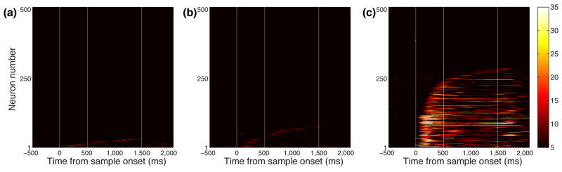
Percentage of explained variance (PEV) across time for all neurons calculated using a sliding ANOVA. Each row represents the PEV of a single neuron. Neurons are sorted based on the time they show a significant PEV. Vertical white lines indicate the onset of the sample stimulus, the beginning of the delay and the onset of the test stimulus. The PEV on one-item trials that is attributable to the color of the item, when colors are either (a) assessed independently or (b) grouped. (c) The PEV attributable to the location of the item on one-item trials.
In contrast to the low incidence of neurons encoding the color of the item, many neurons (286/507 or 56%) encoded its location (Fig. 3c). To ensure that the low number of color-selective neurons we observed was not due to the fact that on some trials the item appeared in a non-optimal location, we repeated our analysis, but this time restricting it to those trials where the item was in the neuron's preferred location and again using the grouped colors. This did not appreciably increase the incidence of color selectivity (45/507 color-selective neurons or 9%, Supplementary Fig. 3b). Another explanation for the low incidence of color-selective neurons might be that we did not record from the appropriate area of PFC. To ensure that this was not the case, we recorded from many other areas of PFC including dorsolateral PFC, orbitofrontal cortex and the frontal eye fields (Supplementary Fig. 4). There was no evidence that any of these areas had a larger incidence of color-selective neurons than ventrolateral PFC. Thus, despite surveying a large area of PFC, only a very small percentage of neurons in the PFC encoded color information in working memory.
We next used a dimensionality reduction technique, de-mixed Principal Component Analysis or dPCA 20, to examine whether color was encoded in the pattern of firing across the population of recorded PFC neurons. This technique, like PCA, transforms high dimensional data into a more tractable, lower dimensional representation where the first few dimensions (principal components) are the most informative (capture the most variance in the neuronal population's firing rate). However, dPCA also considers the relationships between experimental parameters in order to segregate the proportion of variance attributable to different parameters. The projections of the data into the top 16 dPCs, which captured around 60% of the total variance in the population, are shown in Fig. 4. found that, consistent with previous observations 21, time had the largest influence on the variance of PFC firing rates; 13 of the top 16 components were dominated by time, either on its own or in conjunction with the location parameter. The strong time-dependent modulation of firing rate, that is independent of other experimental parameters, can be seen in the four most informative dimensions (Fig. 4a-d). The location of the stimulus was also strongly encoded. Three of the top 16 dPCs, were dominated by location and accounted for 24% of the variance. Two of these three location dPCs encoded whether the stimulus appeared in either the upper or lower half of the display (Fig. 4e) or on the left or right (Fig. 4g). In addition, some projections showed an interaction of time and location, encoding a different subset of locations during the sample and delay, such as Fig. 4h. Notably, none of the top 16 dPCs were dominated by color. In fact, color only accounted for 0.5% of the variance (Fig. 5).
Figure 4.

(a-p). Projections of the 507 neurons into the top 16 dPCs for one-item trials. The color of the lines represents the location of the item during the sample period; the different shades of the colors represent the color of the item. Colors were grouped into four groups as in the previous analysis (Figure 3b). Vertical lines indicate the onset of the sample stimulus, the delay and the test stimulus.
Figure 5.

Relative contribution of time, item color, item location and non-linear mixtures of these parameters to the variance in the population's firing rates for one-item trials to each principal component. Only the top 16 dPCs are shown.
Finally, we determined the amount of information that we could decode about color or space using a correlation based linear classifier approach, which has recently been used to examine PFC neural encoding 22, 23. The results from this analysis were similar to those from the dPCA analysis. We were able to decode spatial information robustly throughout the trial and at a level approaching 100% accuracy during the sample epoch (Supplementary Fig. 5). In contrast, we could barely decode any information about color: it briefly exceeded chance during the sample epoch and returned to chance levels throughout the delay.
In summary, there was no evidence that PFC encoded the color of the stimulus, either at the single neuron or population level, despite the fact that this was the critical requirement of the task. Instead, neurons encoded the item's location.
Control processes underlying multi-item working memory
The strong encoding of spatial information in PFC neurons, as well as the dynamics in firing rate evident both at the single neuron (Fig. 3) and population level (Fig. 4) suggested that PFC was making an important contribution to performance of the task, albeit not in the maintenance of color information in working memory. To determine the nature of this contribution, we examined whether we could predict neuronal firing rates on two-item trials based on the position of the items (as determined by activity on one-item trials) and the subject's spatial attention (as determined by our behavioral measures of covert attention). We performed a sliding multiple-linear regression where we modeled the two-item response (r2) as: r2 = β0 + β1x1 + β2x2 + β3x3. For each two-item trial, we calculated the mean firing rate that was elicited at each of the two positions on one-item trials. The larger of the two firing rates (i.e. the firing rate elicited by the neuron's more preferred location) constituted parameter x1, while the smaller of the two firing rates constituted parameter x2. Parameter x3 coded which of the two items the animal first attended, as indicated by our behavioral measures of covert attention (see above). It was equivalent to x1 – x2 if the animal first attended to the item in the neuron's preferred location, and x2 – x1 if the animal first attended to the item in the neuron's less preferred location. Supplementary Fig. 6 illustrates the coding scheme. The beta associated with parameter x3 would be positive if a neuron's firing rate correlated with the location indicated by our behavioral measure of attention and negative if it correlated with the alternative location. Since we defined the third regressor or with respect to the neuron's location preference, we only analyzed neurons that had a significant spatial preference on the one-item trials. Additionally, because we did not explicitly manipulate where the animal attended, we only performed this analysis using those neurons whose spatial selectivity was not highly co-linear with the location of spatial attention as measured by the variance inflation factor (vif ≤ 2.5). These constraints meant that our analysis was restricted to 258 neurons.
Overall, the model provided a good fit to the neuronal data. Out of the 258 neurons, 215 (83%) were significantly fit by the model (evaluated at p < 0.01). On average, a neuron's one-item response to the preferred item had a stronger on effect its two-item response compared to the less preferred item (Fig. 6a). The response of a neuron on the two-item trials is, at least in part, a weighted sum of the response to the two items when presented individually, with the item in the neuron's preferred location contributing more to the neuron's response then the item in the neuron's less preferred location (Fig. 6b). The slope of the regression line through the population is 0.55 indicating that the item in the neuron's preferred location is approximately twice as important in driving the neuron's response compared to the item in the neuron's less preferred location.
Figure 6.

Standardized beta values from the sliding regression model. (a) Average β1 and β2 values, corresponding to the preferred and non-preferred locations determined from the one item-conditions. (b) Plot of peak β1 vs. peak β2 for all neurons. The neurons preferred location had a larger influence (β1) on the two-item response compared to the less preferred location (β2). The solid black line shows a least squares fit. (c) Pseudo-color plot showing the distribution of β3-values across the population as a function of time. Each column in the plot corresponds to a single distribution of the β3 value for the 215 neurons at that time bin. The color bar indicates the number of neurons that had a particular β-value. Only neurons with a significant β3 were included. The white asterisks indicate time bins for which the distribution of β3 values is significantly different from zero. Average β3 values for (d) the subpopulation of neurons for which the β3-value did not switch sign and (e) for the neurons for which the β3-value did change sign. The red trace denotes the neurons that had an initial positive β3-value while the blue trace indicates those neurons that had an initial negative β3-value. The shaded color region around the traces denotes the s.e.m.
In addition, we found that the two-item response correlated with the locus of spatial attention. This relationship between the two-item response and attention was more complex than the encoding of the spatial location of the items. Neurons were positively as well as negatively correlated with the locus of attention. The neuronal population was initially significantly biased towards a positive correlation, which then switched to a negative correlation (Fig. 6c). This pattern of results could arise for two reasons. One possibility is that there are two populations of neurons, one of which quickly encodes the attended location, the other of which more slowly encodes the other location. Alternatively, there may be a single population in which neural activity initially correlates with the attended location and then shifts to correlate with the other location. To differentiate these possibilities we divided our population into neurons in which the β3-value was maintained across the sample and delay epochs (Fig. 6d, 135/215 neurons) and those in which the sign of the β3-value switched (Fig. 6e, 80/215 neurons), as well as according to whether the neurons initially encoded x3 with a positive or negative relationship, reflecting encoding of the attended or unattended location respectively. For those neurons that maintained the same β3-value, there was no evidence of any difference in the mean time that positive or negative neurons first encoded x3 (positive: 294-ms ± 14-ms, negative: 326-ms ± 19-ms, t-test, t144 = -1.85, p > 0.07). For those neurons that switched the β3-value, there were significantly more positive neurons (53/80) than negative neurons (27/80, binomial test, p < 0.005).
In summary, the spatial information encoded by PFC neurons served multiple functions. The majority of neurons encoded the location of the two items on the screen. We were able to decode this information since it was a linear combination of the neurons' responses to one item. In addition, a substantial population of neurons encoded the subjects' attention. The activity of these neurons initially correlated with the location of the attended item and then correlated with the alternative item, consistent with the subject shifting their attention from one item to the other.
We performed several additional analyses, using variants of our regression model, to examine whether there were other ways to characterize the spatial coding. First, we examined whether there was additional variance in neural firing rates that could contribute to the precision with which information was stored. We captured this by adding a dummy coded parameter that indicated whether the final response of the subject was correct or incorrect. There was little evidence that this parameter was encoded (Supplementary Fig. 7), showing that trial-to-trial variance in the activity of single PFC neurons did not contribute to performance over and above the effects captured by covert attention. Second, we examined the relationship of our model to the biased competition model that has been proposed to account for attentional effects in posterior sensory cortex. Contrary to this model, the encoding of the spatial location of the items did not depend on whether the first attended stimulus was the neuron's preferred or unpreferred stimulus (Supplementary Fig. 8). This supports our original conclusion. PFC spatial signals consist of a static encoding of the spatial location of the stimuli and a dynamic modulation associated with the attentional locus.
Neural signature of working memory load and precision
Studies using magnetoencephalography 24 and event related potentials 12, 14 have shown that oscillatory brain activity in certain frequency bands can predict working memory capacity. To examine whether oscillatory brain activity could predict the precision of working memory representations, we performed a time-frequency decomposition of the local field potentials (LFPs) that we recorded at the same time as our single neuron data. We found clear changes in the power of these signals relative to baseline activity during the performance of our working memory task (Fig. 7). The largest differences in power were concentrated around three different frequency bands: 1–7 Hz (theta), 8–16 Hz (alpha) during the sample epoch, and 20–35 Hz (beta/gamma) during the delay epoch. Thus, we focused our analysis on these frequency bands. We examined whether the power at these frequency bands could predict the precision with which items were maintained in working memory. We focused on the two-item trials since it was here that we expected to see the greatest variance in precision. For each session, we divided the trials into three 500 ms epochs: sample, early and late-delay (first and second halves of the delay period respectively). For each epoch, we calculated the average power in each band on a trial-by-trial basis and split trials into high and low power trials with respect to the median power. We estimated the precision with which the two colors were stored using the same behavioral model as described above but using only high or low-power trials. We normalized these precision values with respect to our precision estimate obtained using data from all trials. The results are shown in Fig. 7c-e. On average, for the lower two frequency bands (theta and alpha), higher LFP power led to more precise working memory representations during both the sample and delay, whereas in the higher frequency band (beta/gamma) the effect was reversed, with precision lower for high-power trials compared to low power trials, and occurred only during the delay.
Figure 7.
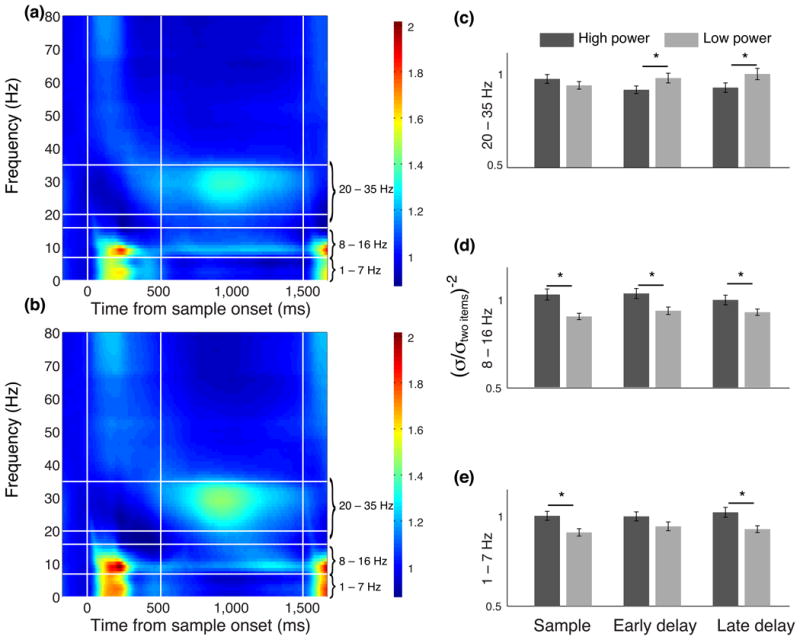
Average time-frequency power spectrum relative to baseline (500-ms before sample onset) for (a) one-item trials and (b) two-item trials. The frequency bands that showed the largest change in power are indicated by the horizontal white lines and are labeled on the right margin of the plots. Vertical lines indicate the times of sample, delay and test onset. (c-e) Normalized precision in three different trial epochs calculated using either high or low power trials in three frequency bands. The asterisks indicate a significant difference between high and low power trials (t-test, p <0.01).
Increased power in the alpha and theta bands has been associated with long-range communication between brain areas 25, 26, and so we hypothesized that, in the current task, it might reflect the mechanism by which PFC maintains color information in posterior sensory cortex. This could be accomplished by using spatial representations to increase the precision of color information at specific locations. If this were the case, we might expect stronger alpha/theta power on those electrodes containing spatially selective neurons. To determine whether this was the case, we first performed a time-frequency decomposition of the LFP signal on each recorded channel. We then averaged this signal across those channels that contained neurons encoding spatial information (the 215 neurons described in Fig. 6) and those channels that did not contain spatially selective neurons. We then subtracted these two signals (spatial – non-spatial). The results of this analysis for one-item and two-item trials are shown in Figs. 8a and 8b respectively. For both kinds of trials, there was a significant alpha/theta power increase on spatial channels relative to non-spatial channels, particularly at the onset of the sample epoch and the onset of the delay epoch. Long-range communication between PFC and posterior sensory cortices may be particularly important during initial processing of the stimuli and initiating their maintenance in working memory.
Figure 8.

Average difference in LFP power between electrodes with spatially selective neurons and electrodes without spatially selective neurons. Data are shown separately for a) one-item trials and b) two-item trials. Black stippling denotes the points where the difference is significant (permutation test, p < 0.01).
Discussion
Several theories argue that an important PFC function is encoding task relevant information 22, 27. In the current task, the most important requirement was to maintain information about color, yet this information was not encoded by PFC neurons. Instead, neurons encoded the spatial location of stimuli. These findings are counter to the notion that PFC represents task relevant information and suggest that spatial information is potentially a key feature around which PFC control signals are organized.
Storing precise sensory representations in working memory
Our results contrast with a recent study by Buschman and colleagues, which reported many PFC neurons encoding color during a working memory task 15. There are several methodological differences that might account for this. The Buschman study used a small set of six colors, which were selected to be highly discriminable from one another and were not isoluminant, and at any given spatial position only one of two colors was possible (Buschman, personal communication). In contrast, we used a larger set of colors that covered a circular, isoluminant space, any color could appear at any spatial position, and there was a range of color changes at test, some of which were relatively subtle. Thus, the Buschman task could be solved in a categorical manner by assigning stimuli to broad categories of color and then detecting whether there was a change, consistent with previous research that PFC neurons can encode arbitrary categories in working memory 28, whereas our task required a precise representation of color. These distinctions make sense from a computational perspective. A principal function of sensory cortex is discrimination: enabling one to perceive subtle differences between stimuli. In contrast, a principal function of PFC is categorization and abstraction which involves ignoring subtle differences between stimuli as irrelevant. Thus, our task favors neural representations of color in sensory cortex while the Bushman task favors PFC. This division of labor makes sense since the alternative would require PFC to replicate in frontal cortex all of the computational capabilities of sensory cortices in terms of representing sensory information.
Similar ideas have been proposed by human neuroimaging studies using multivariate pattern analysis to decode where information is stored during working memory. These studies suggest that information is stored in posterior sensory cortex rather than PFC 29-31. Indeed, whether information is stored in sensory cortex or PFC can depend upon task demands. If subjects are required to remember sensory information then information is stored in sensory cortex, whereas if they must maintain category information, it is stored in PFC 32. These findings can also be explained by the precision of sensory information required by the task. When a precise sensory representation is required information is stored in sensory cortex, but when information is abstract and requires a less precise sensory representation information is stored in PFC. Thus, there is agreement between our findings and those from human neuroimaging. Furthermore, our results show that negative results in PFC in neuroimaging studies are not simply artifacts of the decoding procedure or the BOLD signal. Even at the level of single PFC neurons, there was no evidence that PFC neurons were encoding precise sensory representations in working memory.
One task that did require a precise representation of the memoranda is the vibrotactile discrimination task of Romo and colleagues 33. Monkeys reported whether the second of two sequentially presented vibrotactile stimuli was of higher or lower frequency than the first. PFC neurons precisely encoded the frequency of the first stimulus in working memory until the delivery of the second stimulus, potentially challenging our ideas. However, the observed neural responses (monotonic encoding) do not unambiguously relate to the memorandum. They could reflect the probability that the subject is going to report whether the first stimulus was higher or lower than the second. If the first stimulus is of low frequency it is more likely the subject will be selecting the ‘lower’ response, while the opposite is true if the first stimulus is of high frequency. Such encoding is not outlandish. For example, PFC neurons encode the confidence of an animal in its response with a very precise monotonic relationship 34. Furthermore, this interpretation could explain why ‘working memory’ activity in the vibrotactile discrimination task was stronger in premotor cortex than PFC: the neural firing rate relates more to the preparation of a particular response than working memory per se 35. Our task avoids these issues, because the sensory space was circular and so subjects could not infer anything about the test stimulus from the sample stimuli.
There are two other explanations that might account for a lack of color encoding. First, a confound in much PFC research is task difficulty: more difficult tasks reliably activate PFC 36, so a lack of PFC activity could reflect an easy task. However, our task was very challenging for the subjects, pushing their limits perceptually (the difficulty of the color discrimination) and cognitively (the number of items that had to be remembered). Thus, we have a surprising result on two counts: a lack of PFC encoding for a key behavioral variable during the performance of a challenging task. Second, it may be that color working memory is restricted to a small specialized patch of PFC. Neuroimaging data have suggested a modular organization within monkey PFC for face processing 37 and color might conceivably be similarly organized.
Controlling the allocation of cognitive resources
Although PFC neurons did not encode color information, they were not silent during performance of our task. The spatial location of items was strongly encoded, as was a signal correlating with subjects' covert attention. An important question is what function these signals serve. They could be a top-down attentional signal that helps prioritize processing to certain items in the visual field. In support of this, subjects' performance was better for the item whose location correlated with our behavioral and neural measures of covert attention. Neuroimaging studies have observed spatially topographic representations in PFC 38, 39 and spatial selectivity when top-down attentional control is required 40. Indeed, a recent study using multivariate pattern analysis showed that a region of inferior PFC contained a spatially topographic representation that could be decoded whenever a subject performed either a spatial working memory task or a task requiring shifts of covert spatial attention 41. Our results show that these working memory and attention signals are multiplexed even at the level of single PFC neurons. The contrast between PFC encoding of spatial and color information suggests that they serve qualitatively different roles, consistent with psychophysical and neurophysiological evidence that spatial and feature-based attention are dependent on dissociable mechanisms 42-44.
Our results also suggest a mechanism by which PFC could implement these attentional effects on information in posterior sensory cortex. The precision with which information was stored in working memory correlated with increased power in theta and alpha bands of the LFP, and decreased power in beta and gamma bands. Synchrony in theta and alpha is associated with long-range communication between brain areas, whereas synchrony in higher frequencies is associated with local processing 25. Thus, increased working memory precision is associated with increased long-range processing, consistent with the notion that PFC is controlling the representation of information in posterior sensory cortex, rather than storing that information itself. Indeed, neurophysiological recordings have shown increased theta and alpha synchrony in frontal cortex and posterior sensory cortex during working memory tasks 25, 26, 45, 46, and increased synchrony in these areas correlates with increased working memory capacity 24, 46. More generally, it has been proposed that theta acts as a carrier frequency for top-down control. Theta-gamma coupling has been observed between different cortical areas across a range of cognitive tasks 47. Increased theta has been seen in human cortex when attention is shifted 48 and increased theta-gamma coupling is seen in human hippocampus when multiple items must be held in working memory 49. In addition, in rats, theta coherence between hippocampus and PFC is seen when an animal makes a choice, with increasing coherence producing more precise neural representations of task-relevant information 50.
In sum, the increased alpha/theta we observed in PFC might by a mechanism that could co-ordinate communication between PFC and either the hippocampus and/or posterior sensory areas and enable PFC to influence the precision with which information is stored in working memory. These ideas are necessarily speculative since we only recorded from PFC, but future studies could directly test these hypotheses by simultaneously recording from PFC, posterior sensory cortex and the hippocampus. We did look for evidence of theta-gamma coupling within PFC, but found little of note, although this is perhaps not surprising as cross-frequency coupling tends to be observed between brain areas.
Conclusion
Our results pose a challenge for some of the dominant theories of PFC function. In a task requiring subjects to hold color information in working memory, there was little evidence that PFC neurons encoded color. Thus, the notion that PFC neurons encode all types of task relevant information needs to be modified. PFC neurons do not appear capable of maintaining precise sensory representations in working memory, and may only encode sensory information when a coarse representation suffices for task performance (such as when highly discriminable stimuli are used) or when the stimuli can be represented at an abstract, conceptual level. In contrast, we found that the majority of PFC neurons encoded spatial signals and that these signals correlated with the position of the items on the screen as well as the subjects' attention to those items. These signals could be used to selectively improve the precision of specific sensory representations, coordinated via increased synchrony in the theta and alpha bands between PFC and posterior sensory cortex.
Materials and methods
Subjects
Subjects were two male rhesus monkeys (Maccaca mulatta) aged 4 to 5 years and weighing 11 to 13 kg at the time of the experiment. Subjects' fluid intake was regulated in order to maintain motivation to perform the task. During testing subjects sat in a primate chair facing a 19-inch LCD computer screen placed at a distance of 32-cm. A pair of computers running NIMH Cortex (http://dally.nimh.nih.gov) controlled the timing and presentation of stimuli. All procedures were in accord with the National Institute of Health guidelines and the recommendations of the U.C. Berkeley Animal Care and Use Committee.
Multiple item change detection task
Subjects were trained on a color change detection task adapted from the human literature 51, illustrated in Fig. 1. At the start of the trial a fixation square (0.5° × 0.5° of visual angle) appeared in the center of the screen. Subjects had to maintain their gaze within 1.1° of the fixation spot for 800-ms. Subsequently, a sample array of 1 or 2 different colored squares appeared on the screen for 500-ms. At the end of the sample period, the array disappeared and there was a delay of 1000-ms during which subjects had to keep the color of the squares in visual working memory. At the end of the delay, one of the squares in the array was presented again and subjects had to indicate, using a lever, whether the color at that location had changed (move lever down) or remained the same (move lever up). Subjects were free to respond as soon as the test square appeared on the screen. Correct responses were rewarded with 0.5-ml of juice. Incorrect responses were discouraged with a 4-s timeout. If subjects broke fixation at any time prior to their response, the trial was aborted, the entire screen turned red for 10-s and a new trial was started. There was a 3-s inter-trial interval.
Stimuli were squares 3.5° × 3.5° of visual angle presented in any of four fixed locations 5° away from fixation on a black background. Colors were chosen from the 1976 CIE L a* b* color space. We fixed the luminance at L = 70 and varied the a* and b* parameters to produce 20 different colored squares arranged circularly. All 20 colors were used as sample and test colors. We restricted, however, the distances between sample and test colors (ΔE) to the set ΔE ∈ (0, 40, 50, 60, 70, 80, 90, 100). As a point of reference, adjacent colors in the color circle shown in Fig. 1 are separated by 17 units from each other. Additionally, for two item trials, in order to prevent any potential confusion, the colors of the squares in the array were chosen such that the distance between them was at least 30 units.
Neuronal recordings
We recorded single units simultaneously from PFC using arrays of 8-32 tungsten microelectrodes. We randomly sampled neurons; no attempt was made to select neurons based on responsiveness. This procedure ensured an unbiased estimate of neuronal activity. To determine the number of neurons required to detect color encoding, we performed a power analysis and determined that for a desired power of 0.8 and an alpha level of 0.05 we needed to record from at least 26 neurons. Typically around 30% of PFC cells show selectivity in any given experiment, thus our required sample size is least 87 cells. Ideally we aim to replicate our results in a second monkey thus we require a total of at least 174 cells.
All recording and preprocessing of neural activity was performed prior to analyzing neural encoding. Data collection and subsequent analysis were automated, however they were not blind to the experimental conditions. Waveforms were digitized and analyzed offline. Our recording techniques are described in more detail elsewhere 52.
Analytical Methods
Modeling behavioral performance with a variable precision model
We have previously modeled subjects' performance on the color change detection task. We fit a variety of models to our data, including those in which working memory capacity was modeled as a fixed number of slots, but we found that the best fit was provided by models that characterized working memory as a resource to be shared among the stored items 17. To estimate the precision of representations in working memory we calculated the probability of subjects detecting a change in color as a function of distance between sample and test colors. This probability is modeled by 53:
| (1) |
where Φ is the cumulative distribution function of a normal distribution with mean μ and variance σ2 . Equation 1 assumes that subjects have a noisy representation of the sample stimulus in working memory and they will respond ‘change’ whenever the difference between the test stimulus and the working memory representation exceeds a criterion given by μ. In addition, we incorporated a guessing parameter g into this model to account for the fact that on some proportion of trials subjects might fail to detect a change for reasons unrelated to the precision of the working memory representation, for example, due to a lack of motivation or a failure to attend to the stimuli, and instead guess that a change has occurred. On a certain proportion of trials, g, the subject randomly guesses, while on the remaining proportion of trials, 1 - g, the subject's behavior can be described by the model given by Equation 1. In addition, we added a bias parameter, b. One might expect the animal's guesses to be randomly distributed between the ‘change’ and ‘no change’ responses, but this is not necessarily the case. The subject could favor one or other response when they are not sure of the correct response and the bias parameter captures this. Thus, the complete model was:
| (2) |
In other words, the relationship between the probability of detecting a change as the size of the change increases is well fit by a logistic function. The precision with which the animal has stored the sample stimulus in working memory determines the slope of the logistic function: the noisier the representation the more frequently the animal chooses the incorrect response. The guessing parameter controls the asymptote of the logistic function. If the difference between the test stimulus and sample stimulus was sufficiently large, the asymptote should be 1: with a sufficiently large change the subject always reports a change. However, factors such as lack of motivation or attention could prevent this. Even with a very large change between test and sample, the animal may sometimes report that there was no change, and so the asymptote would be less than 1. Note that the asymptote of the logistic function is varying for reasons that are independent of its slope. The bias term controls the y-position of the logistic, capturing whether choices are equally distributed between ‘change’ and ‘no change’.
We fit the model for one-item and two-item trials separately and estimated the precision of stored representations as 1/σ2. We then examined how neural signals correlated with this estimate of precision.
Behavioral index of covert attention
For each two-item trial, we found the microsaccade direction as described in Supplementary Fig. 1. Separately, for each session and each two-item configuration, we calculated the median RT when the test item appeared at either of the two locations. We defined the location for which the median RT was fastest as the behaviorally preferred location and the location for which the median RT was slowest as the unpreferred location. We then classified the attentional bias for each trial, by determining whether the RT for that trial was closer to the median RT for the preferred or unpreferred location. This provided us with two separate estimates of the attended location for each trial, one based on the microsaccade and one based on the RT. There was good agreement between the two estimates as measured using Fleiss' Kappa, a measure of agreement between classes assigned by two or more classifiers that ranges from 0 (no agreement) to 1 (perfect agreement). The two estimates showed significant agreement for 68 out of 78 (87%) recording sessions. Each estimate had its advantages and disadvantages. The microsaccade estimate was unambiguous, but was not present on all trials. In contrast, the RT estimate was noisier, but was present on every trial. Therefore, to get a more robust estimate we combined them. From this combined measure we determined which location was most frequently classed as attended. For example, consider the configuration shown in Supplementary Fig. 1, with items in the upper-right (U) and lower-left (L). Suppose we had 5 trials with this configuration and for each trial the microsaccade measure gave ms = [U L U U U] and the RT measure gave rt = [U U L U U]. We pooled the measures and obtained pooled = [ms rt] = [U L U U U U U L U U]. Thus, for this configuration, U was the most common pooled location and so for these five trials we assigned the upper-right as the attended location.
Single neuron selectivity for one-item trials
To quantify neuronal selectivity in the one-item trials we performed a sliding two-way ANOVA on the neuron's average firing rate using the color and spatial location of the sample as factors. We used a 200-ms window that we shifted in 20-ms steps across the duration of the trial. We defined a selective neuron as one where p < 0.005 for three consecutive time bins at any point in the trial. We ensured that this criterion was reasonable by assessing the false discovery rate, which we determined by calculating the proportion of neurons that reached criterion during the fixation period, before the subject had any information about the color and position of the sample stimuli. Our criterion yielded 4.93% of selective neurons during the fixation period, which was an acceptable false discovery rate. To quantify the amount of information that a neuron encoded about each factor, we used the sliding two-way ANOVA to calculate the percentage of explained variance (PEV) in the neuron's firing rate that could be attributed to color or space: PEVfactor = SSfactor/SStotal, where SS indicates the sum of squares.
Population response for one-item trials
We used a recently developed dimensionality reduction technique called demixed Principal Components Analysis (dPCA) to look for the common firing patterns present in our population of neurons. Demixed PCA is similar to PCA in that it finds the dimensions of the data that account for the most variance. However, dPCA also minimizes the number of parameters that contributes to each component. Thus, each principal component (or dimension) depends on the least possible number of parameters (see 20 for a full theoretical account of this method). Briefly, for all neurons we calculated firing rate by counting the number of spikes in non-overlapping 20-ms time bins for each combination of parameters (also referred as a condition) and constructed an N x c x t matrix of responses (Y) where N is the number of neurons, c represents the different conditions and t represents time. Each condition was comprised of all the trials in which a certain color appeared at a certain location. For this analysis, we used the same color grouping that maximized the PEVcolor as described in Supplementary Fig. 2. Thus, we end up with a total of 4 spatial locations and 4 color groups for a total of 4 × 4 = 16 conditions. The goal of dPCA is to find the projection of Y that maximizes the amount of variance captured while at the same time depending on the least number of parameters. This is achieved by parceling out the overall variance of Y into separate parts that capture the variance due to different parameters. A modified Expectation-Maximization algorithm is then used to maximize the variance captured by the smallest possible number of parameters or mixtures of parameters.
Single neuron response to two-item trials
We performed a sliding regression for the two-item trials with a 200-ms window and 20-ms steps to model a single neuron's response to the presentation of two-items using its activity on the one-item trials. Our model was of the form: r2 = β0 + β1x1 + β2x2 + β3x3, where r2 is the neuron's average firing rate during each two-item trial, x1 and x2 are the mean responses to the more and less-preferred locations respectively on the one-item trials and x3 is a regressor that accounts for the locus of covert attention with respect to the neuron's spatial preference. Specifically, for each two-item trial, if attention was directed to a neuron's more preferred location (relative to the other possible locations on the screen) the trial was coded as x3 = x1 – x2. Alternatively, if attention was directed to the neuron's less preferred location the trial was coded as x3 = x2 – x1. See Supplementary Fig. 6 for an illustration of this coding scheme.
Local field potential analysis
LFPs were collected with a sampling frequency of 1-kHz and analyzed offline. Data were band-pass filtered in the range 0 -100 Hz and we calculated spectrograms using a multi-taper spectral estimation method from the Chronux toolbox (chronux.org) using tapers N = 5 and a time-bandwidth product W = 3. These parameters control the smoothing of the spectrogram in time and frequency. Data from one-item and two-item trials were averaged separately to calculate the spectrograms. We visually examined spectra from all channels and heuristically determined the frequency bands of interest based on the frequencies that showed the clearest change in power relative to baseline during the performance of the task (Fig. 7).
Supplementary Material
Supplementary Figure 1. Behavioral measures of covert attention. We analyzed subjects' eye movements and were able to detect microsaccades made during the sample period. We used the filtered eye speed to determine the occurrence and direction of the microsaccades. We used a threshold crossing detection algorithm that detected when the eye speed exceeded two standard deviations of the eye speed during the initial fixation (when no visual stimuli were present on the display). (a) Example of a single trial where items were presented in the upper right and lower left locations. The animal makes a microsaccade towards the upper right item during the sample period (red trace). For this trial, the test item appeared in the lower left and the animal made a full saccade toward that location after he was no longer required to hold fixation (green trace). (b) Eye speed during the course of the trial. During the sample period, there is a small, brief increase in speed corresponding to the microsaccade. The blue triangle indicates the time when the animal made his response and the large peaks in speed correspond to a saccade to the test item. (c) Pattern of microsaccades for all trials in this session. Each plot illustrates a specific two-item configuration, with the position of the items indicated by the gray squares. Red arrows indicate the angular direction of the first microsaccade. The blue lines indicate the angular direction of the second microsaccade (if there was one). There was a clear pattern evident. The subject favored microsaccades to the top left item. If no item was present in the top left, he favored microsaccades to the top right, and if there no items on the top of the screen he favored microsaccades to the bottom left. Such a pattern was consistent with the subject covertly attending to the items, starting with the item in the top right and moving counter-clockwise through the items. Similar stereotyped patterns of covert attention have also been reported in monkeys performing visual search tasks. Note that microsaccades were only made during the sample epoch; they were absent during the delay. Thus, we cannot be sure how attention was allocated during the delay period.
Supplementary Figure 2. Color grouping procedure. In order to give the sliding-ANOVA analysis the greatest chance of detecting color-related information, we grouped the 20 colors in the four groups of five colors per group. For each neuron, we grouped colors in four groups of five colors per group (a) and calculated the amount of information encoded by the neuron using the percentage of explained variance (PEV) measure. (b) We changed the colors that comprised each group by rotating the group boundaries clockwise by one color and calculated the PEV once more. (c) We repeated this procedure until we had traversed all the color space. The false discovery rate for this procedure, calculated by assessing the proportion of neurons that reached the criterion during the fixation period, was 4.9%.
Supplementary Figure 3. Additional color selectivity measures. (a) To examine whether neural responses to colors could be fit by a von Mises distribution we performed a linear regression that was modified for circular data: r = β0 + β1sinθ + β2cosθ, where r is the neuron's firing rate, and θ is the angle of the color in our color space (Figure 1). The plot shows the percentage of variance in neuronal firing rates that could be explained by the model for each neuron at each point in the trial. Each row represents the selectivity a single neuron and neurons are sorted based on the time they show significant color selectivity. Vertical white lines indicate the onset of the sample stimulus, the beginning of the delay and the onset of the test stimulus. We defined a neuron to be color tuned if the regression model significantly fit the data for three consecutive time bins. Using this criterion we found that only 13% (65/507) of neurons were color-tuned. Similar to our sliding PEV analysis, in order to correct for multiple comparisons, we calculated the number of neurons for which the p-value of the regression was larger than 0.005 for three consecutive time bins during the fixation period. This resulted in a false discovery rate of 4.3%. (b) To examine whether the incidence of color selectivity depended on the spatial tuning of the neuron, we restricted our sliding ANOVA analysis (as described in Supplementary Figure 2) to trials in which the color was shown in each neuron's preferred location. Color tuning remained evident in only a small minority of neurons (45/507 or 9% of neurons). Thus, despite using a variety of analysis methods, PFC neurons consistently showed little encoding of color.
Supplementary Figure 4. Recording Locations. To ensure that the lack of color encoding in PFC was not due to the fact that we had confined our recordings to the ventrolateral PFC, we extended our recordings in to the dorsolateral prefrontal cortex, orbitofrontal cortex and the frontal eye fields. The plots show flattened cortical representations illustrating recording locations from the two subjects, and the proportion of color-selective neurons in each location (as indicated by the color of each data point). Gray shading indicates the position of a sulcus. The anterior–posterior (AP) position is measured relative to the interaural line. The circle dashed line demarcates the recording locations of the neurons in the main analysis. Despite recording an additional 323 neurons from these areas, we did not see a significant number of color-selective neurons.
Supplementary Figure 5. Decoding of spatial and color information using a linear classifier. We used a neural-population decoding algorithm that uses a maximum correlation classifier to classify multivariate patterns of activity across the population. By determining how accurately the classifier predicts which experimental conditions are present, one can determine how much information about the experimental conditions is encoded by the neuronal population. We focused our analysis on the single item trials and we decoded the location and the grouped color (see Supplementary Figure 2) of the items using the entire population of PFC neurons. The decoding algorithm used a cross-validation procedure in which the data was randomly split into 10 separate subsets. Nine of these subsets were used to train the classifier and the remaining set was used as a testing set. This cross-validation procedure was repeated 10 times to ensure that each set was used as part of the training and testing sets at least once. This generated 10 classification estimates, which were then averaged to obtain a more robust single classification estimate. This whole procedure was repeated 20 times, each time randomly selecting different subsets of training and testing sets. The results from the 20 repetitions were then averaged and are shown separately for (a) location and (b) color decoding. Shading indicates the standard error of the mean for the 20 separate repetitions of the decoding scheme. The horizontal line at 25% indicates chance performance. Vertical lines indicate the onset of the sample, delay and test epochs, respectively. The results from this decoding analysis strongly support the results from the demixed PCA analysis. We were able to decode spatial information robustly throughout the trial and at a level approaching 100% accuracy during the sample epoch (chance performance was 25%). In contrast, we could barely decode any information about color: it briefly exceeded chance during the sample epoch and returned to chance levels throughout the delay.
Supplementary Figure 6. Two item regression coding scheme. Illustration of how the x3 regressor was determined. (a) Spike density histogram showing the firing rate of a single neuron for each of the four locations during the one-item trials. The color of the line corresponds to the location indicated by the legend. This neuron responded strongest to item in the lower left and weakest to items in the upper right. Vertical lines denote the time when the item was presented on the screen. (b) Response to single items presented at the four locations for a different neuron. This neuron responded more to items on the left. (c) Schematic of a two-item trial. In this trial items were presented in the upper and lower left. Using our behavioral estimate of attention, we determined that for this trial the subject first shifted attention to the item in the upper left (denoted by the gray circle). When these items were presented in isolation, the neuron in (a) fired with an average peak rate of 17-Hz to the item in the upper left location (blue trace) and 42-Hz to the item in the lower left (green trace). Thus, x1 = 42 and x2 = 17. The attended location was the neuron's less preferred location of the two and so x3 = x2 – x1 = (17 – 46) = -29. The neuron in (b) had a peak one-item response to items on the upper left that was higher (x1 = 19) than the one-item response to items on the lower left (x2 = 9). Thus, attention was directed to the neuron's more preferred location, and so we would say that x3 = x1 – x2 or (19 - 9) = 10. The upshot of this coding scheme is that the beta for x3 will be positive when the neuron's firing rate correlates with the location indicated by our behavioral indices of covert attention and negative when the neuron's firing rate correlates with the alternative location.
Supplementary Figure 7. Regression model with outcome and response parameters. To examine whether there was any additional variance in the firing rate of individual neurons (over and above the information we had already decoded about space) that could predict whether or not the animal would correctly detect the change in color we added two additional parameters to the regression model: whether firing rate predicted the subject's response (‘change’ or ‘no change’) and the subject's performance (trial outcome: correct or incorrect). (a) β values for all neurons corresponding to the preferred location, non-preferred location, trial outcome and subject's response respectively. There was virtually no variance explained by either response or outcome until the test epoch. (b) and (c) show the β3 values separated according to whether the initial β3-value was positive or negative and whether the β3-value switched sign (b) or stayed constant through the trial (c). The regression was performed on spikes aligned to the onset of the sample up to 600-ms before subjects made their response (shown on the left hand side of the plot from time -500-ms to 2100-ms); and using spikes aligned to the time when animals made their response until 500-ms after the response (shown on the right hand side of the panel). Vertical lines indicate onset of the sample, delay and test epochs and the subjects' behavioral response, respectively. Only trials with a reaction time >600-ms were used in this analysis to avoid contamination of response related activity with test-epoch related activity. In practice, this excluded <1% of trials. We also note that this analysis does not necessarily contradict the fact that we were able to detect an effect on the precision of stored information in the local field potential of those electrodes containing spatially selective neurons (Figure 7d, 7e 8). First, the LFP averages activity across many thousands of neurons and so may be more sensitive at detecting the effect of PFC neuronal firing on behavior. More importantly, however, the single neuron firing rate and the LFP are not necessarily directly related to one another. It is the timing of spikes relative to one another that increases the power of the LFP, not their overall rate. Thus, the firing rate of PFC neurons could remain unchanged, and yet the increase in coherence in spikes communicating with posterior sensory areas would give rise to increased power in certain frequency bands of the LFP.
Supplementary Figure 8. Regression model without the attention parameter. The mathematical formulation of the biased competition model is that a neuron's response to two items is the sum of the response to either item presented alone, weighted according to which item is currently being attended. To directly test whether this model predicted PFC neuronal responses, we removed the attention parameter from our original model (β3), sorted the trials according to whether the first attended stimulus was the neuron's (a) preferred or (b) unpreferred stimulus (i.e. whether β3 would have been positive or negative) and then examined the dynamics of β1 and β2. If the biased competition model were applicable to PFC, then β1 should be greater than β2 when the first attended stimulus is the neuron's preferred stimulus. In other words, the neuron's firing rate to the two item trials should be better predicted by the response to the preferred stimulus alone when the subject is attending to the preferred stimulus. In contrast, β2 should be greater than β1 when the first attended stimulus is the neuron's unpreferred stimulus. In other words, the neuron's firing rate to the two item trials should be better predicted by the response to the unpreferred stimulus alone when the subject is attending to the unpreferred stimulus. In fact, β1 and β2 encoding did not depend on whether the first attended stimulus was the neuron's preferred or unpreferred stimulus. This supports our original conclusion. PFC spatial signals consist of a static encoding of the spatial location of the stimuli and a dynamic modulation associated with the attentional locus. These findings are consistent with recent studies of attentional effects in PFC, which have emphasized dynamic modulation of spatial selectivity that does not necessarily reflect the original receptive field. For example, analysis of PFC activity at the population level during visual search shows that there is a rapid global allocation of resources to the target that is largely independent of whether the target is in the neuron's preferred or unpreferred location 5. Similarly, analysis of single neurons in the frontal eye fields have shown that there is a dynamic increase in neural activity that correlates with the locus of attention and is largely independent of the neuron's receptive field 1. Thus, PFC attentional mechanisms are distinct from those in earlier visual areas.
Acknowledgments
The project was funded by NIDA grant R01DA19028 and NINDS grant P01NS040813 to J.D.W. A.H.L. designed the experiment, collected and analyzed the data and wrote the manuscript. J.D.W. supervised the project and edited the manuscript.
Footnotes
The authors have no competing interests.
References
- 1.Constantinidis C, Franowicz MN, Goldman-Rakic PS. The sensory nature of mnemonic representation in the primate prefrontal cortex. Nat Neurosci. 2001;4:311–316. doi: 10.1038/85179. [DOI] [PubMed] [Google Scholar]
- 2.Funahashi S, Chafee MV, Goldman-Rakic PS. Prefrontal neuronal activity in rhesus monkeys performing a delayed anti-saccade task. Nature. 1993;365:753–756. doi: 10.1038/365753a0. [DOI] [PubMed] [Google Scholar]
- 3.Rao SC, Rainer G, Miller EK. Integration of what and where in the primate prefrontal cortex. Science. 1997;276:821–824. doi: 10.1126/science.276.5313.821. [DOI] [PubMed] [Google Scholar]
- 4.Asaad WF, Rainer G, Miller EK. Task-specific neural activity in the primate prefrontal cortex. J Neurophysiol. 2000;84:451–459. doi: 10.1152/jn.2000.84.1.451. [DOI] [PubMed] [Google Scholar]
- 5.Cowan N. The magical number 4 in short-term memory: a reconsideration of mental storage capacity. Behav Brain Sci. 2001;24:87–114. doi: 10.1017/s0140525x01003922. discussion 114-185. [DOI] [PubMed] [Google Scholar]
- 6.Engle RW, Tuholski SW, Laughlin JE, Conway AR. Working memory, short-term memory, and general fluid intelligence: a latent-variable approach. J Exp Psychol Gen. 1999;128:309–331. doi: 10.1037//0096-3445.128.3.309. [DOI] [PubMed] [Google Scholar]
- 7.Conway AR, Kane MJ, Engle RW. Working memory capacity and its relation to general intelligence. Trends in cognitive sciences. 2003;7:547–552. doi: 10.1016/j.tics.2003.10.005. [DOI] [PubMed] [Google Scholar]
- 8.Rouder JN, et al. An assessment of fixed-capacity models of visual working memory. Proc Natl Acad Sci U S A. 2008;105:5975–5979. doi: 10.1073/pnas.0711295105. [DOI] [PMC free article] [PubMed] [Google Scholar]
- 9.Wilken P, Ma WJ. A detection theory account of change detection. J Vis. 2004;4:1120–1135. doi: 10.1167/4.12.11. [DOI] [PubMed] [Google Scholar]
- 10.Zhang W, Luck SJ. Discrete fixed-resolution representations in visual working memory. Nature. 2008;453:233–235. doi: 10.1038/nature06860. [DOI] [PMC free article] [PubMed] [Google Scholar]
- 11.Bays PM, Husain M. Dynamic shifts of limited working memory resources in human vision. Science. 2008;321:851–854. doi: 10.1126/science.1158023. [DOI] [PMC free article] [PubMed] [Google Scholar]
- 12.Vogel EK, Machizawa MG. Neural activity predicts individual differences in visual working memory capacity. Nature. 2004;428:748–751. doi: 10.1038/nature02447. [DOI] [PubMed] [Google Scholar]
- 13.Todd JJ, Marois R. Capacity limit of visual short-term memory in human posterior parietal cortex. Nature. 2004;428:751–754. doi: 10.1038/nature02466. [DOI] [PubMed] [Google Scholar]
- 14.Vogel EK, McCollough AW, Machizawa MG. Neural measures reveal individual differences in controlling access to working memory. Nature. 2005;438:500–503. doi: 10.1038/nature04171. [DOI] [PubMed] [Google Scholar]
- 15.Buschman TJ, Siegel M, Roy JE, Miller EK. Neural substrates of cognitive capacity limitations. Proc Natl Acad Sci U S A. 2011;108:11252–11255. doi: 10.1073/pnas.1104666108. [DOI] [PMC free article] [PubMed] [Google Scholar]
- 16.Siegel M, Warden MR, Miller EK. Phase-dependent neuronal coding of objects in short-term memory. Proc Natl Acad Sci U S A. 2009;106:21341–21346. doi: 10.1073/pnas.0908193106. [DOI] [PMC free article] [PubMed] [Google Scholar]
- 17.Lara AH, Wallis JD. Capacity and precision in an animal model of visual short-term memory. J Vis. 2012;12 doi: 10.1167/12.3.13. [DOI] [PMC free article] [PubMed] [Google Scholar]
- 18.Conway BR, Tsao DY. Color-tuned neurons are spatially clustered according to color preference within alert macaque posterior inferior temporal cortex. Proc Natl Acad Sci U S A. 2009;106:18034–18039. doi: 10.1073/pnas.0810943106. [DOI] [PMC free article] [PubMed] [Google Scholar]
- 19.Gerbella M, Belmalih A, Borra E, Rozzi S, Luppino G. Cortical connections of the macaque caudal ventrolateral prefrontal areas 45A and 45B. Cereb Cortex. 2010;20:141–168. doi: 10.1093/cercor/bhp087. [DOI] [PubMed] [Google Scholar]
- 20.Machens CK. Demixing population activity in higher cortical areas. Frontiers in computational neuroscience. 2010;4:126. doi: 10.3389/fncom.2010.00126. [DOI] [PMC free article] [PubMed] [Google Scholar]
- 21.Machens CK, Romo R, Brody CD. Functional, but not anatomical, separation of “what” and “when” in prefrontal cortex. J Neurosci. 2010;30:350–360. doi: 10.1523/JNEUROSCI.3276-09.2010. [DOI] [PMC free article] [PubMed] [Google Scholar]
- 22.Stokes MG, et al. Dynamic coding for cognitive control in prefrontal cortex. Neuron. 2013;78:364–375. doi: 10.1016/j.neuron.2013.01.039. [DOI] [PMC free article] [PubMed] [Google Scholar]
- 23.Meyers EM, Qi XL, Constantinidis C. Incorporation of new information into prefrontal cortical activity after learning working memory tasks. Proc Natl Acad Sci U S A. 2012;109:4651–4656. doi: 10.1073/pnas.1201022109. [DOI] [PMC free article] [PubMed] [Google Scholar]
- 24.Palva JM, Monto S, Kulashekhar S, Palva S. Neuronal synchrony reveals working memory networks and predicts individual memory capacity. Proc Natl Acad Sci U S A. 2010;107:7580–7585. doi: 10.1073/pnas.0913113107. [DOI] [PMC free article] [PubMed] [Google Scholar]
- 25.von Stein A, Sarnthein J. Different frequencies for different scales of cortical integration: from local gamma to long range alpha/theta synchronization. Int J Psychophysiol. 2000;38:301–313. doi: 10.1016/s0167-8760(00)00172-0. [DOI] [PubMed] [Google Scholar]
- 26.Sauseng P, Klimesch W, Schabus M, Doppelmayr M. Fronto-parietal EEG coherence in theta and upper alpha reflect central executive functions of working memory. Int J Psychophysiol. 2005;57:97–103. doi: 10.1016/j.ijpsycho.2005.03.018. [DOI] [PubMed] [Google Scholar]
- 27.Rigotti M, et al. The importance of mixed selectivity in complex cognitive tasks. Nature. 2013;497:585–590. doi: 10.1038/nature12160. [DOI] [PMC free article] [PubMed] [Google Scholar]
- 28.Cromer JA, Roy JE, Miller EK. Representation of multiple, independent categories in the primate prefrontal cortex. Neuron. 2010;66:796–807. doi: 10.1016/j.neuron.2010.05.005. [DOI] [PMC free article] [PubMed] [Google Scholar]
- 29.Ester EF, Anderson DE, Serences JT, Awh E. A neural measure of precision in visual working memory. J Cogn Neurosci. 2013;25:754–761. doi: 10.1162/jocn_a_00357. [DOI] [PMC free article] [PubMed] [Google Scholar]
- 30.Christophel TB, Hebart MN, Haynes JD. Decoding the contents of visual short-term memory from human visual and parietal cortex. J Neurosci. 2012;32:12983–12989. doi: 10.1523/JNEUROSCI.0184-12.2012. [DOI] [PMC free article] [PubMed] [Google Scholar]
- 31.Emrich SM, Riggall AC, Larocque JJ, Postle BR. Distributed patterns of activity in sensory cortex reflect the precision of multiple items maintained in visual short-term memory. J Neurosci. 2013;33:6516–6523. doi: 10.1523/JNEUROSCI.5732-12.2013. [DOI] [PMC free article] [PubMed] [Google Scholar]
- 32.Lee SH, Kravitz DJ, Baker CI. Goal-dependent dissociation of visual and prefrontal cortices during working memory. Nat Neurosci. 2013;16:997–999. doi: 10.1038/nn.3452. [DOI] [PMC free article] [PubMed] [Google Scholar]
- 33.Romo R, Brody CD, Hernandez A, Lemus L. Neuronal correlates of parametric working memory in the prefrontal cortex. Nature. 1999;399:470–473. doi: 10.1038/20939. [DOI] [PubMed] [Google Scholar]
- 34.Kepecs A, Uchida N, Zariwala HA, Mainen ZF. Neural correlates, computation and behavioural impact of decision confidence. Nature. 2008;455:227–231. doi: 10.1038/nature07200. [DOI] [PubMed] [Google Scholar]
- 35.Hernandez A, et al. Decoding a perceptual decision process across cortex. Neuron. 2010;66:300–314. doi: 10.1016/j.neuron.2010.03.031. [DOI] [PubMed] [Google Scholar]
- 36.Crittenden BM, Duncan J. Task difficulty manipulation reveals multiple demand activity but no frontal lobe hierarchy. Cereb Cortex. 2012 doi: 10.1093/cercor/bhs333. [DOI] [PMC free article] [PubMed] [Google Scholar]
- 37.Tsao DY, Schweers N, Moeller S, Freiwald WA. Patches of face-selective cortex in the macaque frontal lobe. Nature neuroscience. 2008;11:877–879. doi: 10.1038/nn.2158. [DOI] [PMC free article] [PubMed] [Google Scholar]
- 38.Hagler DJ, Jr, Sereno MI. Spatial maps in frontal and prefrontal cortex. Neuroimage. 2006;29:567–577. doi: 10.1016/j.neuroimage.2005.08.058. [DOI] [PubMed] [Google Scholar]
- 39.Kastner S, et al. Topographic maps in human frontal cortex revealed in memory-guided saccade and spatial working-memory tasks. J Neurophysiol. 2007;97:3494–3507. doi: 10.1152/jn.00010.2007. [DOI] [PubMed] [Google Scholar]
- 40.Serences JT, Yantis S. Spatially selective representations of voluntary and stimulus-driven attentional priority in human occipital, parietal, and frontal cortex. Cereb Cortex. 2007;17:284–293. doi: 10.1093/cercor/bhj146. [DOI] [PubMed] [Google Scholar]
- 41.Jerde TA, Merriam EP, Riggall AC, Hedges JH, Curtis CE. Prioritized maps of space in human frontoparietal cortex. J Neurosci. 2012;32:17382–17390. doi: 10.1523/JNEUROSCI.3810-12.2012. [DOI] [PMC free article] [PubMed] [Google Scholar]
- 42.Treisman AM, Gelade G. A feature-integration theory of attention. Cogn Psychol. 1980;12:97–136. doi: 10.1016/0010-0285(80)90005-5. [DOI] [PubMed] [Google Scholar]
- 43.Itti L, Koch C. A saliency-based search mechanism for overt and covert shifts of visual attention. Vision research. 2000;40:1489–1506. doi: 10.1016/s0042-6989(99)00163-7. [DOI] [PubMed] [Google Scholar]
- 44.Wolfe JM. Guided search 2.0: A revised model of visual search. Psychon Bull Rev. 1994;1:202–238. doi: 10.3758/BF03200774. [DOI] [PubMed] [Google Scholar]
- 45.Johnson JS, Sutterer DW, Acheson DJ, Lewis-Peacock JA, Postle BR. Increased alpha-band power during the retention of shapes and shape-location associations in visual short-term memory. Frontiers in psychology. 2011;2:128. doi: 10.3389/fpsyg.2011.00128. [DOI] [PMC free article] [PubMed] [Google Scholar]
- 46.Liebe S, Hoerzer GM, Logothetis NK, Rainer G. Theta coupling between V4 and prefrontal cortex predicts visual short-term memory performance. Nature neuroscience. 2012;15:456–462. S451–452. doi: 10.1038/nn.3038. [DOI] [PubMed] [Google Scholar]
- 47.Canolty RT, et al. High gamma power is phase-locked to theta oscillations in human neocortex. Science. 2006;313:1626–1628. doi: 10.1126/science.1128115. [DOI] [PMC free article] [PubMed] [Google Scholar]
- 48.Daitch AL, et al. Frequency-specific mechanism links human brain networks for spatial attention. Proc Natl Acad Sci U S A. 2013;110:19585–19590. doi: 10.1073/pnas.1307947110. [DOI] [PMC free article] [PubMed] [Google Scholar]
- 49.Axmacher N, et al. Cross-frequency coupling supports multi-item working memory in the human hippocampus. Proc Natl Acad Sci U S A. 2010;107:3228–3233. doi: 10.1073/pnas.0911531107. [DOI] [PMC free article] [PubMed] [Google Scholar]
- 50.Remondes M, Wilson MA. Cingulate-hippocampus coherence and trajectory coding in a sequential choice task. Neuron. 2013;80:1277–1289. doi: 10.1016/j.neuron.2013.08.037. [DOI] [PMC free article] [PubMed] [Google Scholar]
- 51.Luck SJ, Vogel EK. The capacity of visual working memory for features and conjunctions. Nature. 1997;390:279–281. doi: 10.1038/36846. [DOI] [PubMed] [Google Scholar]
- 52.Lara AH, Kennerley SW, Wallis JD. Encoding of gustatory working memory by orbitofrontal neurons. J Neurosci. 2009;29:765–774. doi: 10.1523/JNEUROSCI.4637-08.2009. [DOI] [PMC free article] [PubMed] [Google Scholar]
- 53.Green DM, Swets JA. Signal detection theory and psychophysics. Wiley; New York: 1966. [Google Scholar]
Associated Data
This section collects any data citations, data availability statements, or supplementary materials included in this article.
Supplementary Materials
Supplementary Figure 1. Behavioral measures of covert attention. We analyzed subjects' eye movements and were able to detect microsaccades made during the sample period. We used the filtered eye speed to determine the occurrence and direction of the microsaccades. We used a threshold crossing detection algorithm that detected when the eye speed exceeded two standard deviations of the eye speed during the initial fixation (when no visual stimuli were present on the display). (a) Example of a single trial where items were presented in the upper right and lower left locations. The animal makes a microsaccade towards the upper right item during the sample period (red trace). For this trial, the test item appeared in the lower left and the animal made a full saccade toward that location after he was no longer required to hold fixation (green trace). (b) Eye speed during the course of the trial. During the sample period, there is a small, brief increase in speed corresponding to the microsaccade. The blue triangle indicates the time when the animal made his response and the large peaks in speed correspond to a saccade to the test item. (c) Pattern of microsaccades for all trials in this session. Each plot illustrates a specific two-item configuration, with the position of the items indicated by the gray squares. Red arrows indicate the angular direction of the first microsaccade. The blue lines indicate the angular direction of the second microsaccade (if there was one). There was a clear pattern evident. The subject favored microsaccades to the top left item. If no item was present in the top left, he favored microsaccades to the top right, and if there no items on the top of the screen he favored microsaccades to the bottom left. Such a pattern was consistent with the subject covertly attending to the items, starting with the item in the top right and moving counter-clockwise through the items. Similar stereotyped patterns of covert attention have also been reported in monkeys performing visual search tasks. Note that microsaccades were only made during the sample epoch; they were absent during the delay. Thus, we cannot be sure how attention was allocated during the delay period.
Supplementary Figure 2. Color grouping procedure. In order to give the sliding-ANOVA analysis the greatest chance of detecting color-related information, we grouped the 20 colors in the four groups of five colors per group. For each neuron, we grouped colors in four groups of five colors per group (a) and calculated the amount of information encoded by the neuron using the percentage of explained variance (PEV) measure. (b) We changed the colors that comprised each group by rotating the group boundaries clockwise by one color and calculated the PEV once more. (c) We repeated this procedure until we had traversed all the color space. The false discovery rate for this procedure, calculated by assessing the proportion of neurons that reached the criterion during the fixation period, was 4.9%.
Supplementary Figure 3. Additional color selectivity measures. (a) To examine whether neural responses to colors could be fit by a von Mises distribution we performed a linear regression that was modified for circular data: r = β0 + β1sinθ + β2cosθ, where r is the neuron's firing rate, and θ is the angle of the color in our color space (Figure 1). The plot shows the percentage of variance in neuronal firing rates that could be explained by the model for each neuron at each point in the trial. Each row represents the selectivity a single neuron and neurons are sorted based on the time they show significant color selectivity. Vertical white lines indicate the onset of the sample stimulus, the beginning of the delay and the onset of the test stimulus. We defined a neuron to be color tuned if the regression model significantly fit the data for three consecutive time bins. Using this criterion we found that only 13% (65/507) of neurons were color-tuned. Similar to our sliding PEV analysis, in order to correct for multiple comparisons, we calculated the number of neurons for which the p-value of the regression was larger than 0.005 for three consecutive time bins during the fixation period. This resulted in a false discovery rate of 4.3%. (b) To examine whether the incidence of color selectivity depended on the spatial tuning of the neuron, we restricted our sliding ANOVA analysis (as described in Supplementary Figure 2) to trials in which the color was shown in each neuron's preferred location. Color tuning remained evident in only a small minority of neurons (45/507 or 9% of neurons). Thus, despite using a variety of analysis methods, PFC neurons consistently showed little encoding of color.
Supplementary Figure 4. Recording Locations. To ensure that the lack of color encoding in PFC was not due to the fact that we had confined our recordings to the ventrolateral PFC, we extended our recordings in to the dorsolateral prefrontal cortex, orbitofrontal cortex and the frontal eye fields. The plots show flattened cortical representations illustrating recording locations from the two subjects, and the proportion of color-selective neurons in each location (as indicated by the color of each data point). Gray shading indicates the position of a sulcus. The anterior–posterior (AP) position is measured relative to the interaural line. The circle dashed line demarcates the recording locations of the neurons in the main analysis. Despite recording an additional 323 neurons from these areas, we did not see a significant number of color-selective neurons.
Supplementary Figure 5. Decoding of spatial and color information using a linear classifier. We used a neural-population decoding algorithm that uses a maximum correlation classifier to classify multivariate patterns of activity across the population. By determining how accurately the classifier predicts which experimental conditions are present, one can determine how much information about the experimental conditions is encoded by the neuronal population. We focused our analysis on the single item trials and we decoded the location and the grouped color (see Supplementary Figure 2) of the items using the entire population of PFC neurons. The decoding algorithm used a cross-validation procedure in which the data was randomly split into 10 separate subsets. Nine of these subsets were used to train the classifier and the remaining set was used as a testing set. This cross-validation procedure was repeated 10 times to ensure that each set was used as part of the training and testing sets at least once. This generated 10 classification estimates, which were then averaged to obtain a more robust single classification estimate. This whole procedure was repeated 20 times, each time randomly selecting different subsets of training and testing sets. The results from the 20 repetitions were then averaged and are shown separately for (a) location and (b) color decoding. Shading indicates the standard error of the mean for the 20 separate repetitions of the decoding scheme. The horizontal line at 25% indicates chance performance. Vertical lines indicate the onset of the sample, delay and test epochs, respectively. The results from this decoding analysis strongly support the results from the demixed PCA analysis. We were able to decode spatial information robustly throughout the trial and at a level approaching 100% accuracy during the sample epoch (chance performance was 25%). In contrast, we could barely decode any information about color: it briefly exceeded chance during the sample epoch and returned to chance levels throughout the delay.
Supplementary Figure 6. Two item regression coding scheme. Illustration of how the x3 regressor was determined. (a) Spike density histogram showing the firing rate of a single neuron for each of the four locations during the one-item trials. The color of the line corresponds to the location indicated by the legend. This neuron responded strongest to item in the lower left and weakest to items in the upper right. Vertical lines denote the time when the item was presented on the screen. (b) Response to single items presented at the four locations for a different neuron. This neuron responded more to items on the left. (c) Schematic of a two-item trial. In this trial items were presented in the upper and lower left. Using our behavioral estimate of attention, we determined that for this trial the subject first shifted attention to the item in the upper left (denoted by the gray circle). When these items were presented in isolation, the neuron in (a) fired with an average peak rate of 17-Hz to the item in the upper left location (blue trace) and 42-Hz to the item in the lower left (green trace). Thus, x1 = 42 and x2 = 17. The attended location was the neuron's less preferred location of the two and so x3 = x2 – x1 = (17 – 46) = -29. The neuron in (b) had a peak one-item response to items on the upper left that was higher (x1 = 19) than the one-item response to items on the lower left (x2 = 9). Thus, attention was directed to the neuron's more preferred location, and so we would say that x3 = x1 – x2 or (19 - 9) = 10. The upshot of this coding scheme is that the beta for x3 will be positive when the neuron's firing rate correlates with the location indicated by our behavioral indices of covert attention and negative when the neuron's firing rate correlates with the alternative location.
Supplementary Figure 7. Regression model with outcome and response parameters. To examine whether there was any additional variance in the firing rate of individual neurons (over and above the information we had already decoded about space) that could predict whether or not the animal would correctly detect the change in color we added two additional parameters to the regression model: whether firing rate predicted the subject's response (‘change’ or ‘no change’) and the subject's performance (trial outcome: correct or incorrect). (a) β values for all neurons corresponding to the preferred location, non-preferred location, trial outcome and subject's response respectively. There was virtually no variance explained by either response or outcome until the test epoch. (b) and (c) show the β3 values separated according to whether the initial β3-value was positive or negative and whether the β3-value switched sign (b) or stayed constant through the trial (c). The regression was performed on spikes aligned to the onset of the sample up to 600-ms before subjects made their response (shown on the left hand side of the plot from time -500-ms to 2100-ms); and using spikes aligned to the time when animals made their response until 500-ms after the response (shown on the right hand side of the panel). Vertical lines indicate onset of the sample, delay and test epochs and the subjects' behavioral response, respectively. Only trials with a reaction time >600-ms were used in this analysis to avoid contamination of response related activity with test-epoch related activity. In practice, this excluded <1% of trials. We also note that this analysis does not necessarily contradict the fact that we were able to detect an effect on the precision of stored information in the local field potential of those electrodes containing spatially selective neurons (Figure 7d, 7e 8). First, the LFP averages activity across many thousands of neurons and so may be more sensitive at detecting the effect of PFC neuronal firing on behavior. More importantly, however, the single neuron firing rate and the LFP are not necessarily directly related to one another. It is the timing of spikes relative to one another that increases the power of the LFP, not their overall rate. Thus, the firing rate of PFC neurons could remain unchanged, and yet the increase in coherence in spikes communicating with posterior sensory areas would give rise to increased power in certain frequency bands of the LFP.
Supplementary Figure 8. Regression model without the attention parameter. The mathematical formulation of the biased competition model is that a neuron's response to two items is the sum of the response to either item presented alone, weighted according to which item is currently being attended. To directly test whether this model predicted PFC neuronal responses, we removed the attention parameter from our original model (β3), sorted the trials according to whether the first attended stimulus was the neuron's (a) preferred or (b) unpreferred stimulus (i.e. whether β3 would have been positive or negative) and then examined the dynamics of β1 and β2. If the biased competition model were applicable to PFC, then β1 should be greater than β2 when the first attended stimulus is the neuron's preferred stimulus. In other words, the neuron's firing rate to the two item trials should be better predicted by the response to the preferred stimulus alone when the subject is attending to the preferred stimulus. In contrast, β2 should be greater than β1 when the first attended stimulus is the neuron's unpreferred stimulus. In other words, the neuron's firing rate to the two item trials should be better predicted by the response to the unpreferred stimulus alone when the subject is attending to the unpreferred stimulus. In fact, β1 and β2 encoding did not depend on whether the first attended stimulus was the neuron's preferred or unpreferred stimulus. This supports our original conclusion. PFC spatial signals consist of a static encoding of the spatial location of the stimuli and a dynamic modulation associated with the attentional locus. These findings are consistent with recent studies of attentional effects in PFC, which have emphasized dynamic modulation of spatial selectivity that does not necessarily reflect the original receptive field. For example, analysis of PFC activity at the population level during visual search shows that there is a rapid global allocation of resources to the target that is largely independent of whether the target is in the neuron's preferred or unpreferred location 5. Similarly, analysis of single neurons in the frontal eye fields have shown that there is a dynamic increase in neural activity that correlates with the locus of attention and is largely independent of the neuron's receptive field 1. Thus, PFC attentional mechanisms are distinct from those in earlier visual areas.