Simulations of the role of water in the protein-folding mechanism

Abstract

There are many unresolved questions regarding the role of water in protein folding. Does water merely induce hydrophobic forces, or does the discrete nature of water play a structural role in folding? Are the nonadditive aspects of water important in determining the folding mechanism? To help to address these questions, we have performed simulations of the folding of a model protein (BBA5) in explicit solvent. Starting 10,000 independent trajectories from a fully unfolded conformation, we have observed numerous folding events, making this work a comprehensive study of the kinetics of protein folding starting from the unfolded state and reaching the folded state and with an explicit solvation model and experimentally validated rates. Indeed, both the raw TIP3P folding rate (4.5 ± 2.5 μs) and the diffusion-constant corrected rate (7.5 ± 4.2 μs) are in strong agreement with the experimentally observed rate of 7.5 ± 3.5 μs. To address the role of water in folding, the mechanism is compared with that predicted from implicit solvation simulations. An examination of solvent density near hydrophobic groups during folding suggests that in the case of BBA5, there are water-induced effects not captured by implicit solvation models, including signs of a “concurrent mechanism” of core collapse and desolvation.

When considering the nature of the protein folding mechanism, because of the dominance of the hydrophobic effect, one must consider the role of water. Water can be examined explicitly by studying discrete water molecules. However, it is common to consider the role of water implicitly in terms of its bulk dielectric property and interaction with hydrophobic groups of the protein. Implicit solvation methods have been widely adopted in the computational study of folding dynamics, where such dielectric and hydrophobic properties are accounted for with continuum models. In addition, it is interesting to consider that experiments assessing the folding mechanism (e.g., Φ-value analysis) are typically interpreted in terms of an implicit role of water. For example, the stabilization or destabilization of protein–protein interactions is accounted for based on physical forces mediated by water, rather than an accounting of the role of specific, explicit water molecules.

However, there are important properties of water which are not considered in typical implicit solvation models. In particular, the nonadditive nature of hydrophobicity leads to the so-called “drying effect,” in which a layer of vacuum surrounds hydrophobic surfaces and makes hydrophobic collapse cooperative (1). In addition, continuum models of water do not account for the discrete nature of water molecules, which may lead to differences in protein folding dynamics, such as a cooperative expulsion of water upon folding (2). It is also known that structured water plays a role in the folded state of many proteins (3). Accordingly, one can imagine that water may play a “structural role” in some or all of the folding mechanism.

Will These Effects of Water, Which Are Not Present in Implicit Solvation Models, Significantly Alter the Mechanism or Kinetics of Folding?

This question will be important not only for folding simulations but also for the mechanistic characterization of folding experiments. To address this question, it is natural to look to computer simulations of protein folding by using explicit solvation models for direct comparisons to both experimental and implicit solvation simulation results.

However, even with advances in computational methodologies in recent years, a folding kinetics simulation in atomistic detail remains a demanding task (4), and there have been only a few reports of such studies (5, 6). Moreover, these studies have been confined to the use of implicit and indirect models of solvation to reduce the required central processing unit (CPU) time and storage requirements (5). In this paper, we demonstrate that with the rapid advance in available computational power, further development of grid computing methods for studying protein folding (5–7), and optimizations in molecular dynamics simulation (8), folding simulations with explicit solvent molecules have now become feasible. We report the result of such simulations, which marks a successful protein-folding kinetics simulation by using an explicit solvation model and thus allows us to directly examine the role of water in the protein-folding process.

Simulating Protein Folding on the Microsecond Time Scale in All-Atom Detail

The folding of BBA5, a 23-residue miniprotein (Ace-YRVPSYDFSRSDELAKLLRQHAG-NH₂) designed and characterized by the Imperiali group (9, 10), has been simulated with the Garcia–Sanbonmatsu modified version (11) of the amber94 all-atom force field (12) for a protein solvated in 3938 TIP3P (13) water molecules. This modification sets the torsion potential for ϕ and ψ to zero and was demonstrated to be in much better agreement with experimental data for the helical content than the original force field (11). Acidic and basic side chains were protonated by assuming neutral pH, and a chloride ion was added to account for charge neutrality (totaling 12,200 atoms in the system). Simulations were performed at constant temperature and pressure [298 K, 1 atm (1 atm = 101.3 kPa)] with the gromacs molecular dynamics suite (8) modified for the Folding@Home (7, 14) infrastructure. The temperature and the pressure were controlled by coupling the system to an external heat bath with a relaxation time of 0.5 ps (15). The electrostatic interactions were treated by using the reaction field method with a cutoff of 10 Å (16), and 10-Å cutoffs with 8-Å tapers were used for Lennard–Jones interactions. Nonbonded pair lists were updated every 10 steps of molecular dynamics and the integration step size was 2 fs in all simulations. All bonds involving hydrogen atoms were constrained with the lincs algorithm (17). Starting from an extended conformation, 10,000 independent molecular dynamics simulations were performed with periodic boundary conditions in a cubic box with an initial side length of 50 Å to an aggregate time of over 100 μs (≈300 CPU years) over 3 wall-clock weeks.

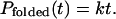
By using a single exponential model for folding (6), the probability that a molecule has folded by time t is expected to be

[1]

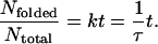
where k is the folding rate. For an ensemble of N_total independent folding simulations, the folding probability P_folded(t) corresponds to N_folded/N_total, with N_folded marking the number of simulations that have reached the folded state by time t. In the limit of t ≪ 1/k, this probability can be approximated as

[2]

Accordingly, the folding time constant can be estimated from the population growth of the folded state as follows (5, 6):

[3]

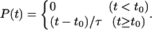
To use this method, a quantitative definition of the folded state is required. In this work, both secondary and tertiary structure components were considered. Namely, we defined a conformation as fully folded when it had native-like secondary structure elements (a β-turn on residues 2–7 and an α-helix on residues 13–20) and an α-carbon root-mean-squared deviation (RMSD_Cα) <3.1 Å from the NMR structure (9, 10). This RMSD_Cα is one standard deviation above the average value of an ensemble of native conformations, which were generated from an independent set of simulations starting from the experimental native conformations (5, 6). A total of 10,000 native conformations were sampled in 1-μs simulation time from 100 independent trajectories (10 ns each) with all simulation protocols identical to the simulations that started unfolded. The population distribution of RMSD_Cα shows a bimodal pattern resulting from equilibration between folded and unfolded states. The average and standard deviation in the folded state were determined by fitting this distribution with two Gaussian curves (see the supporting information, which is published on the PNAS web site).

BBA5 Folding Trajectories in Explicit Solvent

With the definitions outlined above, 13 complete folding events were observed. Fig. 1 shows the population growth of the folded state. It is interesting to see that there is a lag phase before the first folding event. This arises from the fact that the simulations were started from a somewhat extended structure to avoid biasing the resulting folding dynamics. This choice of starting condition allows one to generate a more diverse ensemble of folding events but at the cost of additional molecular dynamics simulation for equilibration to the unfolded state. This equilibration is manifested in the ≈10 ns of simulation required before any folding events occur. To account for this lag phase, fitting for this curve included two parameters: the folding time constant τ and the lag time t₀ with a basis function

[4]

From the TIP3P simulation data, the estimated folding time constant is found to be 4.5 ± 0.4 μs. However, if one corrects for the anomalous viscosity of TIP3P water (18), one gets a time-constant prediction of 7.5 ± 0.7 μs. Both values are in good agreement with the experimental value of 7.5 ± 3.5 μs and the implicit solvation simulation result of 3–13 μs (6). The lag time from the fit is 9.4 ± 0.5 ns. The primary uncertainty in the computed rate does not come from the statistical uncertainty in the fit presented above, but from the systematic error involved with the sensitivity to the folding criteria (6): varying the RMSD_Cα cutoff by ± 0.5 Å results in the folding time constant of 4.5 ± 2.5 μs (before viscosity correction) with 8–10 ns of lag time.

Fig. 1.

Population growth of folded conformation (dotted trace). A linear fitting line for the rate estimation is also presented (solid trace). Vertical gray bars represent SE (one SD) in the population estimation.

In Fig. 2A, snapshots of a folding trajectory leading to the lowest value of RMSD_Cα are presented. One can see that the final folded structure is very similar to the experimental native conformation shown in Fig. 2B. To verify the stability of the folded state thus reached, we have calculated a dwell-time ratio (R_dw) defined as follows:

[5]

This ratio will be close to 1 if the folded conformation obtained from the trajectory is stable within the potential adopted in this work. If the conformation satisfying the folding criteria is not stable, however, it will leave the state in a short amount of time, and the ratio will be close to zero. For the folding trajectories, the average dwell-time ratio was 59%. The average value obtained with the native ensemble was 58%, displaying an exact match within the error of the comparison. Because BBA5 is small, not as stable as large proteins, and quite flexible, one would expect that the dwell-time ratio would be <100%. The flexibility in the native ensemble is observed to be mainly induced by temporary breaks either in tertiary contacts between the helical part and the β-turn of the protein or in the hydrogen bond bridges in the β-turn.

Fig. 2.

(A) Snapshots of a folding trajectory ending to lowest RMSD_Cα. For simplicity, only the backbone and selected hydrophobic side chains (V3, F8, L14, L17, and L18) are shown. The turn (residues 2–7) and the helical (residues 12–20) regions are represented in blue and red, respectively. Three solvent molecules trapped in a hydrophobic pocket are shown in space-fill representation. Numbers in parentheses are RMSD_Cα values. (B) Comparison of the folded structure from the simulations (Left) with the NMR structure (Right). For the simulation structure, conformations with the lowest RMSD_Cα were taken from each of the 13 folding trajectories and aligned to minimize the deviation. The shown structure is a backbone trace of the Cartesian average of all 13 conformations. The same averaging scheme was used for the NMR structure.

Examining the Role of Explicit Water in Hydrophobic Collapse

To examine the role of water in more detail, the first step is to choose particular degrees of freedom, which will yield insight into the folding mechanism. In particular, one should choose degrees of freedom that describe the degree of folding present, the nature of the hydrophobic core, and the nature of the water surrounding the core. Toward this goal, we have inspected the deviation from the native structure (RMSD_Cα), the hydrophobic core size (core radius gyration, R_g), and the solvent density (ρ_solv) along folding trajectories. We define the hydrophobic core to be the side chains of Val-3, Phe-8, Leu-14, Leu-17, and Leu-18. The solvent density was calculated by building cubic grids with 0.25-Å side length, and all grids within van der Waals interaction distance (sum of the core atom and water van der Waals radii) from each of the core atoms were selected after excluding the region occupied by the protein molecule. The number of water molecules in these selected grids were counted and then divided by the volume of the grids available to water molecules.

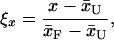
To facilitate direct comparisons, the three metrics described above were reduced to

[6]

where x̄_U and x̄_F represent averages of x from the unfolded and the native ensembles, respectively (with x: R_g, ρ_solv, RMSD_Cα). To obtain statistically meaningful data, all 13 folding trajectories were aligned such that the first sign of folding in each trajectory (i.e., RMSD_Cα ≤ 3.1 Å with correct secondary structure) is shifted to the time t′ = 0, and the values for ξ were averaged over the 13 trajectories at each aligned time point, resulting in the time-dependent reduced variables 〈ξ(t′)〉, which are plotted in Fig. 3.

Fig. 3.

Changes in reduced folding metrics versus shifted time t′: solvent density (black), core radius of gyration (red), and RMSD_Cα (blue). Folding sets in at zero shifted time in each trajectory. For visual clarity, the solvent density was smoothed by taking bins of five adjacent data points. For the reductions, (x̄_U, x̄_F) were obtained from the unfolded and native ensembles, with values of (0.86, 0.73) for the solvent density, (10.4, 6.3) for the core radius of gyration, and (6.6, 3.1) for RMSD_Cα.

The most striking feature we observe is the coincidence between the three metrics: the variations of R_g (degree of collapse) and ρ_solv (degree of solvation/de-wetting) coincide with the variation of RMSD_Cα (degree of folding). Namely, solvent density around the core decreases concurrently with core collapse in this protein, which we will refer to as the “concurrent mechanism” of hydrophobic collapse. Here, we stress that the trajectories were aligned only with the folding criteria (RMSD_Cα and secondary structure elements), and the coincidence of R_g and ρ_solv is not a trivial result of this alignment.

How does this result compare to previous hypotheses regarding the role of water in folding? Recently, ten Wolde and Chandler (1) proposed that evaporation of water in the vicinity of hydrophobic polymer chains may provide the driving force for collapse in folding. They found that the rate-limiting step in the collapse of a hydrophobic polymer is the collective emptying of space around the nucleating sites (“de-wetting mechanism”) with a large vapor bubble forming around the core. After close inspections on our folding trajectories, however, we could not observe such bubbles in our simulations (data not shown).

In some trajectories, however, we find water molecules within a small pocket formed by core residues during the course of folding. In Fig. 2 A, for example, three solvent molecules are found in a pocket formed by core residues after hydrophobic collapse and shortly before the tight packing of the core (19.2 ns), which are then squeezed out as the trajectory reaches a folded conformation (24.4 ns). Qualitatively, this is in agreement with a thermodynamics study by Sheinerman and Brooks (19) and the minimalist Go-model folding simulations of Cheung et al. (2), both of which suggest the expulsion of water molecules in the folding process (“expulsion mechanism”). If hydrophobic collapse always occurs by means of this mechanism, we can expect the solvent density around a hydrophobic group to be equivalent to or higher than the bulk density during the collapse process, reflecting the squeezing-out of water molecules.

The de-wetting and expulsion mechanisms described above differ from one another in the following way. In the de-wetting mechanism, water will avoid proximity to the partially formed core, and this vacuum-surrounded primitive core will spontaneously collapse to stabilize the system by reducing the solvent-accessible surface area of core residues: ξ_ρ would thus decrease first (de-wetting), followed by a change in ξ_Rg (collapse). On the other hand, in the expulsion mechanism, core compaction will precede water expulsion: ξ_Rg would decrease to its native-like value first (potentially with an increase in water density, because of the squeezing of water molecules out of the core), followed by transition to a native-like ξ_ρ.

It is intriguing to consider that the concurrent mechanism observed in our simulations may be generally applicable to the hydrophobic collapse and folding of small proteins. It seems likely that the cores of small proteins (e.g., <50 aa) would be too small to induce the de-wetting effect mentioned above (1). Also, this small core size may limit the relevance of expulsive-like mechanisms seen in Go models (2). Moreover, the very specific nature of solvent separated Go-model native contacts may enhance the likelihood of the expulsion mechanism over what one would see in simulations with more physically based force fields. It will be interesting to see how these three mechanisms interplay in larger proteins whose cores are large enough for the de-wetting and squeezing effects to play more significant roles.

Are Water Degrees-of-Freedom Coupled to the Transition State?

What defines the transition state for folding? Is the transition state completely defined by the protein conformation coordinates or does the particular geometry of water play a role as well? To test whether the particular arrangement of water molecules is important in determining the folding pathway, P_fold simulations were performed. Details of P_fold calculations can be found elsewhere (20, 21). Briefly, 25 configurations were sampled on folding trajectories with their RMSD_Cα values ranging from 1.7–7.5 Å. For each configuration, >100 independent simulations were performed with randomized velocity vectors. Here, P_fold of a given conformation is the probability that it folds within a 5-ns simulation time. For a two-state transition, conformations characterized by P_fold ≈ 0.5 belong to the transition state ensemble and in general, P_fold naturally serves to order conformations along their ideal reaction coordinate (20, 21).

To test whether water coordinates play a role in defining the transition state ensemble, the original water molecules were removed and the conformations used for P_fold simulations were resolvated. The resulting systems were then reequilibrated with 100 ps of molecular dynamics with the protein molecules frozen to the starting conformations, and the newly randomized water conformations were used as the starting systems in a second independent set of P_fold simulations. Differences in P_fold values between this starting ensemble and the original P_fold ensemble would thus indicate changes in the location of the new configuration along the folding pathway, which would in turn confirm that water plays a significant role in defining the transition state ensemble. Fig. 4A shows the relationship between P_fold values from the original and new solvation configuration. It is clear that P_fold values for different solvent configurations are in excellent agreement within the error of our calculations.

Fig. 4.

(A) Correlation of P_fold values with different solvent configurations in the explicit solvation model. Error bars represent one SD for each of the probability predictions. (B) Correlation of P_fold values from implicit and explicit solvation models.

Thus, in our simulations, the protein-folding pathway is determined solely by the protein conformation and not by the surrounding water configurations. This finding can be understood in terms of the difference in time scales of protein and water dynamics. Because the relaxation time for water dynamics is short compared with the protein dynamics time scale, any configuration of water will rerandomize faster than the time scale of the protein-folding transition. This result suggests that it is possible for an implicit solvation model to reproduce explicit solvation results, given that water equilibration appears to be fast relative to that of protein conformational rearrangement. Moreover, this result also suggests that one need not include water degrees-of-freedom explicitly in the interpretation of experimental analyses of the transition state, such as Φ-value analysis (22).

Comparison to Implicit Solvation Models

The de-wetting effect around the hydrophobic group is a liquid–vapor phase equilibrium process, which is not currently described accurately with commonly used implicit solvation models based on estimates of exposed surface area (1). Accordingly, it is natural to ask whether the folding mechanism with such a model will be significantly different from explicit solvent simulation.

For the folding of BBA5 in TIP3P water, we find a diffusion–collision mechanism (23), where secondary structural elements first form independently and then collide to form the native structure. This can be observed by inspecting the probabilities of both secondary structure elements. In Fig. 5, we have compared the joint probability of simultaneously finding both helix and turn (P_α,β) to the product of probabilities for finding helix and turn (P_α·P_β) obtained with conformations at every 1 ns. One can clearly see that the relation P_α,β = P_α·P_β holds for all time windows, suggesting independent formations of secondary structure elements. This mechanism is in agreement with the implicit solvation results of Snow et al. (6), which found a diffusion–collision mechanism with similar statistical independence.

Fig. 5.

Joint probability of finding both turn and helix simultaneously (P_α,β) versus the product of probabilities for finding helix and turn (P_α·P_β) from explicit (A) and implicit (B) solvation simulations (6), showing the statistical independence of secondary structure formation.

To further compare the folding pathways in explicit and implicit solvation models, additional implicit solvation P_fold simulations were performed on the aforementioned 25 configurations by using the Generalized Born/Surface Area continuum solvation model (24) within the tinker package (25) modified for Folding@Home. Other than the solvation model, identical simulation protocols (including the protein force field) were applied as in the explicit solvation simulations to prevent any false discrepancy. If the P_fold values for a given conformation obtained from two different models agree, then the role of that conformation along the folding pathway is similar in both models. For example, if P_fold of a conformation is close to one-half in both cases, then the conformation belongs to the transition state ensemble in both models (20, 21). Thus, the comparison of P_fold values can give a quantitative and statistical comparison between the folding pathways obtained from different models.

Fig. 4B shows the correlations of P_fold values obtained from the two models. Even though there are some notable discrepancies, the two models are in qualitative agreement. This result is in accordance with the findings that the folding rates from both models are similar (4.5 μs versus 6 μs) and that the folding mechanism is qualitatively the same (diffusion–collision) within both models. However, the differences (particularly at low P_fold values for implicit solvation) suggest that explicit solvation models can lead to potentially important differences when compared with implicit solvation, especially when characterizing the transition state.

The lack of a perfect correlation in implicit and explicit solvation models suggests that there are discernable, statistically significant differences in the trajectories created by these models. In Fig. 4, we can see that the P_fold values from the implicit solvation are lower than those from the explicit solvation. After extensive simulations with all 13 folding trajectories, we find that P_fold from the implicit model is consistently lower. Accordingly, we can infer that the transition state (a conformation with P_fold ≈ 0.5) in the implicit model is closer to the folded state than that found in the explicit model. Although a direct comparison of the transition state structures from the two models is rather difficult because of the heterogeneous nature of the folding pathways of this protein, this consistency implies a systematic structural difference between the two models. We speculate that this difference arises from the central gap between the models: the nonadditive and discrete nature of water depicted only in the explicit model. In the implicit model, the system is destabilized by an energy proportional to the solvent accessible surface area (24). In the explicit model of solvation, however, the destabilization is not necessarily proportional to this area if the solvent molecules can cooperatively avoid the vicinity of the hydrophobic groups. This difference leads to an exaggeration of the destabilization energy from the solvent–solute contact in the implicit model. Because the solvent density is lower around/after folding events as shown in Fig. 3, this exaggeration will be larger for the folded state than for the unfolded state. As a consequence, the folded state will be relatively less stable in the implicit model, dragging the transition state toward it by means of the Hammond effect (22).

Our results also suggest that the P_fold method is sensitive enough to detect differences in simulation models or force fields. For example, simulations with electrostatic cutoffs (8) demonstrate nonnegligible differences in P_fold values when compared with reaction field (see the supporting information, which is published on the PNAS web site). We propose that further P_fold analysis can play an important role in studying folding mechanism because this method requires a relatively small amount of CPU time, is trivial to parallelize, and is therefore well suited to grid-based simulation.

Conclusions

We have examined two common, yet radically different models for solvent in molecular simulation, comparing an explicit versus an implicit representation of the solvation. Both models agree well with experimental results on kinetics (rates) as well as in the rough, overall mechanism [diffusion–collision (23)]. Although there is a sign that water is trapped in the core of the protein in the transition state ensemble, it does not play a specific role in the folding dynamics, and only the protein structure is relevant in defining the transition state. In addition, despite the agreement in folding rate and general mechanism, we do find differences in the nature of the transition state ensembles for the two solvation models when more sensitive probes are used. This finding indicates that new experiments are needed to arbitrate between these differences. Indeed, such experiments could open the door to an even greater predictive power for simulations as well as a more detailed understanding of the mechanism of protein folding.

Other simulations have also found discrepancies between explicit and implicit models. For example, Zhou and Berne (26) found that the free energy landscape of a β-hairpin was quite different in the two models. They ascribed this discrepancy to the erroneous strong salt bridges between charged residues in the implicit model. Also, Nymeyer and Garcia (27) reported a profound difference between the models for two α-helical proteins, with the explicit solvation showing good agreement with the experiment. Even though such drastic differences are not observed in our simulations of BBA5, our results are in qualitative agreement with these findings, given that the observed shift in the transition state location in the implicit model must be accompanied by a change in the free energy landscape.

Therefore, it will be interesting to see whether an even more pronounced difference between explicit and implicit solvation models will be found in the simulated folding of other proteins. In this respect, we suggest that direct comparisons of folding simulations from both models will be important both in understanding the protein folding and drawing insights into solvation effects during that process. The ability to conduct such a comparison on other proteins (5) will likely be of great help in deriving a more general framework in which we consider the role of water in the folding mechanism. Through these direct comparisons, the elucidation of the behavior and importance of water near the folding peptide, in terms of both bulk and discrete aqueous properties, may soon be accomplished.

References

- 1.ten Wolde, P. R. & Chandler, D. (2002) Proc. Natl. Acad. Sci. USA 99, 6539-6543. [DOI] [PMC free article] [PubMed] [Google Scholar]
- 2.Cheung, M. S., Garcia, A. E. & Onuchic, J. N. (2002) Proc. Natl. Acad. Sci. USA 99, 685-690. [DOI] [PMC free article] [PubMed] [Google Scholar]
- 3.Teeter, M. M. (1991) Annu. Rev. Biophys. Biophys. Chem. 20, 577-600. [DOI] [PubMed] [Google Scholar]
- 4.Duan, Y. & Kollman, P. A. (1998) Science 282, 740-744. [DOI] [PubMed] [Google Scholar]
- 5.Pande, V. S., Baker, I., Chapman, J., Elmer, S. P., Khaliq, S., Larson, S. M., Rhee, Y. M., Shirts, M. R., Snow, C. D., Sorin, E. J. & Zagrovic, B. (2003) Biopolymers 68, 91-109. [DOI] [PubMed] [Google Scholar]
- 6.Snow, C. D., Nguyen, N., Pande, V. S. & Gruebele, M. (2002) Nature 420, 102-106. [DOI] [PubMed] [Google Scholar]
- 7.Shirts, M. & Pande, V. S. (2000) Science 290, 1903-1904. [DOI] [PubMed] [Google Scholar]
- 8.Lindahl, E., Hess, B. & van der Spoel, D. (2001) J. Mol. Modell. 7, 306-317. [Google Scholar]
- 9.Struthers, M. D., Cheng, R. P. & Imperiali, B. (1996) Science 271, 342-345. [DOI] [PubMed] [Google Scholar]
- 10.Struthers, M., Ottesen, J. J. & Imperiali, B. (1998) Folding Des. 3, 95-103. [DOI] [PubMed] [Google Scholar]
- 11.Garcia, A. E. & Sanbonmatsu, K. Y. (2002) Proc. Natl. Acad. Sci. USA 99, 2782-2787. [DOI] [PMC free article] [PubMed] [Google Scholar]
- 12.Cornell, W. D., Cieplak, P., Barly, C. I., Gould, I. R., Merz, K. M., Ferguson, D. M., Spellmeyer, D. C., Fox, T., Caldwell, J. W. & Kollman, P. A. (1995) J. Am. Chem. Soc. 117, 5179-5197. [Google Scholar]
- 13.Jorgensen, W. L., Chandrasekhar, J., Madura, J. D., Impey, R. W. & Klein, M. L. (1983) J. Chem. Phys. 79, 926-935. [Google Scholar]
- 14.Zagrovic, B., Sorin, E. J. & Pande, V. (2001) J. Mol. Biol. 313, 151-169. [DOI] [PubMed] [Google Scholar]
- 15.Berendsen, H. J. C., Postma, J. P. M., van Gunsteren, W. F., Dinola, A. & Haak, J. R. (1984) J. Chem. Phys. 81, 3684-3690. [Google Scholar]
- 16.Neumann, M. & Steinhauser, O. (1980) Mol. Phys. 39, 437-454. [Google Scholar]
- 17.Hess, B., Bekker, H., Berendsen, H. J. C. & Fraaije, J. G. E. M. (1997) J. Comput. Chem. 18, 1463-1472. [Google Scholar]
- 18.Shen, M. Y. & Freed, K. F. (2002) Biophys. J. 82, 1791-1808. [DOI] [PMC free article] [PubMed] [Google Scholar]
- 19.Sheinerman, F. B. & Brooks, C. L. (1998) J. Mol. Biol. 278, 439-456. [DOI] [PubMed] [Google Scholar]
- 20.Du, R., Pande, V. S., Grosberg, A. Y., Tanaka, T. & Shakhnovich, E. S. (1998) J. Chem. Phys. 108, 334-350. [Google Scholar]
- 21.Pande, V. S. & Rokhsar, D. S. (1999) Proc. Natl. Acad. Sci. USA 96, 9062-9067. [DOI] [PMC free article] [PubMed] [Google Scholar]
- 22.Fersht, A. R. (1998) Structure and Mechanism in Protein Science (Freeman, New York).
- 23.Karplus, M. & Weaver, D. L. (1994) Protein Sci. 3, 650-668. [DOI] [PMC free article] [PubMed] [Google Scholar]
- 24.Qiu, D., Shenkin, P. S., Hollinger, F. P. & Still, W. C. (1997) J. Phys. Chem. A 101, 3005-3014. [Google Scholar]
- 25.Ponder, J. W. (2000) tinker, Software Tools for Molecular Design (Department of Biochemistry and Molecular Biophysics, Washington Univ., St. Louis), Version 3.8.
- 26.Zhou, R. & Berne, B. J. (2002) Proc. Natl. Acad. Sci. USA 99, 12777-12782. [DOI] [PMC free article] [PubMed] [Google Scholar]
- 27.Nymeyer, H. & Garcia, A. E. (2003) Proc. Natl. Acad. Sci. USA 100, 13934-13939. [DOI] [PMC free article] [PubMed] [Google Scholar]
Associated Data
This section collects any data citations, data availability statements, or supplementary materials included in this article.