

Abstract
Hearing instrument design focuses on the amplification of speech to reduce the negative effects of hearing loss. Many amateur and professional musicians, along with music enthusiasts, also require their hearing instruments to perform well when listening to the frequent, high amplitude peaks of live music. One limitation, in most current digital hearing instruments with 16-bit analog-to-digital (A/D) converters, is that the compressor before the A/D conversion is limited to 95 dB (SPL) or less at the input. This is more than adequate for the dynamic range of speech; however, this does not accommodate the amplitude peaks present in live music. The hearing instrument input compression system can be adjusted to accommodate for the amplitudes present in music that would otherwise be compressed before the A/D converter in the hearing instrument. The methodology behind this technological approach will be presented along with measurements to demonstrate its effectiveness.
Keywords: hearing aids, hearing instruments, live music, musicians and hearing loss A/D conversion peak sound pressure level of music
Introduction
Hearing instruments are designed and have been shown to reduce the negative effects of hearing loss (Chisolm et al., 2007; National Council on the Aging [NCOA], 1999). Chisolm et al. (2007) describe hearing instrument use as being a relatively noninvasive, low-risk option for hearing impaired people with many potential benefits. They go on to describe hearing instruments as the only easily accessible treatment for hearing loss, which improves the health-related quality of life in adults by reducing the psychological, social, and emotional effects of sensorineural hearing loss. To address these quality of life issues, hearing instruments are designed to amplify speech signals well, and this is an important key driver behind their development. There is a wide area of research designed to define the characteristics of speech and to subsequently develop amplification schemes in terms of audibility and comfort (American National Standards Institute, 1997; Byrne et al., 1994; Keidser, Dillon, Flax, Ching, & Brewer, 2011; Moore, Glasberg, & Stone, 2010; Scollie et al., 2005). There are, however, hearing instrument users and potential users who require their hearing instruments to amplify live music well, especially with regard to the dynamic characteristics of live music (Killion, 2009; Revit, 2009). These individuals may be professional or amateur musicians or even enthusiastic concert goers. Music, for some individuals, can be considered to be a necessity to enhance their quality of life and at least their feelings of well-being (Levitin, 2006; Menon & Levitin, 2005; Zatorre, 2005). The following article will examine some key considerations in adapting speech-based amplification schemes to meet the needs of hearing instrument users who listen to music. This will include a discussion of the dynamic characteristics of speech and music, along with a discussion of some limitations of signal processing that arise during the conversion of music from the analog to the digital domains.
The Dynamic Characteristics of Speech and Music
Why do hearing instruments typically fail when it comes to reproducing the dynamics of live music? Speech has a well-defined relationship between loudness (the psychological impression of the intensity of a sound) and intensity (the physical quantity relating to the magnitude or amount of sound). For music, this relationship is highly variable and greatly depends on the musical instrument being played (Chasin, 2006a; Fabiani & Friberg, 2011). Speech has many acoustic differences to music regardless of genre, as has been described previously in the literature (Chasin, 2003; Chasin & Russo, 2004). The dynamic characteristics of music create a challenge to the current generation of digital hearing instruments. Many multimemory digital hearing instruments that are available today have music programs. But little is different from other standard speech-specific programs and so the musician cannot experience a natural perception of the dynamics of live music (Chasin, 2003; Zakis & Fulton, 2009).
While clinicians have frequently relied on software fine-tuning to improve the sound quality of music reproduction in digital hearing instruments, the result falls short of what is required because there are many limiting factors that are inherent to the device itself (Chasin, 2010). Such factors might include the quality of miniature transducers, the bandwidth or frequency response of the device, and the dynamic range available in the device. In the past, the transducers used in hearing instruments were frequently blamed for poor fidelity for music. However, this has been shown repeatedly not to be the case (Killion, 1988) and the technology has continued to improve. Extended bandwidth in hearing instruments has also assisted in addressing the mismatch between the frequency response of a hearing instrument (now reported up to 10000Hz) and the frequencies represented in live music (up to 20000Hz). Where sensorineural hearing loss is present, the benefit of extended high frequencies in the hearing instrument will depend on the residual hearing of the user and, in many cases, this will be significantly limited (Ricketts, Dittberner, & Johnson, 2008). Dynamic range, on the other hand, is the factor inherent to hearing instruments with potential for improvement. Although hearing instrument transducers can easily handle the demands of the dynamic range in music, typically these capabilities are not utilized.
One key difference between speech and music is the difference in intensity. Soft speech is generally considered as having a long-term RMS level of 50 dB SPL, conversational speech of 65 dB SPL, and loud speech of 80 dB SPL.1 These input classifications are used to show the amplification response typically seen when measured with a commercially available probe-microphone real ear measurement system, or when simulated by a hearing instrument manufacturer’s software. While there are many different individual variations in the levels of speech, even shouted male speech does not usually exceed 89 dB SPL (Olsen, 1998). Music, on the other hand, is quite different and can easily reach 105 dB (A) and can have peaks of 120 dB (A) or even higher (Killion, 2009; Pawlaczyk-Luszczynska, Dudarewicz, Zamoijska, & Sliwinska-Kowalska, 2010). For example, Killion (2009) measured the peaks of a symphony orchestra in a concert hall at 114 to 116 dB (C), while Flugrath (1969) measured amplified rock music with levels of 114 dB (A). It must be noted that these peaks, especially for orchestral music, are very short in duration and are typically higher than the exposure levels that instrumentalists are subjected to on a long-term basis (Behar, Wong, & Kunov, 2006; MacDonald, Behar, Wong, & Kunov, 2008; Phillips & Mace, 2008; Poissant, Freyman, MacDonald, & Nunes, 2012; Royster, Royster, & Killion, 1991). Amplified rock music, however, can typically have a long-term average level that is higher than that for orchestral music (Clark, 1991).
Typically, a digital hearing instrument compresses the peaks of the signal once they reach 95 dB SPL before the A/D conversion. This is based on the 16-bit analog-to-digital A/D conversion architecture that is employed by most of the hearing instruments currently in use (Agnew, 2002; Edwards, 2007; Hamacher et al., 2005). A compression threshold of 95 dB before the A/D converter is more than adequate even for loud speech, even when the level is measured close to the speaker’s lips. French and Steinberg (1947) found levels of 90 dB SPL, 5.1 cm (2 in.) from the speaker’s lips. Average overall levels are lower as was previously mentioned but this can vary depending on the measurement technique (Byrne, 1977; Cornelisse, Gagné, & Seewald, 1991; Dunn & White, 1940; French & Steinberg, 1947; Ladefoged & McKinney, 1963; Olsen; 1998) For the peaks of live music, this compression threshold of 95dB at the input is too low and the music can sound compressed, unnatural, and even slightly distorted. Compression is used widely in the recording industry to make music sound “louder” and also to make it easier for data reduction for storage on portable devices but is not generally preferred by normal hearing listeners when they are given the choice (Croghan, Arehart, & Kates, 2012). So could the use of low compression thresholds before the A/D converter in hearing instruments be thought of being analogous to the experience of normal hearing individuals when listening to low bit rate encoded music files? This question could be investigated in future studies.
There is nothing that can be done via the hearing instrument software to correct or reduce the effects of this low input compression threshold on the signal. The resulting perceptual distortions are especially a drawback for musicians in ensembles, who may be trying to hear their fellow musicians to play correctly. We will discuss a digital signal processing methodology that can adapt the speech-specific compression limiting at the input to the A/D converter to a music-specific configuration, along with measurements to demonstrate its effectiveness.
A/D Conversion to Accommodate the Dynamics of Live Music
The Fundamentals of A/D Conversion
A/D conversion is part of the front end of the digital hearing instrument. It is comprised of an input source, primarily the hearing instrument microphone, and the A/D converter (Csermak & Armstrong, 1999). A detailed discussion of the process of A/D conversion is beyond the scope of this article; however, a short discussion about it helps to explain the potential solution to this issue. The key element of A/D conversion involved with dynamic range is quantization, which classifies the amplitude information of a signal (Agnew, 2002). To briefly explain quantization, it is necessary to look at some basic definitions. A bit (binary digit) is represented as either a 1 or a 0 and is the smallest possible piece of digital information (Agnew, 2000). The digital word length refers to the number of bits that are used to represent a signal. Therefore, a 16-bit digital word could look like this—1010111001100111. Without focusing on a specific implementation, the quantization step size is generally defined as 2digital word length (Agnew, 2002). Figure 1 shows the dependency of quantization and resolution. The gray curve is part of a sine signal normalized to +/– 0.9 and the black line represent the discrete quantization steps.
Figure 1.
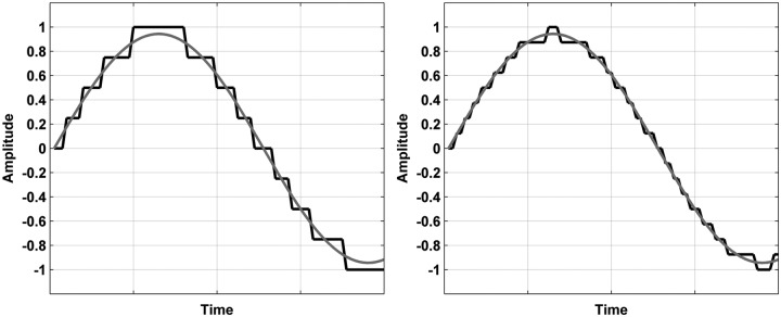
Quantization steps for a portion of a simple waveform
An eight-bit quantization creates 28 or 256 discrete levels to represent the amplitude of a signal as schematically shown on the left side, whereas a 16-bit quantization, shown on the right, will create 216 discrete levels or 65536 levels. The more quantization levels, the more accurate the resolution is for defining the amplitude. Each bit in a digital system represents approximately 6 dB of dynamic range (Ryan & Tewari, 2009). Following this rule, Table 1 shows the relationship between digital word length and dynamic range.
Table 1.
The Relationship Between Digital Word Length and Dynamic Range
| Digital word length | Dynamic range |
|---|---|
| 12 bit * 6 dB | –>72 dB |
| 16 bit * 6 dB | –>96 dB |
| 20 bit * 6 dB | –>120 dB |
| 24 bit * 6 dB | –>144 dB |
| 224 = 16777216 discrete steps |
Most current hearing instruments use 16-bit A/D conversion. However, depending on the hearing instrument design, even if a digital system uses 16-bit A/D conversion, the dynamic range may in fact be limited to only 12 bits, for example, due to other requirements, such as the directional microphone and feedback cancellation processing systems (Agnew, 2000). The result is that to accommodate the peaks of live music, this can only be truly represented by a digital hearing instrument system using A/D conversion of at least 20-bit word lengths resulting in a potential dynamic range of 120 dB.
In addition to the representation of the dynamic range of a signal when converting a signal from analog to digital, it is also important to be aware of quantization error (Lyons, 2004). A large number of discrete steps might not offer infinite precision in the representation of the amplitude because of the quantization error. Due to the fact that the quantization process will always be rounded up or rounded down to the nearest level that is available (Agnew, 2000), the result is that there may be a difference between the actual signal and the quantized signal. This error can produce audible noise, which may be masked by the microphone noise in the hearing instrument. An increase in the number of available quantization levels can be made by increasing the digital word length and this will decrease the quantization error (Agnew, 2002). This enables the digital representation of the analog signal to be more accurate; however, it requires an increase in the power supply to the hearing instrument. To preserve battery life, compromises must be made in the design of the digital hearing instrument. The question remains as to what can be done to improve current digital hearing instrument systems that use 16-bit A/D converters.
Overcoming the Current Limitations of Dynamic Range
Hearing instrument integrated circuits need to be efficient with regard to battery drain and so adjusting the digital word length to accommodate speech while minimizing battery drain is very important. This is one of the main reasons why 20- or even 24-bit A/D conversion is not widely seen in hearing instruments that are currently available today (Kates, 2008). This may, however, change in the future as technology changes. Until then, is there anything that can be done within the hearing instrument, before input compression, to be able to handle the loud peaks of music with 16-bit digital architecture? The answer lies in using a 16-bit A/D converter but shifting the maximum input level where the hearing instrument works more linearly, so that the AGCinput (automatic gain control) does not start to compress until the level from the microphone exceeds approximately 110 dB SPL (Chasin, 2003). This basic idea of modifying the AGCinput was implemented, in a commercially available hearing instrument, by Bernafon AG in 2010. The result is that most, if not all, of the peaks of loud live music are not compressed before the A/D converter without significantly increasing the battery drain, which has been verified by power consumption investigations. In Figure 2, it is possible to see schematically the difference between the shifted (black wave up to 110 dB SPL) and the reference processing (gray wave up to 96 dB SPL) at the front end. Assuming that the gray wave has a sound pressure level of 96 dB SPL, the gray arrow in the AGCinput controller block indicates the cutoff. Input signals with a higher level will not be converted into the digital domain and processed any further. The black wave represents a signal with the characteristics of live music as described above. The black arrow is now changing the AGCinput by shifting the dynamic range toward a higher level by using a delta, “Δ.” However, the range between the min and max value of the amplitude stays the same [–1:1-1/2^(word length-1)] and is not extended like the best case solution with a 20-bit system. After the A/D conversion, this “Δ” will be compensated for elsewhere within the signal processing path of the hearing instrument.
Figure 2.
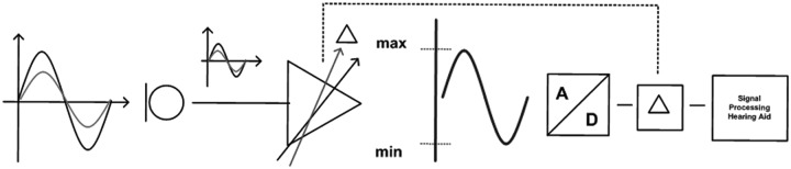
A basic block diagram illustrating the signal path of the A/D conversation
Another way to look at this idea is illustrated in Figure 3, where the behavior of the AGC is shown in an in/output diagram. In the reference situation (black line) the threshold of the AGCinput cuts in at 95 dB SPL, whereas the gray line shows the level-shifted condition that has its threshold at 110 dB SPL because of the implemented attenuation of −15 dB in the AGCinput. This will subsequently be referred to as the “level-shift.”
Figure 3.
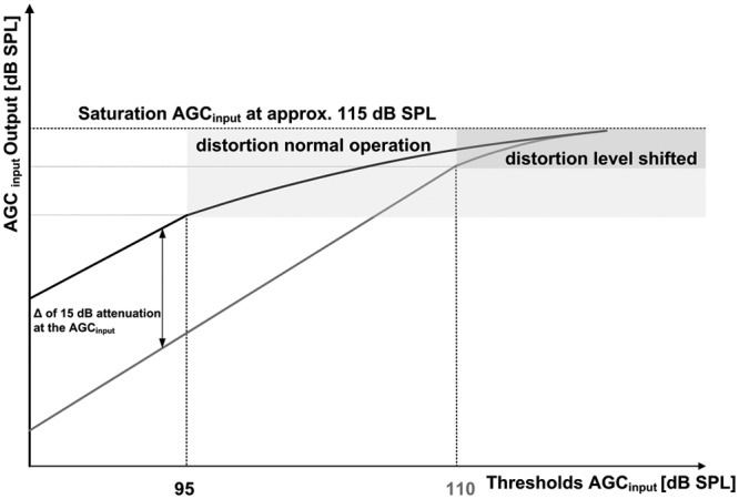
Effect of the AGC input/output behavior for a reference (black line) compared to the level-shifted condition (gray line)
It is very important to emphasize that the level-shift is occurring in the front end, before the amplification within the hearing instrument. The maximum power output (MPO) is therefore not changed. The peaks of music are not increasing the output levels. Short-duration intense sounds in excess of 115 dB SPL create a risk of permanent threshold shift (PTS), as Hunter, Ries, Schlauch, Levine, and Ward (1999) discussed in their study on acoustic reflex testing. The MPO is always set based on the real or calculated uncomfortable loudness levels (UCL) within the hearing instrument to avoid any potential issues of PTS or even temporary threshold shift (TTS) for the hearing instrument user. The usual care should be taken when setting the MPO regardless of input.
Acoustical Measurements With a Modified Input AGC
A series of measurements was conducted to verify the effectiveness of the level-shift within the digital front end of a hearing instrument.
Method, Equipment, and Setup
All measurements were performed with the same setup. A custom programmed LabVIEW 2010 SP1 (National Instruments Corporation, Austin, Texas) based recording tool was used, which gives the opportunity to do real-time input/output measurements. The chassis from a National Instruments (NI) MPXI-1024 with an embedded controller NI PXI-8108 and the analog signal acquisition and generation card NI PXI-4461 were integrated into the setup as shown in Figure 4. The signals were recorded via a Bruel & Kjaer 2cc Coupler 4946 connected to a G.R.A.S. AG 40 microphone with the G.R.A.S. Type 26 A preamplifier and 12 AA power supply. The signals were presented in the free-field via a multichannel power amplifier, RAM Audio T2408, connected to a stand-mounted Bose MA 12 Line Array loud speaker (LS).
Figure 4.
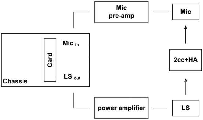
Measurement setup
The hearing instrument was placed on a stand 40 cm away from and pointing toward the middle of the loud speaker. A sound-absorbing curtain covered any reflective surfaces in a 30m2 quiet room. Two different acoustic stimuli were used. The first consisted of sine signals of 1 kHz and 3 kHz, while the second consisted of a mixture of small recorded excerpts of music, 15 to 30 s in duration, representing different styles and genres of music with broad dynamic changes (e.g., choir and orchestra: Elgar The Dream of Gerontius). All signals were normalized to +/– 1 with Adobe Audition 3.0 (Adobe Systems Incorporated, San Jose, California). Recordings were used to control as many variables as possible within the test room and also to ensure the reliability and repeatability of the measurements. An integrated calibration routine ensured that the desired sound level was applied at the calibration point. The hearing instrument used was a commercially available BTE unit, chosen randomly from stock.
Two conditions were compared, first, a reference program with all adaptive features deactivated; and second, the level-shifted program with the modified AGCinput. For comparison reasons, the gain was set to the same linear values via the fitting software with minimal amplification to isolate the front end of the hearing instrument as much as possible (Chasin, 2006b), as can be seen in Figure 5. The amplification was chosen to be rather small to avoid any interaction with the MPO of the hearing instrument. The expansion system was set to the maximum to overcome the possible side effects of the internal and external noise floors. No other special settings were used.
Figure 5.
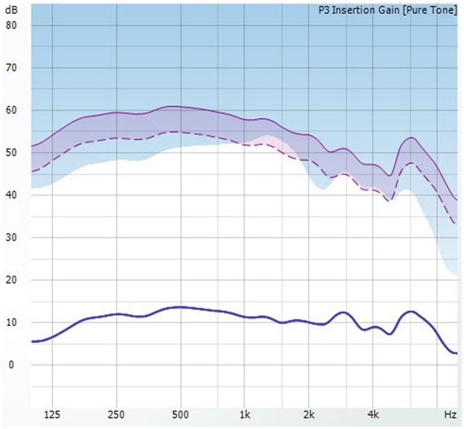
Linear insertion gain simulation of the hearing instrument
Results
An easy way to see the difference between the preamplification of the reference and level-shifted conditions is by looking at an input/output function. In Figure 6, we can see an input/output function for a 1000Hz sine signal with the gain setting shown in Figure 5. The gray line represents the reference program designed for speech with a 95 dB SPL cutoff. After the 95 dB SPL input, the curve begins to level off, indicating that the instrument is compressing this signal. The black line represents the same instrument but with the AGCinput cutoff moved to 110 dB SPL. In this case, the hearing instrument is not compressing the signals within the front end until they reach beyond 110 dB SPL.
Figure 6.

Input/output function with the level-shifting processing on and off for a 1 kHz sine signal
Even when the gain is increased by 4 dB in the hearing instrument, the effect is still clearly seen as shown in Figure 7. To emphasize the functionality, an additional measurement with a 3 kHz sine signal was performed (Figure 8).
Figure 7.

Input/output function with the level-shifting processing on and off for a 1 kHz sine signal—gain increased by 4 dB compared to Figure 6
Figure 8.

Input/output function with the level-shifting processing on and off for a 3 kHz sine signal
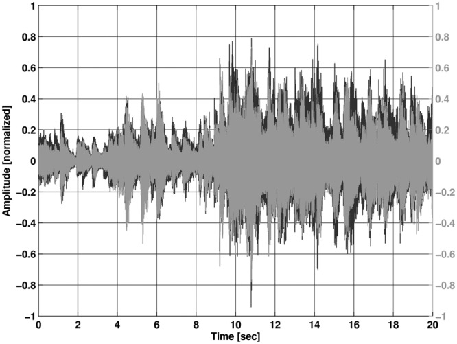
The saturation knee point for the 3 kHz input is shifted toward lower input levels due to characteristics of the microphone resonances. Pure sine wave signals are not so common in music (except electronic music), so it is important to look at the effects that have been seen so far with recordings of music. In the following figures, we see recorded music displayed as waveforms with normalized amplitude on the y-axis and time on the x-axis. The black waveform is always the original signal while the gray represents the signal through the hearing instrument. In Figures 9 and 10, two gray .wav files for a 110 dB SPL peak input are shown that are recordings from a selection of music from the first movement (Vivace) of Beethoven’s Symphony No. 7.
Figure 9.
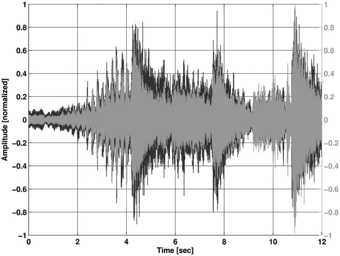
Recording with level-shifted processing; input level 110 dB SPL
Note: The black waveform is the original input file.
Figure 10.
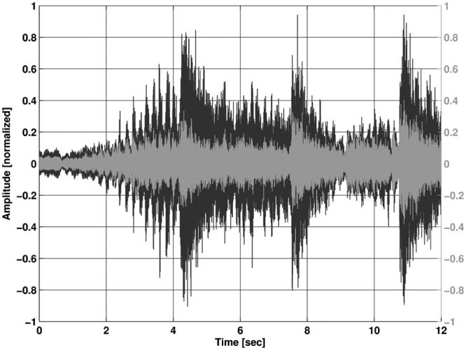
Recording with reference processing; input level 110 dB SPL
Note: The black waveform is the original input file.
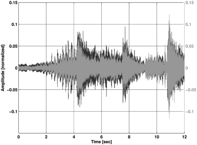
Figures 9 and 10 clearly show the effect of the preserved dynamic range with the level-shifted processing in comparison with the reference signal where compression is applied to the signal at the input. This demonstrates that the natural dynamic characteristics will be converted into the digital domain with the level-shift. It is also of interest to see how the level-shifted processing affects smaller input levels. The following Figures, 11 and 12 show the recordings with the same input signal but with a level of 90 dB SPL.
Figure 11.

Recording with level-shifted processing; input level 90 dB SPL
Note: The black waveform is the original input file.
Figure 12.
Recording with reference processing; input level 90 dB SPL
The black waveform is the original input file.
When the input is reduced, the effect heavily decreases and the reference processing can preserve the same dynamic behavior as the level-shifted processing. The effect has been shown so far by just one piece of orchestral music. To emphasize the effect, the following Figures 13 and 14 show a recording with a 110 dB SPL peak input of a small brass ensemble playing a traditional American Jazz piece, St. James Infirmary. Again, the preservation of the dynamic range is clearly shown in Figure 13 compared to the reference processing in Figure 14.
Figure 13.
Recording with level-shifted processing; input level 110 dB SPL
The black waveform is the original input file.
Figure 14.

Recording with reference processing; input level 110 dB SPL
The black waveform is the original input file.
These measurements were all made with recordings from CD sources (16-bit 44.1 kHz Stereophile and EMI) to ensure the reliability and repeatability of the measurements. It is possible, however, to predict that for live performances with a greater dynamic range the effects of the level-shift would be even greater.
Side Effects From the Level-shift
Are there any negative effects to the level-shift? When making this level-shift, there is one side effect that is generated. By attenuating the AGCinput, all input levels are shifted and special care has to be taken into account for soft inputs. For hearing instrument users who have normal low-frequency hearing, the internal noise of the hearing instrument may be more audible in quiet environments than for a comparable program that is designed for speech without the level-shift. On the other hand, the level of the music (even pianissimo) is likely to be much more intense than the circuit noise, so any perceivable noise will probably be masked (M. Chasin, personal communication, October 19, 2012). To overcome this potential issue, in the level-shifted program, the threshold for the frequency-weighted expansion system was adjusted to compensate for this side effect. Expansion is the opposite of compression; more specifically, less gain is applied to soft sounds (Venema, 2006). Expansion can reduce the internal noise within the hearing aid and additionally will also reduce low-level steady state environmental noise such as that produced by ventilation systems and so forth.
Additional Considerations for Hearing Instrument Music Programs
It is possible to apply the input level-shift to different programs within a multimemory hearing instrument. The settings needed to make this change are, therefore, not global. So it is not necessary to have all end user settings with the level-shift engaged. The result is that a dedicated program can be used within the hearing instrument purely for music. In addition to the level-shift in the front end for higher input levels, is there anything else that can be done to make live music more enjoyable? With regard to a program for live music the following additional factors were considered: bandwidth and amplification, the use of automatic systems, and throughput delay.
Bandwidth and Amplification
It is well known that for normal hearing listeners a wide frequency response contributes to the perceived naturalness of music (Moore & Tan, 2003). Efforts were made to ensure that the frequency response of the hearing instruments using the level-shifts were as wide as possible—up to 10 kHz depending on the style and acoustic coupling method. It must be remembered, however, that hearing impaired listeners may not all prefer an extended high frequency response (Franks, 1982; Punch, 1978). This may be due to the individual’s hearing loss, where individuals with milder hearing losses prefer more high frequency bandwidth (Ricketts et al., 2008). With regard to low-frequency amplification, Franks (1982) concluded that hearing impaired listeners prefer an extended low-frequency response when listening to music. However, due to the use of open fittings, much of the low-frequency amplification of the hearing instrument is reduced while more of the natural low-frequency information passes naturally through the acoustic coupling to the ear. For a further discussion on hearing instrument bandwidth issues and music please see Moore (2012).
In addition to a wider bandwidth, the amount of compression prescribed by the fitting algorithm for the hearing instrument user was reduced in the music program with the level-shift applied. Using offset tables, a more linear response was provided by the fitting software. This is consistent with the studies that suggest different amplification strategies could be applied to music in contrast to speech (Chasin & Russo, 2004; Davies-Venn, Souza, & Fabry, 2007; van Buuren, Festen, & Houtgast, 1996, 1999). The clinician can of course apply the gain and adjust the compression parameters that are desirable for a particular hearing instrument user with the fitting software, so issues such as comfort or other specific requests can be easily accommodated.
Automatic Features
When listening to music, it is important that all automatic features such as noise reduction and adaptive directionality are turned off. This is important to prevent these systems from interpreting the music as noise that may affect the sound quality (Chasin & Russo, 2004; Russo, 2006). When sitting in a concert hall, it is often the case that the people in the seats around the listener make extraneous noise. Perhaps they are explaining what is happening on stage to their neighbor. Or, perhaps they are opening a sweet wrapper, which can be very disruptive, no matter how slowly they do it (Kramer, 2000). Applause can also be very loud and disruptive while wearing hearing instruments in a concert. It is desirable therefore to select a fixed directional microphone setting, if needed, in a live music program, to place the focus on stage and not so much on the activities of the audience members around the listener.
Throughput Delay
A number of studies have investigated the effect of throughput delay on sound quality. This delay refers to the sum of delays inherent in the signal path of the hearing instrument and typically falls below 10 ms (Dillon, Keidser, O’Brien, & Silberstein, 2003). Although studies testing delays in the range of 1 to >10 ms in simulation have demonstrated negative effects on sound quality as judged by normal and impaired hearing listeners (Stone & Moore, 1999, 2002, 2003, 2005; Stone, Moore, Meisenbacker, & Derleth, 2008), these negative effects were not evident when testing in real hearing instruments worn by hearing impaired listeners (Groth & Sondergard, 2004). One study by Zakis, Fulton, and Steele (2012) examined the effect of throughput delay on the sound quality of music in real hearing instruments. In this study, an attempt was made to create a worst case scenario by using open-canal hearing instruments with the gain set such that the likelihood of comb filtering was maximized. Comb filter effects were anticipated when the amplified signal and direct signal paths are combined in the ear canal of the listener. Twelve trained musicians listened to two selected music passages under three delay conditions (1.4, 2, and 3.4 ms) and a no-delay condition. Although differences in sound quality could be described by the musicians for each delay condition, and in some cases strong preferences were recorded for individuals, no significant difference was found between preferences assigned to each delay condition compared to the no-delay condition.
Experience With a Hearing Instrument Utilizing the Input Level-Shift
Dedicated programs for live music, which take account of the additional factors discussed above, are used in current hearing instruments. It is important to determine if subjective improvements can be found when the level-shift in the front end for higher input levels is implemented and used by individuals, who had reported previous poor experience with digital hearing instruments. Hockley et al. (2010) conducted a study which looked at the ratings of sound quality attributes by 9 professional musicians (8 males and 1 female). Four of these musicians were woodwind players (clarinet, saxophone, and flute); 3 played jazz, while the other was a classical musician. Three of the musicians were classical violinists who also played the viola. The final two musicians were both rock (electric) guitarists. These individuals were all current users of analog K-AMP™ custom canal hearing instruments (Killion, 1990, 1993). These individuals had not been able to wear digital hearing instruments due to their reports of unnatural sound quality, which ultimately disrupted the playing and enjoyment of music. The nine musicians were fitted with Micro BTE hearing instruments. Eight wore nonoccluding ear molds, while one used fully occluding earmolds.
The attribute scales used with the participants were based on the work of Gabrielsson, Rosenberg, and Sjögren (1974), Gabrielsson and Sjögren (1979), Gabrielsson, Lindström, and Ove (1991), and Cox and Alexander (1983). The scales consisted of qualitative descriptions of sound quality. Each participant gave a numerical rating toward the attribute that best suited what he or she experienced. Fullness is an example of an attribute that was used, where the perceptual dimension is from “full” to “thin.” Another example of an attribute that was measured is for naturalness, where the perceptual dimension is from “true to the source” to “artificial.” The participants were asked to compare, with the same hearing instruments, a program that applied the level-shift with a standard program that did not.
Overall, for the judgment of fullness, a program with the level-shift was judged to be significantly fuller than for the standard program without the level-shift. Overall fidelity for the level-shifted program was judged to be significantly better than for the standard program. There was no significant difference between the judgments of naturalness between the two programs due to a large variance in the response data; however, a trend was observed. In this small investigation it was concluded that the level-shift contributed to a better rating of sound quality for these musicians.
Summary and Conclusions
Musicians and music enthusiasts have high expectations with regard to their hearing instrument performance for music. These expectations are rarely met. While continuing improvements in miniaturized transducers and bandwidth have helped, an opportunity exists to further improve performance for music by adapting the dynamic range of hearing instruments. This article described the implementation of a solution to accommodate the loud peaks of live music that would otherwise be compressed or even distorted before the A/D converter used in the 16-bit architecture applied in many hearing instruments today. The use of this level-shift preserves the dynamics of live music for musicians and music enthusiasts without affecting the battery life. As digital hearing instrument technology evolves toward 20-bit and even 24-bit architecture to accurately convey at least a 120 dB dynamic range, with less current consumption, then the use a level-shift will be obsolete. The use of a level-shift is the most practical solution for music for the hearing instrument architecture that is most commonly available today. The improvement was evident in the subjective assessment by a group of musicians who had previously rejected digital processing hearing instruments in favor of an analog instrument. As tested by Hockley et al. (2010), the judgments of sound quality revealed that when wearing digital hearing instruments, these musicians preferred a program with the level-shift engaged for live music.
Acknowledgments
The authors thank Stefan Marti, Simon Schüpbach, and Miquel Sans for their technical descriptions of the implementation and Christian Glück for programming the software for the LabVIEW tests. The authors also thank Jennifer Hockley, Barbara Simon, Christophe Lesimple, and an anonymous reviewer for comments on earlier versions of this article.
Scollie et al. (2005) in their discussion of the DSL m[i/o] algorithm have proposed that these values should be changed to the following: Soft speech is 52 dB, Average speech is 60 dB, and Loud speech is 74 dB.
Footnotes
Authors’ Note: The authors are paid employees of Bernafon AG, Berne, Switzerland.
Declaration of Conflicting Interests: The authors declared no potential conflicts of interest with respect to the research, authorship, and/or publication of this article.
Funding: The authors received no financial support for the research, authorship, and/or publication of this article.
References
- Agnew J. (2000). Digital hearing aid terminology made simple: A handy glossary. Hearing Journal, 53(3), 37-43 [Google Scholar]
- Agnew J. (2002). Amplifiers and circuit algorithms for contemporary hearing aids. In Valente M. (Ed.), Hearing aids: Standards, options and limitations (2nd ed., pp. 101-142), New York, NY: Thieme [Google Scholar]
- American National Standards Institute. (1997). ANSI S3.5-1997: Methods for the calculation of the speech intelligibility index. New York, NY: Author [Google Scholar]
- Behar A., Wong W., Kunov H. (2006). Risk of hearing loss in orchestra musicians: Review of the literature. Medical Problems of Performing Artists, 21, 164-168 [Google Scholar]
- Byrne D. (1977). The speech spectrum: Some aspects of its significance for hearing aid selection and evaluation. British Journal of Audiology, 11, 40-46 [DOI] [PubMed] [Google Scholar]
- Byrne D., Dillon H., Tran K., Arlinger S., Wilbraham K., Cox R., Ludvigsen C. (1994). An international comparison of long-term average speech spectra. Journal of the Acoustical Society of America, 96, 2108-2120 [Google Scholar]
- Chasin M. (2003). Music and hearing aids. Hearing Journal, 56(7), 36-41 [Google Scholar]
- Chasin M. (2006a). Hearing aids for musicians. Hearing Review, 13(3), 11-16 [Google Scholar]
- Chasin M. (2006b). Can your hearing aid handle loud music? A quick test will tell you. Hearing Journal, 63(12), 22-24 [Google Scholar]
- Chasin M. (2010). Six ways to improve listening to music through hearing aids. Hearing Journal, 63(9), 27-30 [Google Scholar]
- Chasin M., Russo F. A. (2004). Hearing aids and music. Trends in Amplification, 8(2), 35-47 [DOI] [PMC free article] [PubMed] [Google Scholar]
- Chisolm T. H., Johnson C. E., Danhauer J. L., Portz L. J. P., Abrams H. B., Lesner S., Newman C. W. (2007). A systematic review of health-related quality of life and hearing aids: Final report of the American Academy of Audiology task force on the health-related quality of life benefits of amplification in adults. Journal of the American Academy of Audiology, 18, 151-183 [DOI] [PubMed] [Google Scholar]
- Clark W. W. (1991). Noise exposure from leisure activities: A review. Journal of the Acoustical Society of America, 90, 175-181 [DOI] [PubMed] [Google Scholar]
- Cornelisse L. E., Gagné J.-P., Seewald R. C. (1991). Ear level recordings of the long-term average spectrum of speech. Ear and Hearing, 12(1), 47-54 [DOI] [PubMed] [Google Scholar]
- Cox R. M., Alexander G. C. (1983). Acoustic versus electronic modifications of hearing aid low-frequency output. Ear and Hearing, 4, 190-196 [DOI] [PubMed] [Google Scholar]
- Croghan N. B. H., Arehart K. H., Kates J. M. (2012). Quality and loudness judgements for music subjected to compression limiting. Journal of the Acoustical Society of America, 132, 1177-1188 [DOI] [PubMed] [Google Scholar]
- Csermak B., Armstrong S. (1999). Bits, bytes & chips: Understanding digital hearing instruments. Hearing Review, 6(1), 8-12 [Google Scholar]
- Davies-Venn E., Souza P., Fabry D. (2007). Speech and music quality ratings for linear and nonlinear hearing aid circuitry. Journal of the American Academy of Audiology, 18, 688-699 [DOI] [PubMed] [Google Scholar]
- Dillon H., Keidser G., O’Brien A., Silberstein H. (2003). Sound quality comparisons of advanced hearing aids. Hearing Journal, 56(4), 30-40 [Google Scholar]
- Dunn H. K., White S. D. (1940). Statistical measurements on conversational speech. Journal of the Acoustical Society of America, 11, 278-288 [Google Scholar]
- Edwards B. (2007). The future of hearing aid technology. Trends in Amplification, 11(1), 31-45 [DOI] [PMC free article] [PubMed] [Google Scholar]
- Fabiani M., Friberg A. (2011). Influence of pitch, loudness, and timbre on the perception of musical instruments. Journal of the Acoustical Society of America, 130, EL193-EL199 [DOI] [PubMed] [Google Scholar]
- Flugrath J. M. (1969). Modern-day rock-and-roll music and damage risk criteria. Journal of the Acoustical Society of America, 45, 704-711 [DOI] [PubMed] [Google Scholar]
- Franks R. J. (1982). Judgements of hearing aid processed music. Ear and Hearing, 3(1), 18-23 [DOI] [PubMed] [Google Scholar]
- French N., Steinberg J. (1947). Factors governing the intelligibility of speech sounds. Journal of the Acoustical society of America, 19, 90-119 [Google Scholar]
- Gabrielsson A., Lindström B., Ove T. (1991). Loudspeaker frequency response and perceived sound quality. Journal of the Acoustical Society of America, 90, 707-719 [Google Scholar]
- Gabrielsson A., Rosenberg U., Sjögren H. (1974). Judgements and dimension analyses of perceived sound quality of sound-reproducing systems. Journal of the Acoustical Society of America, 55, 854-861 [DOI] [PubMed] [Google Scholar]
- Gabrielsson A., Sjögren H. (1979). Perceived sound quality of hearing aids. Scandinavian Audiology, 8, 159-169 [DOI] [PubMed] [Google Scholar]
- Groth J., Sondergaard M. B. (2004). Disturbance caused by varying propogation delay in non-occluding hearing aid fittings. International Journal of Audiology, 43, 594-599 [DOI] [PubMed] [Google Scholar]
- Hamacher V., Chalupper J., Eggers J., Fischer E., Kornagel U., Puder H., Rass U. (2005). Signal processing in high-end hearing aids: State of the art, challenges, and future trends. Journal on Applied Signal Processing, 18, 2915-2929 [Google Scholar]
- Hockley N. S., Bahlmann F., Chasin M. (2010). Programming hearing instruments to make live music more enjoyable. Hearing Journal, 63(9), 30-38 [Google Scholar]
- Hunter L. L., Ries D. T., Schlauch R. S., Levine S. C., Ward W. D. (1999). Safety and clinical performance of acoustic reflex tests. Ear and Hearing, 20, 506-514 [DOI] [PubMed] [Google Scholar]
- Kates J. M. (2008). Digital hearing aids. San Diego, CA: Plural [Google Scholar]
- Keidser G., Dillon H., Flax M., Ching T., Brewer S. (2011). The NAL-NL2 prescription procedure. Audiology Research, 1, e24. [DOI] [PMC free article] [PubMed] [Google Scholar]
- Killion M. C. (1988). Technological report: An “acoustically invisible” hearing aid. Hearing Instruments, 39(10). Retrieved from www.etymotic.com [Google Scholar]
- Killion M. C. (1990). A high fidelity hearing aid. Hearing Instruments, 41(8). Retrieved from www.etymotic.com [Google Scholar]
- Killion M. C. (1993). The K-AMP hearing aid: An attempt to present high fidelity for the hearing impaired. In Beilin J., Jensen G. R. (Eds.), Recent developments in hearing instrument technology: 15th Danavox Symposium (pp. 167-229). Copenhagen, Denmark: Stougaard Jensen [Google Scholar]
- Killion M. C. (2009). What special hearing aid properties do performing musicians require? Hearing Review, 16(2), 20-31 [Google Scholar]
- Kramer E. M. (2000, June 2). On the noise from a crumpled candy wrapper. Popular version of paper 4pPa2 presented at the Acoustical Society of America 139th Meeting, Atlanta, GA [Google Scholar]
- Ladefoged P., McKinney N. P. (1963). Loudness, sound pressure and subglottal pressure in speech. Journal of the Acoustical Society of America, 35, 454-460 [Google Scholar]
- Levitin D. J. (2006). This is your brain on music: The science of a human obsession. New York, NY: Dutton/Penguin [Google Scholar]
- Lyons R. G. (2004). Understanding digital signal processing (2nd ed.). Upper Saddle River, NJ: Prentice Hall [Google Scholar]
- MacDonald E. N., Behar A., Wong W., Kunov H. (2008). Noise exposure of opera musicians. Canadian Acoustics, 36(4), 11-16 [Google Scholar]
- Menon V., Levitin D. J. (2005). The rewards of music listening: Response and physiological connectivity of the mesolimbic system. NeuroImage, 28, 175-184 [DOI] [PubMed] [Google Scholar]
- Moore B. C. J. (2012). Effects of bandwidth, compression speed, and gain at high frequencies on preferences for amplified music. Trends in Amplification, 16, 159-172 [DOI] [PMC free article] [PubMed] [Google Scholar]
- Moore B. C. J., Glasberg B. R., Stone M. A. (2010). Development of a new method for deriving initial fittings for hearing aids with multi-channel compression: CAMEQ2-HF. International Journal of Audiology, 49, 216-227 [DOI] [PubMed] [Google Scholar]
- Moore B. C. J., Tan C.-T. (2003). Perceived naturalness of spectrally distorted speech and music. Journal of the Acoustical Society of America, 114, 408-418 [DOI] [PubMed] [Google Scholar]
- National Council on the Aging. (1999). The consequences of untreated hearing loss in older persons. Washington, DC: Author; [PubMed] [Google Scholar]
- Olsen W. A. (1998). Average speech levels and spectra in various speaking/listening conditions: A summary of the Pearson, Bennett, and Fidell (1977) report. American Journal of Audiology, 7, 1-5 [DOI] [PubMed] [Google Scholar]
- Pawlaczyk-Luszynska M., Dudarewicz A., Zamoijska M., Sliwinska-Kowalska M. (2010, June). Evaluation of sound exposure and risk of hearing impairment in orchestral musicians. Paper presented at the 15th International Conference on Noise Control, Ksiaz-Wroclaw, Poland Retrieved from www.earcom.pl [Google Scholar]
- Phillips S. L., Mace S. (2008). Sound level measurements in music practice rooms. Music Performance Research, 2, 36-47 [Google Scholar]
- Poissant S. F., Freyman R. L., MacDonald A. J., Nunes H. A. (2012). Characteristics of noise exposure during solitary trumpet playing: Immediate impact on distortion-product otoacoustic emissions and long-term implications for hearing. Ear and Hearing, 33, 543-553 [DOI] [PubMed] [Google Scholar]
- Punch J. L. (1978). Quality judgements of hearing aid-processed speech and music by normal and otopathologic listeners. Journal of the American Auditory Society, 3, 179-188 [PubMed] [Google Scholar]
- Revit L. J. (2009). What’s so special about music? Hearing Review, 16(2), 12-19 [Google Scholar]
- Ricketts T. A., Dittberner A. B., Johnson E. E. (2008). High-frequency amplification and sound quality in listeners with normal through moderate hearing loss. Journal of Speech, Language and Hearing Research, 51, 160-172 [DOI] [PubMed] [Google Scholar]
- Royster J. D., Royster L. H., Killion M. C. (1991). Sound exposures and hearing thresholds of symphony orchestra musicians. Journal of the Acoustical Society of America, 89, 2793-2803 [DOI] [PubMed] [Google Scholar]
- Russo F. A. (2006). Perceptual considerations in designing and fitting hearing aids for music. Hearing Review, 13(3), 74-78 [Google Scholar]
- Ryan J., Tewari S. A. (2009). A digital signal processor for musicians and audiophiles. Hearing Review, 16(2), 38-41 [Google Scholar]
- Scollie S., Seewald R., Cornelisse L., Moodie S., Bagatto M., Launagaray D., Pumford M. (2005). The desired sensation level multistage input/output algorithm. Trends in Amplification, 9, 159-197 [DOI] [PMC free article] [PubMed] [Google Scholar]
- Stone M. A., Moore B. C. J. (1999). Tolerable hearing aid delays: I. Estimation of limits imposed by the auditory pathway alone using simulated hearing losses. Ear and Hearing, 20, 182-192 [DOI] [PubMed] [Google Scholar]
- Stone M. A., Moore B. C. J. (2002). Tolerable hearing aid delays: II. Estimation of limits imposed during speech production. Ear and Hearing, 23, 325-338 [DOI] [PubMed] [Google Scholar]
- Stone M. A., Moore B. C. J. (2003). Tolerable hearing aid delays: III. Effects on speech production and perception of across-frequency variation in delay. Ear and Hearing, 24, 175-183 [DOI] [PubMed] [Google Scholar]
- Stone M. A., Moore B. C. J. (2005). Tolerable hearing aid delays: IV. Effects on subjective disturbance during speech production by hearing-impaired subjects. Ear and Hearing, 26, 225-235 [DOI] [PubMed] [Google Scholar]
- Stone M. A., Moore B. C. J., Meisenbacker K., Derleth R. P. (2008). Tolerable hearing aid delays: V. Estimation of limits for open canal fittings. Ear and Hearing, 29, 601-617 [DOI] [PubMed] [Google Scholar]
- van Buuren R. A., Festen J. M., Houtgast T. (1996). Peaks in the frequency response of hearing aids: Evaluation of the effects on speech intelligibility and sound quality. Journal of Speech and Hearing Research, 39, 239-250 [DOI] [PubMed] [Google Scholar]
- van Buuren R. A., Festen J. M., Houtgast T. (1999). Compression and expansion of the temporal envelope: Evaluation of speech intelligibility and sound quality. Journal of the Acoustical Society of America, 105, 2903-2913 [DOI] [PubMed] [Google Scholar]
- Venema T. H. (2006). Compression for clinicians (2nd ed.). Clifton Park, NY: Delmar Cengage Learning [Google Scholar]
- Zakis J. A., Fulton B. (2009). How can digital signal processing help musicians? Hearing Review, 16(5),44-48 [Google Scholar]
- Zakis J. A., Fulton B., Steele B. (2012). Preferred delay and phase-frequency response of open-canal hearing aids with music at low insertion gain. International Journal of Audiology, 51, 906-913 [DOI] [PubMed] [Google Scholar]
- Zatorre R. (2005). Music, the food of neuroscience? Nature, 434, 312-315 [DOI] [PubMed] [Google Scholar]