

Abstract
The relative income or income status hypothesis implies that people should be happier when they live among the poor. Findings on neighborhood effects suggest, however, that living in a poorer neighborhood reduces, not enhances, a person’s happiness. Using data from the American National Election Study linked to income data from the U.S. census, the authors find that Americans tend to be happier when they reside in richer neighborhoods (consistent with neighborhood studies) in poorer counties (as predicted by the relative income hypothesis). Thus it appears that individuals in fact are happier when they live among the poor, as long as the poor do not live too close.
This study investigates whether the happiness of Americans is affected by the income of those living nearby. If one’s status relative to one’s neighbors is what matters (e.g., Veblen 1899), then Americans should be happier living among the poor (other things equal), as a few recent studies have found (e.g., Luttmer 2005). Those studies are based, however, on “neighborhoods” that range in size from spatial units averaging about 150,000 residents (Luttmer 2005) to entire U.S. states (Blanchflower and Oswald 2004). In this research we use much smaller geographic units because we want to investigate the effect of the incomes of nearby neighbors on happiness.
In the case of nearby neighbors, there are opposing types of relative status to take into account: neighborhood income compared to own income and neighborhood income compared to average income in the more general region. The first implies lower relative status when a person lives in a high-income neighborhood, whereas the second implies higher status when a person lives in a high-income neighborhood. Moreover, neighborhood amenities, such as well-maintained housing units and safe streets, covary with neighborhood income in the United States. Even though someone personally has lower relative status in a richer neighborhood, those Veblen status effects might be submerged by the effects of the greater prestige and better amenities associated with a richer neighborhood.2
We do not know which effects prevail because no one has examined the effect of local neighborhood income on happiness, net of the effects of own income and regional income.3 That is the aim of this study.
We set the stage by describing the Easterlin paradox, a notable feature of many Western societies that has kindled substantial scholarly interest in income status or relative income effects on happiness (Clark, Frijters, and Shields 2008). Before we examine that paradox, though, it is useful to consider why sociologists might be interested in the study of happiness in the first place, since happiness generally has not been a major concern in the discipline.
WHY SHOULD SOCIOLOGISTS STUDY HAPPINESS?
There is credible evidence that happiness has significant real-life consequences. In a longitudinal study, for example, Koivumaa-Honkanen et al. (2003) found that self-reported happy people are much less likely to commit suicide. In fact, happier people might even have longer life expectancy for reasons unrelated to suicide. One study, based on an analysis of autobiographies that nuns in Milwaukee and Baltimore were required to write when they joined their convents in the 1930s, found a strong association between positive emotional content (e.g., happiness, contentment) in the autobiographies and longevity six decades later (Danner, Snowdon, and Friesen 2001).4 As a result of these and other findings in the social, medical, and neurosciences, scholarly interest in happiness has surged in recent years (Diener et al. 1999; Frey and Stutzer 2002; Kahneman, Diener, and Schwarz 2003; Layard 2005; Gilbert 2006; Klein 2006; Nettle 2006; Veenhoven 2008). This surge is apparent both in economics—where Clark et al. (2008, p. 95) note that “studying the causes and correlates of human happiness has become one of the hot topics in economics over the last decade”—and in psychology, where a new branch called “positive psychology” focuses on making normal life more satisfying rather than on curing mental illness (Csikszentmihalyi 1990; Seligman 2002; Haidt 2006).5
Until the contributions of Schnittker (2008) and Yang (2008) in the past year, studies of happiness had been conspicuously absent in the leading general sociology journals. Although slow to enter the field, sociologists are well positioned to contribute to the study of happiness. Since Durkheim’s (1897) treatise on suicide, sociologists have stressed the role of social context for individuals’ dispositions and behaviors. Individual characteristics alone are unlikely to provide a satisfactory account of the variation in happiness across individuals, since we expect social context to matter in the case of happiness. Indeed, as we now see, the Easterlin paradox itself points to the need to take social context into account in the study of happiness.
THE EASTERLIN PARADOX
To introduce the Easterlin paradox, consider this straightforward question: Are the rich happier? We might expect richer people to be happier in severely impoverished regions of the world because higher income in those regions means relief from the physical discomfort of chronic hunger, disease, and exposure. But what about in the United States, where incomes are spectacularly higher and where it is often said that “money doesn’t buy happiness”?
Figure 1 speaks to that question. The General Social Survey (GSS) asks respondents whether “taken all together” they are “very happy, pretty happy, or not too happy.” Those whose annual family incomes are under $10,000 are more likely to say that they are not too happy than they are to say that they are very happy. The reverse is true for those with family incomes above $10,000. Indeed, in the 1998–2006 GSS, the percentage “not too happy” declines monotonically with family income, and the percentage “very happy” rises nearly monotonically with family income, so that those in the highest-income category (over $75,000) are 10 times more likely to say that they are very happy than they are to say that they are not too happy.
Fig. 1.

Income and happiness in the United States, 1998–2006
The positive association between income and happiness turns out to be one of the most robust findings in happiness research (Easterlin 2001). The positive association is not always large, but it is universal: it applies to societies regardless of whether they are rich or poor and regardless of whether or not they are considered to be highly materialistic.
Presumably, then, the level of happiness in a country will increase as the country becomes more prosperous. In a classic paper, however, Easterlin (1974) showed that economic growth does not necessarily boost happiness in a country. Figure 2 shows the example of the United States, where inflation-adjusted median household income rose by 18.5% from 1975 to 2006, yet people on the whole were no happier in 2006 than they were three decades earlier.6
Fig. 2.

Average happiness and real annual income in the United States over the past three decades. Sources: General Social Survey (happiness); Current Population Surveys (income).
This, then, is the Easterlin paradox (Easterlin 1973, 1974, 1995, 1996, 2001, 2005): the rich are happier at any point in time (fig. 1), yet happiness in a society does not increase as incomes rise (fig. 2).7 As we see below, the most compelling explanation for the Easterlin paradox is that satisfaction from greater income derives from having more than one’s peers have—one’s relative, not absolute, income.
EXPLAINING THE EASTERLIN PARADOX
The Easterlin paradox typically is explained along these lines (Clark et al. 2008): higher income confers both consumption and status benefits to individuals. At the individual level, then, richer people are happier because they enjoy both more consumption and higher status. At the aggregate level, by contrast, only consumption benefits matter since status is relative. Thus the failure of happiness to rise with income in rich countries indicates that those countries have reached the point at which consumption benefits for happiness are close to zero or at least are small enough that they are offset by greater costs associated with higher incomes (e.g., longer working hours means less time to spend with family) or by changing population composition (e.g., married people are happier than others and the percentage married has declined).8
In short, the benefits of rising consumption in rich countries either are trivial or are masked by countervailing trends. As consumption effects recede, status effects come to the fore. Because of status effects, richer people in fact tend to be happier. Yet, because status is zero sum, rising income for all does not produce greater happiness for all. That is the relative status explanation for the Easterlin paradox.
Other explanations place less emphasis on relative status. Some scholars suggest that, with rising inequality, income is not rising for all, but only (or largely) for the rich (Morris and Western 1999), and this might account for the failure of happiness to rise in America (see, e.g., Fischer 2008). One problem with this argument is that the Easterlin paradox does not appear to be confined to countries characterized by sharply rising income inequality (Easterlin 2005; Clark et al. 2008, fig. 2). And even in the United States, as figure 2 (above) shows, inflation-adjusted median (not just mean) household income has risen since the 1970s. Thus we can say that income has risen in the typical American household (where “typical” is defined as the median household) yet happiness has not.9
Another explanation is that the paradox is due to habituation effects. The argument is that, because individuals adapt quickly to new circumstances (Helson 1964), any happiness gains from income growth are short lived. Brickman and Campbell (1971) coined the term “hedonic treadmill” to describe this tendency of expectations to increase along with possessions, resulting in no permanent gain in happiness. Along similar lines, set point theory in psychology (Lykken and Tellegen 1996) argues that happiness is a more or less stable personal trait (see Schnittker 2008), and any disequilibrating change—positive (e.g., marrying the person of one’s dreams or winning the lottery) or negative (e.g., an immobilizing injury)—has only a temporary effect on happiness. Eventually we become habituated to our new spouse or to our newfound wealth or to our physical limitations, and we are neither much happier nor much unhappier than we were before.
Habituation effects are similar to relative status effects in that both involve comparisons. In the case of status effects, we compare ourselves with others; in the case of habituation, we in effect compare ourselves with ourselves at some recent point in time. The processes are not mutually exclusive, and it is possible that both have contributed to the failure of happiness to rise in tandem with income among Americans.
Nonetheless, habituation alone cannot account for the pattern in figure 1. Although it is hard to argue with the notion that individuals adapt to changes in their income, if adaptation were the dominant factor, we would not find that the ratio of “very happy” to “not too happy” is 10 : 1 for those with household incomes over $75,000 versus about 1 : 1 for those with incomes below $20,000 (as in fig. 1). To the extent that individuals do adapt to changing income, figure 1 implies that the adaptation is partial, or extremely slow, or both.
We are left, then, with status effects linked to relative income as the key to understanding why income growth has not produced greater happiness in the face of rising incomes in the United States and other countries. Indeed, Easterlin himself suggests the relative income explanation when he states that “happiness … varies directly with one’s own income and inversely with the income of others” (1996, p. 140). With respect to income and happiness, what matters most is how much income a person has relative to his or her income comparison group. (For classic statements of the relative income effect, see Veblen [1899] and Duesenberry [1949]; for more recent contributions, see Frank [1985, 1999], Elster and Roemer [1991], and Layard [2005, chap. 4].)
EXPECTATIONS ABOUT THE EFFECTS OF INCOME CONTEXT ON HAPPINESS
To test the idea that happiness depends on the income of others as well as on own income, we must identify the “others” that matter. People generally have multiple peer groups—including neighbors, friends, coworkers, those the same age or with the same level of education, and even relatives and in-laws—and relative income effects could derive from comparison with any or all of such groups (Ferrer-i-Carbonell 2005, p. 1005).
In this study we form reference groups on the basis of an individual’s residence and age since, as we elaborate later, individuals are most likely to compare themselves to others whom they can observe and whom they consider to be (in some sense) “equals.” Everyone has neighbors (not everyone has coworkers or in-laws, e.g.), and the apparent wealth of those neighbors is routinely visible. Moreover, by focusing on residence and age, we can use nationally representative data since the income level of age-specific local neighbors and larger communities can be ascertained by appending census income data to national survey data on individual happiness. We know of no comparable national data collection that contains measures of happiness along with income data on friends, coworkers, or relatives.
Our study explores relatively uncharted territory. Although Veenhoven’s (2008) bibliography of happiness research lists more than 100 studies that investigate income and happiness, a mere handful (Hagerty 2000; Blanchflower and Oswald 2004; Luttmer 2005) investigate the effect of community income on individual happiness. Their findings generally support the prediction of the relative income hypothesis that, net of own income, people who live in poorer communities tend to be happier.
Yet, as noted earlier, the residential catchment areas used by these studies are fairly large—areas that are more appropriately called communities or regions rather than neighborhoods. In addition, these studies investigate the effect of income context at only one geographic level. An innovation of the present study is to investigate income effects at the local neighborhood level as well as at the larger community level.
What do we expect to find? In line with the relative income hypothesis and with the findings of prior studies, we expect that median household income at the county level (our measure of community)10 will have a negative independent effect on happiness.
The question motivating this study, however, is whether the effect of median neighborhood income has a negative independent effect on happiness. That result is more difficult to predict. Recall that there are two income comparisons in play at the neighborhood level: individual income versus neighborhood income and neighborhood income versus community or regional income. Because higher neighborhood income means lower status with respect to the individual-neighborhood comparison (i.e., a Veblen status effect) and higher status with respect to the neighborhood-region comparison, the two comparisons have opposing implications for happiness, as depicted in figure 3.
Fig. 3.
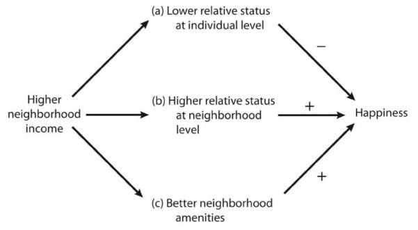
Hypothesized pathways linking neighborhood income to individual happiness
In addition to desiring higher status, individuals desire good schools, well-maintained housing units, a safe environment, and so on, and those amenities covary with neighborhood income in the United States. Hence, even in the presence of strong status effects at the individual level (pathway a in fig. 3), individuals nevertheless might be happier in a richer neighborhood because that effect is more than offset by the greater neighborhood prestige and better collective amenities offered by residence in a richer neighborhood (pathways b and c in fig. 3). That, in fact, is what we hypothesize—that the effects of pathways b and c prevail in figure 3 (or the richer neighbors–greater happiness hypothesis):
Hypothesis
Living in a richer neighborhood has a positive effect on happiness.
Finally, on the basis of figure 3, some readers might wonder why we do not predict that living in a richer county will also have a positive effect on happiness, since pathway c could exist at the county level as well as at the neighborhood level. The answer is that, in the United States at least, pathway c is dramatically weaker at the county level than at the neighborhood level because the collective features that affect happiness tend to vary much more across neighborhoods than across counties. In virtually any U.S. county there are neighborhoods in which houses are well maintained, crime and delinquency are low, and the level of trust is high. There are other neighborhoods in which trust is low; crime and delinquency are high; and unkempt houses, vacant lots, and abandoned buildings dot the landscape. These differences are masked by a measure of overall median county income, but they are largely captured by median income at the neighborhood level since the presence or absence of such amenities is linked closely to income at that geographic scale (Cohen and Dawson 1993; Raudenbush and Sampson 1999; Rankin and Quane 2000; Harding 2003).
We now describe the data and measures we use to test the richer neighbors–greater happiness hypothesis.
DATA AND MEASURES
Studies of Americans’ happiness or life satisfaction (we use the terms interchangeably) typically are based on the GSS.11 We use the 2000 American National Election Study (ANES) because these data contain identifiers (available only under special arrangements with ANES staff) that allowed us to match respondents to block groups and counties. Our study is among the first to estimate income context effects on happiness with nationally representative survey data, and to our knowledge it is the first to estimate income effects at three different levels—household, neighborhood, and county. Our final sample consists of 1,266 individuals spread across 849 neighborhoods (census block groups) in 433 counties.12
Census Data Appended to the ANES
Social scientists who want to study the effects of neighborhood or community context are limited to a relatively short list of data sets, and these data sets often are limited to a single city or region of the country. To obtain a nationally representative sample, it is often necessary to join national survey data to geographic context data from other sources. In this study we append block group–level and county-level income data from the U.S. census to survey data on life satisfaction from the ANES. The ANES contains a sample of noninstitutionalized adults in the contiguous United States, collected every two years around both presidential and midterm elections. Each survey is carried out in two waves, one before the election and one after the election. We use the 2000 ANES because the 2000 survey is the only one that includes both a question about life satisfaction and identifiers for respondents’ neighborhoods. The 2000 ANES has the further advantage of coinciding with the 2000 census, so the conjoined census data reliably reflect the neighborhood and county incomes where the ANES respondents live.
Measure of Happiness
The life satisfaction question in the 2000 ANES is as follows: “In general, how satisfying do you find the way you’re spending your life these days? Would you call it completely satisfying, pretty satisfying, or not very satisfying?” In response, 20.5% said “completely satisfying,” 66.5% said “pretty satisfying,” and 13% said “not very satisfying.”13
A question that naturally arises at this point is whether self-reported measures of happiness or satisfaction can be trusted. A good deal of research supports the view that individuals are in the best position to gauge their own subjective well-being. Konow and Earley (2007, n. 1) cite studies showing that self-reported subjective well-being has positive and generally high correlations with reports of spouses, with recall of positive and negative life events, with the duration of authentic smiles, with heart rate and blood pressure measures of responses to stress, and with skin resistance measures of responses to stress. Because self-reported happiness correlates well with a variety of relevant measures, survey data on happiness or life satisfaction are generally seen as valid (Blanchflower and Oswald 2004; Kahneman and Krueger 2006).
Income Measures
Household income
The ANES includes measures of both household income and personal earnings. In the ANES as well as in the GSS, happiness is more strongly associated with household or family income than with personal earnings. This makes sense: If money is consequential primarily because of what it can do for a person—in terms of either consumption or relative status—then who earns the money is less relevant than how much is earned. (Consistent with this reasoning, we find that work status has little effect on happiness: workers, retirees, and students are equally happy, and those keeping house are, if anything, slightly happier, other things equal [app. table B1]. Only the disabled and the involuntarily unemployed are notably unhappier than workers.) We use household income, then, as our measure of income at the individual level.
The ANES income variable for the 2000 survey consists of 22 response categories, ranging from a 1999 pretax income of less than $5,000 to an income of $200,000 or more. Because accurate measurement of individuals’ household incomes is crucial, we attempted to reduce measurement error as much as possible by making assumptions about the likely distribution of individuals within each category, calculating the mean income of each category under these assumptions and assigning respondents the average income of their category. We follow Jargowsky (1995, 1996) in assuming a uniform distribution for the income categories with lower bounds below the median income and a Pareto distribution for the income categories with lower bounds above the median income. The mean income of the categories that follow a uniform distribution is simply the midpoint of the category, whereas the mean income of the categories that follow a Pareto distribution is calculated using formulas derived by Cloutier (1988) and Jargowsky (1995).14
Income context
We measure income context at the neighborhood level using age-specific median household income for block groups and income context at the county level using age-specific median household income for counties. Recall our theorizing about income effects at the neighborhood level (fig. 3 above). To the extent that neighbors’ income is closely tied to desirable public amenities and to higher neighborhood status (a “better address”), people are happier residing among the rich. Because critical public amenities such as safety vary greatly across U.S. neighborhoods and relatively less across U.S. counties, we hypothesize that the amenities-prestige effect dominates at the local neighborhood level but not at the county level, where we expect Veblen status effects to dominate.
To identify the income comparison groups that matter, we assume that individuals are most likely to compare themselves to the people they are most likely to know, or know about, and consider to be “equals”—those who live in their general region and are at similar stages in the life cycle. Age or life-cycle propinquity is as important to capture as residential propinquity because couples with same-age children tend to intermingle at school, at children’s events, at religious services, and so on; such life-cycle clustering is prominent among younger and older adults as well. Moreover, Americans are in the habit of comparing themselves to their age peers since the age-graded character of the educational system itself conditions Americans to do so.
To model the simultaneous effects of residential and age propinquity, we measure income context using age-specific median income for block groups and counties. The U.S. Census Bureau provides 1999 median household income for counties and block groups broken down by seven age categories: householder is under 25 years, 25–34 years, 35–44 years, 45–54 years, 55–64 years, 65–74 years, and 75 years or older. For our purposes, age-specific median neighborhood income is a better measure than overall median neighborhood income because we assume that the availability of amenities that matter at a particular stage in the life course (e.g., good playgrounds for those with young children, good medical facilities for older residents) is tied more closely to the income of same-age neighbors than to the incomes of much older or younger neighbors. In addition, it is natural to use age-specific incomes to capture Veblen status effects because individuals are most likely to compare their incomes to those of others who are the same age (Firebaugh and Tach, in press).
Control Variables
Americans living in rich and poor places differ on personal characteristics other than income, and those characteristics might account for differences in happiness across neighborhoods and counties. Imagine, for example, that residents of richer neighborhoods tend to be happier only because they are more likely to be married and to have a college education. In this case it would not matter where individuals live or whom they live beside, and the observed association of income context and happiness would disappear if we adequately controlled for marital status and education.
To alleviate this problem, we include controls for key personal characteristics that are associated with happiness: age and age squared, education (four categories), marital status (five categories), work status (six categories, including student status), and race/ethnicity (three categories). Although prior studies find little or no difference in satisfaction between men and women, we also include a dummy variable for gender because of its status as a master variable. On the basis of the findings of prior studies of happiness or life satisfaction in America (e.g., Blanchflower and Oswald 2004; Luttmer 2005; Yang 2008), we expect satisfaction to be positively related to education and to have a U-shaped relationship with age, we expect whites to be more satisfied than nonwhites, we expect those who are married to be more satisfied than those who are not, and we expect those who are unemployed or disabled to be less satisfied.
What about Selection on the Dependent Variable?
There remains the issue of selection effects since unaccounted-for variation in satisfaction across individuals could result in biased estimates of the neighborhood effect if satisfaction itself affects individuals’ decisions about where to live and thus their income context.15 Consider two individuals matched on education, marital status, race, age, income, and so on—two people who, on the basis of our equations, would have the same predicted level of satisfaction. Yet, for whatever reason, one is more satisfied. If, across all such pairs, the more satisfied person is more likely to choose to live in a rich neighborhood, then our estimate of the neighborhood income effect is upwardly biased. Actually, though, the opposite is more plausible: At a given level of income, we expect the chronically dissatisfied to be quicker to move to higher-income areas as income allows and quicker to abandon deteriorating neighborhoods. If in fact dissatisfied people are more prone to move to richer neighborhoods, that would tend to concentrate the dissatisfied in richer neighborhoods and thus bias our estimate of the neighborhood income effect in the negative direction. If anything, then, neighborhood selection would bias results against our hypothesis of a positive effect of neighborhood income on happiness.
ANALYSIS AND RESULTS
Models
We test the richer neighbors–greater happiness hypothesis by measuring income at the household, neighborhood (block group), and county levels. Let H denote happiness, Y denote income, and Z denote the nonincome determinants of happiness. We use subscripts to distinguish income at three nested levels of aggregation: Yijk refers to household income for respondent i in block group j in county k, Yjk refers to age-specific median household income in block group j in county k, and Yk refers to age-specific median household income in county k.
To determine whether results are sensitive to the way we specify the income effects, we estimate two different types of income models. In the first type, happiness is predicted by the level of household income, level of neighborhood income, and level of county income:
| (1) |
We log the income variables because, as in prior studies, we assume that the income-happiness gradient is steeper among the poor than among the rich (an extra $10,000 is unlikely to purchase as much happiness for a millionaire as it would for the average American). As a check for robustness, we also estimated models in which income was not logged (not shown); results are the same. As an additional check we estimated models adjusting for state differences in cost of living (we used the Berry-Fording-Hanson [2000] index); again, the results are the same.
For model (1) we expect the neighborhood income effect to be positive (β2 > 0). In other words, for a given level of household income and other controls, we expect individuals to be happier when they live among affluent neighbors. By contrast, we expect the county income effect to be negative (β3 < 0), reflecting Veblen status effects.
The second type of model expresses incomes as ratios:
| (2) |
Equation (2) uses income ratios formed by dividing household income by the income of a reference group (neighborhood and county, respectively). We follow this strategy to adhere closely to Veblen’s ([1899] 1973) notion that what matters is one’s rank: as Veblen put it, people desire to be rich in order “to rank high in comparison with the rest of the community in point of pecuniary strength” (pp. 39–40; see n. 2 above). The use of ratio variables also helps adjust income for cost-of-living differences across regions of the country since kXijk/kXk = Xijk/Xk (where k is the inflation or deflation factor for living costs).
By using income ratios in equation (2), we reverse the signs of the coefficients. The important point to remember is that we still expect opposing signs at the neighborhood and county levels. The richer neighbors–greater happiness hypothesis postulates that, whatever one’s income, one is happier in the midst of rich neighbors, so the coefficient for the ratio of one’s income to the average income in the neighborhood, Yijk/Yjk, should be negative in equation (2). The Veblen status effect at the county level implies, by contrast, that one is happier in a poor county, so the coefficient for Yijk/Yk should be positive.
We estimated the effect of neighborhood and county income on happiness using ordered logit models. Because the dependent variable consists of three response categories, we first tested the proportional odds assumption that the effect of a $1,000 increase in household income on having a “completely satisfying” or “pretty satisfying” life rather than a “not very satisfying” one is identical to the effect of a $1,000 increase in household income on having a “completely satisfying” life rather than a “pretty satisfying” or “not very satisfying” one (and similarly for the effects of the other independent variables). Tests of that assumption using the gologit2 program for Stata (Williams 2006) indicated that it holds for our analysis. Thus our results can be reported parsimoniously with a single coefficient for each regressor as opposed to separate coefficients for the comparisons “completely satisfying versus otherwise” and “not very satisfying versus otherwise.”
Results
The first step is to verify that happiness is associated with household, neighborhood, and county income in the directions predicted: namely, (1) richer people tend to be happier, independent of where they live; (2) people in richer neighborhoods tend to be happier, net of the effect of their own income; and (3) people in poorer counties tend to be happier, net of the effect of their own income.
The ANES data strongly confirm each of the associations (cols. 1 and 2 of table 1). Richer people tend to be happier, controlling for neighborhood and county income. Residents of richer neighborhoods tend to be happier, controlling for own income and county income. Residents of poorer counties tend to be happier, controlling for own income and neighborhood income.
TABLE 1.
Estimated Effects of Neighborhood and County Income on Life Satisfaction
| Income Variables Only |
Controlling for Respondent’s Non- income Characteristics |
|||
|---|---|---|---|---|
| Logit (1) |
SE (2) |
Logit (3) |
SE (4) |
|
| Income effects at three levels: | ||||
| Household income, log(Yijk) . . . . . . . . . | .279** | .083 | .056 | .098 |
| Median neighborhood income, log(Yjk) . . . . . . . . . . . . . . . . . . . . . . . . . . . . . . |
.447** | .123 | .305* | .132 |
| Median county income, log(Yk) . . . . . | −1.028** | .238 | −.386† | .246 |
| Pseudo R2 . . . . . . . . . . . . . . . . . . . . . . . . . . . . | .019 | .058 | ||
| Income measured as ratio: | ||||
| Household-neighborhood ratio, Yijk/Yjk . . . . . . . . . . . . . . . . . . . . . . . . . . . . . . |
−4.003** | 1.150 | −2.672* | 1.270 |
| Household-county income ratio, Yijk/Yk . . . . . . . . . . . . . . . . . . . . . . . . . . . . . . . |
7.234** | 1.267 | 3.471* | 1.477 |
| Pseudo R2 . . . . . . . . . . . . . . . . . . . . . . . . . . . . | .023 | .058 | ||
Note.–The sample consists of 1,266 individuals in 849 neighborhoods (census block groups) and 433 counties. The variable Yijk is household income for respondent i in block group j in county k. Incomes below the median have been assigned using linear interpolation between the category boundaries; incomes above the median have been assigned by fitting them to a Pareto distribution. Median county income and median neighborhood income are age specific to capture age propinquity as well as residential propinquity. All models include a dummy variable for sampling design (face-to-face vs. phone interview); those coefficients are always minuscule and are not reported here. The other nonincome control variables are age and age squared, gender, education, race/ethnicity, work status, and marital status. Appendix table B1 reports coefficients for the nonincome variables for the top model above, and app. table B2 reports means and correlations of the income variables for the top model.
P = .12 (two-tailed tests; SEs corrected for clustering).
P < .05.
P < .01.
We reach the same conclusions when incomes are measured as ratios. For a given level of income, Americans tend to be happier when they live in rich neighborhoods (the coefficient for Yijk/Yjk is negative) in poor counties (the coefficient for Yijk/Yk is positive). Although Americans are happier when their nearby neighbors are well off, that amenities-prestige effect does not carry over to the county level. Instead Veblen status effects appear to dominate at the county level.
The next step is to add control variables to determine whether the observed differences in happiness across neighborhoods and counties reflect context effects—the difference a place makes—or merely variation in the characteristics of people in each place (composition effects). The issue is important. If income context itself matters, then we can expect individuals’ levels of happiness to change when they move to different income contexts. However, if composition effects account for residential variations in happiness, then individuals’ happiness will be the same regardless of where they live.
Columns 3 and 4 of table 1 report the income results for the full models. Clearly factors other than income affect happiness, as indicated by the increase in R2 when the nonincome variables are added in table 1. (Appendix table B1 reports coefficients for the nonincome variables.) We expect income coefficients in table 1 to diminish if only because some of the control variables constitute pathways through which income affects happiness (e.g., if higher income enables marriage and marriage boosts happiness, then part of the causal effect of own income on happiness is removed by controlling for marriage), so our results likely provide conservative estimates of the causal effect of income on happiness
We find that household income has no statistically significant effect on happiness net of the effects of marital and work status, education, gender, race, age, and county and neighborhood income. Apparently the difference in happiness between the rich and the poor (as seen, e.g., in fig. 1) can be accounted for by differences in education, marital status, neighborhood income, and so on.16
Net of the controls, the estimated effect of county income on happiness remains statistically significant (P < .05) in the ratio version of the model but falls short of the conventional .05 criterion when county income is entered as a separate variable. Other models (not shown) consistently indicate a negative effect for county income. Taken as a whole, our findings provide at least qualified support for the relative income idea that there is satisfaction to be gained from residing in a poorer region.17
There is satisfaction to be gained, that is, as long as the poor do not live nearby. That qualification—as long as the poor do not live nearby—is indicated by results for our most critical coefficient: the coefficient for neighborhood income. The neighborhood effect is positive18 and statistically significant with or without controls for respondents’ nonincome characteristics. In short, the ANES data support the richer neighbors–greater happiness hypothesis.
To better gauge the size of the neighborhood income effect, we converted logit coefficients to probabilities for the first model in table 1, holding all other variables at their mean. Figure 4 depicts those results. On the basis of our estimates, residents of low-income neighborhoods are about equally split on the “completely satisfied” and “not very satisfied” responses. But residents of high-income neighborhoods are about twice as likely to say that they are completely satisfied as they are to say that they are not very satisfied.
Fig. 4.

Effect of neighborhood income on satisfaction
It is instructive to compare the size of this neighborhood income effect with the sizes of the effects of selected individual-level characteristics that also predict satisfaction in our models. Other things equal, the largest differences in satisfaction are between married and unmarried individuals, between the involuntarily unemployed or disabled and those working now, and between those who have a high school diploma and those who do not (app. table B1).
The bar graphs in figure 5 depict those differences. Because conclusions are similar for “completely satisfied” and “not very satisfied,” to save space we report only the former. The first pair of bars reproduces the findings for “completely satisfied” in figure 4, this time in the form of a bar graph. The next bars depict the effects of education, unemployment, and marriage, respectively, on satisfaction. The odds of being completely satisfied for people whose neighborhood has a high median income (95th percentile) are 1.8 times the odds of being completely satisfied for people whose neighborhood has a low median income (5th percentile). The comparable odds ratios for the other comparisons (college vs. less than high school, working vs. unemployed, and married vs. divorced) are 2.3, 2.6, and 1.9, respectively. So, in a comparison of the richest versus the poorest 5% of neighborhoods, the neighborhood income effect is comparable to the effect of being married as opposed to being divorced.
Fig. 5.

Effect of neighborhood income versus effects of selected individual characteristics on life satisfaction.
It is important, then, not to exaggerate the effect of neighborhood income on happiness. But neither should the effect be minimized. Even after statistical controls for household income, marital status, work status, education, race, age, and gender, those living in high-income neighborhoods are about 50% more likely to say that they are completely satisfied with life (fig. 5)—and about one-third less likely to say that they are not very satisfied (not shown)—than those living in low-income neighborhoods.
SUMMARY AND IMPLICATIONS
Thomas Carlyle ([1843] 2005, p. 155) wrote that “every pitifulest whipster that walks within a skin has his head filled with the notion that he is, shall be, or by all human and divine laws ought to be, ‘happy.’” According to the relative income hypothesis, prominently featured in social science but rarely tested, higher income will make Carlyle’s pitifulest whipster happier, but only at the expense of others’ happiness.
The central (and new) finding in this study is that the relative income hypothesis does not apply at the neighborhood level. Net of the effects of own income, Americans tend to be happier when their nearby neighbors are rich, not poor. This is not to say that people fail to compare their incomes to their neighbors’ incomes, but it is to say that the negative effect of one’s lower relative status in a richer neighborhood is more than offset by the positive effect of the better amenities and higher prestige associated with a richer neighborhood. At the neighborhood level, then, Veblen status effects apparently are submerged by the positive effects of residence in richer neighborhoods.
At the county level, by contrast, we do find evidence consistent with the relative income hypothesis. The practical and theoretical implications of relative income effects are far-reaching (Frank 1999; Firebaugh 2008, pp. 54–56). If relative income were the sole determinant of happiness, middle-income Americans of the 19th century—who owned neither automobiles nor air conditioners nor color televisions—must have been as happy as middle-income Americans are today. And if in the future everyone else owns a Rolls Royce, we will be unhappy with a Lexus.
We can now answer the question posed by the article’s title: Yes, your neighbor’s income does affect your happiness, but the income of your proximate neighbor has a different effect on your happiness than the income of your more distant neighbor does. Americans tend to be happiest when they live in a high-income neighborhood in a low-income region. In other words, the effect of residential income on individual happiness reverses from positive to negative with increasing geographic scale—a phenomenon we might call the geographic scale principle of income effects (Lee et al. [2008] argue, along the same vein, that the effect of residential segregation can vary by geographic scale).
The geographic scale principle of income effects implies that individuals are happier when they live among the poor, as long as the poor reside at a distance. Is that a general principle for humans? Subsequent analyses are needed, and we look forward to studies using data sets for other countries to investigate the generality issue as well as to studies using other U.S. data sets to verify the ANES results we report here.
We end by considering how our results bear on the Easterlin paradox and on the neighborhood effects literature. Note that if, as the scale principle of income effects suggests, Veblen status effects dominate the income-happiness association at the supraneighborhood level, Veblen status effects could prevail at the national level, thus accounting for the failure of national happiness to rise with national income. Hence our findings are quite consistent with the relative income explanation of the Easterlin paradox.
With respect to the literature on neighborhood effects, our results for happiness replicate and extend research on the negative consequences of living in poor neighborhoods. As noted earlier, prior neighborhood studies document the effects of neighborhood income on more or less objective conditions such as crime, school dropout rates, and rates of teenage pregnancy. The results here extend those findings by showing that poor neighborhoods depress their residents’ subjective well-being as well. While these less tangible neighborhood effects have not received much attention from researchers, they represent another real cost of living among concentrated poverty and therefore deserve more consideration.
APPENDIX A. Sampling Issues in the 2000 ANES
A possible problem with using the 2000 ANES is that this version of the ANES experimented with drawing respondents from two different sampling frames and used different interview methods (face-to-face vs. telephone interviews). The first method used a traditional multistage probability sample design to select respondents for in-home interviews. The second method used random digit dialing to select respondents, and all interviews were conducted over the telephone.
Because we worried that this hybrid methodology would affect our results, we included a dummy variable in all models to distinguish face-to-face interviews from the phone interviews; its coefficient was minuscule. In supplemental analyses (not shown), we also used interaction terms formed by multiplying the key independent variables by the dummy variable to examine whether the effects of income context differed by sample type. The coefficients for all interaction terms fell well short of statistical significance. Thus our concerns proved unfounded: The hybrid sampling methodology does not influence our results.
APPENDIX B
TABLE B1.
Determinants of Life Satisfaction: Coefficients for Control Variables
| Logit | SE | |
|---|---|---|
| Age . . . . . . . . . . . . . . . . . . . . . . . . . . . . . . . . . . . . . . . . . . . . . . . . . . . . . . . . . . . . . . | .009 | .006 |
| Age2/100 . . . . . . . . . . . . . . . . . . . . . . . . . . . . . . . . . . . . . . . . . . . . . . . . . . . . . . . . . | .084* | .033 |
| Gender (1 = male) . . . . . . . . . . . . . . . . . . . . . . . . . . . . . . . . . . . . . . . . . . . . . | .060 | .126 |
| Education: | ||
| No high school diploma (reference) . . . . . . . . . . . . . . . . . . . . . . . . | ||
| High school diploma . . . . . . . . . . . . . . . . . . . . . . . . . . . . . . . . . . . . . . . . | .592* | .249 |
| Junior college degree . . . . . . . . . . . . . . . . . . . . . . . . . . . . . . . . . . . . . . . . | .861** | .310 |
| College/graduate degree . . . . . . . . . . . . . . . . . . . . . . . . . . . . . . . . . . . . . | .843** | .291 |
| Race/ethnicity: | ||
| White (reference) . . . . . . . . . . . . . . . . . . . . . . . . . . . . . . . . . . . . . . . . . . . . . | ||
| Black . . . . . . . . . . . . . . . . . . . . . . . . . . . . . . . . . . . . . . . . . . . . . . . . . . . . . . . . . . | −.276 | .206 |
| Other . . . . . . . . . . . . . . . . . . . . . . . . . . . . . . . . . . . . . . . . . . . . . . . . . . . . . . . . . . | .150 | .219 |
| Work status: | ||
| Working or temporarily laid off (reference) . . . . . . . . . . . . . . . | ||
| Unemployed . . . . . . . . . . . . . . . . . . . . . . . . . . . . . . . . . . . . . . . . . . . . . . . . . . | −.964* | .378 |
| Retired . . . . . . . . . . . . . . . . . . . . . . . . . . . . . . . . . . . . . . . . . . . . . . . . . . . . . . . . | −.004 | .287 |
| Permanently disabled . . . . . . . . . . . . . . . . . . . . . . . . . . . . . . . . . . . . . . . | −.774* | .359 |
| Keeping house . . . . . . . . . . . . . . . . . . . . . . . . . . . . . . . . . . . . . . . . . . . . . . . | .499† | .271 |
| Student . . . . . . . . . . . . . . . . . . . . . . . . . . . . . . . . . . . . . . . . . . . . . . . . . . . . . . . | −.090 | .437 |
| Marital status: | ||
| Married (reference) . . . . . . . . . . . . . . . . . . . . . . . . . . . . . . . . . . . . . . . . . . | ||
| Widowed . . . . . . . . . . . . . . . . . . . . . . . . . . . . . . . . . . . . . . . . . . . . . . . . . . . . . | −.155 | .264 |
| Divorced . . . . . . . . . . . . . . . . . . . . . . . . . . . . . . . . . . . . . . . . . . . . . . . . . . . . . . | −.625** | .196 |
| Separated . . . . . . . . . . . . . . . . . . . . . . . . . . . . . . . . . . . . . . . . . . . . . . . . . . . . . | −.855** | .304 |
| Never married/cohabiting . . . . . . . . . . . . . . . . . . . . . . . . . . . . . . . . . . . | −.459** | .167 |
| Dummy for sampling method (1 = face-to-face) . . . . . . . . . . . | −.021 | .114 |
| Thresholds: | ||
| “Completely satisfied” or “pretty satisfied” vs. “not very satisfied” . . . . . . . . . . . . . . . . . . . . . . . . . . . . . . . . . . . . . . . . . . . . . . . . . . . |
−1.261 | |
| “Completely satisfied” vs. “pretty satisfied” or “not very satisfied” . . . . . . . . . . . . . . . . . . . . . . . . . . . . . . . . . . . . . . . . . . . . . . . . . . . |
2.314 | |
| Pseudo R2 . . . . . . . . . . . . . . . . . . . . . . . . . . . . . . . . . . . . . . . . . . . . . . . . . . . . . . . | .058 |
Note.–This table reports results for nonincome coefficients for the first model in table 1 of the text. Similar results hold for the income ratio model in table 1. The sample consists of 1,266 individuals in 849 neighborhoods (census block groups) and 433 counties. See the note to table 1 for further details.
P < .10 (two-tailed tests; SEs corrected for clustering).
P < .05.
P < .01.
TABLE B2.
Descriptive Statistics and Correlations for Logged Income Variables (N = 1,266 Individuals)
| Mean | SD | (1) | (2) | (3) | |
|---|---|---|---|---|---|
| 1. Individual income, log(Yijk) . . . . . | 10.56 | .90 | … | ||
| 2. Median neighborhood income, log(Yjk) . . . . . . . . . . . . . . . . . . . . . . . . . . . . . |
10.64 | .61 | .44 | … | |
| 3. Median county income, log(Yk) . . . . . . . . . . . . . . . . . . . . . . . . . . . . . |
10.71 | .38 | .37 | .63 | … |
Footnotes
This article is based on work supported by the National Science Foundation under grant 0549718 to Firebaugh. We thank officials at the American National Election Study for permission to use restricted information needed for the contextual analysis done here. We also thank Lori Burrington, Michael Massoglia, Eric Silver, Laura Tach, and the AJS reviewers for comments.
We use the term “Veblen status effects” as shorthand for the condition in which a person’s own status is diminished by the high status of others—Veblen’s ([1899] 1973) core argument about income effects. What matters most is income or wealth rank. Where there is private property, Veblen declares that “the end sought by accumulation is to rank high in comparison with the rest of the community in point of pecuniary strength. … Relative success, tested by an invidious pecuniary comparison with other men, becomes the conventional end of action” (pp. 39–40).
There is a large and growing sociological literature on neighborhood effects, but those studies focus on the effects of neighborhood context on outcomes such as crime, teenage pregnancy, educational attainment, and so on rather than on the effect of neighborhood income on happiness or subjective well-being (see Sampson, Morenoff, and Gannon-Rowley [2002] for a review).
The finding that happier nuns lived longer is all the more compelling because of the homogeneity of the subjects: They were all female, they had the same reproductive and marital histories, they had access to the same medical care, they did not smoke, they did not drink alcohol in excess, they did similar work, they lived in the same environs, and they had almost exactly the same occupation and socioeconomic status.
Over the period 2001–5, economists produced more than 100 papers analyzing data on self-reported life satisfaction or happiness. A decade earlier, from 1991 to 1995, economists had produced only four such papers (Kahneman and Krueger 2006, p. 3). The study of happiness has a longer history in psychology, of course (Argyle 1987). For an overview of how happiness has been viewed historically by philosophers and others, see McMahon (2006).
Happiness is coded on a three-point scale, where 1 signifies “not too happy” and 3 signifies “very happy.” Despite the large sample, the slope for happiness in fig. 2 is not close to being statistically significant. Ordered logit methods produce the same results; i.e., happiness has not risen in America (Yang 2008).
According to Layard (2005, pp. 3–4), “As Western societies have got richer, their people have become no happier. … This devastating fact should be the starting point for all discussion of how to improve our lot.” In a contrary view, Stevenson and Wolfers (2008) argue that happiness generally has risen with economic growth in the West.
Note the possible radical implication of this statement for the discipline of economics: If economic growth per se is of little importance for human happiness, then it should be abandoned as the primary objective of economic policy (Oswald 1997). It is not surprising, then, that the study of human happiness has become a major topic in economics (Clark et al. 2008).
Fischer (2008) notes that median household incomes rose only because Americans (especially women) worked more hours on average; mean hourly wages did not rise. For him, it thus makes sense that happiness would likewise not rise. In separate analyses (not shown), however, we find that total household income matters more for happiness than respondent’s income does. Nor does work status (employed, retired, housewife, or student) have much effect on happiness. Hence the negative consequence of increased time spent at work for household members collectively appears not to offset the positive effect of increased household income on happiness.
The concept of “community” means different things to different people. We use the term only as shorthand for a geographic area bigger than a neighborhood and make no claims that people actually think of counties as their “community.”
Although satisfaction might be conceptualized as a more enduring state than happiness, questions using the terms “happy” and “satisfied” to describe overall life condition typically yield the same conclusions; so the terms are viewed as equivalent, or nearly so, in most survey research.
Studies of neighborhood effects in the United States generally are based on census tracts or block groups. The U.S. Census Bureau divides counties into census tracts that are in turn subdivided into block groups of about 1,400 people. We use the block group to measure the income of nearby neighbors because it is the smallest spatial unit for which the Census Bureau reports median household income.
Compare these figures with the GSS, where about 30% of respondents say that they are “very happy,” about 57% say that they are “pretty happy,” and about 13% say that they are “not too happy.” Note that both the ANES and the GSS ask respondents to rate their satisfaction or happiness with life in general, not their satisfaction or happiness with their income. Although the two issues may be related, they should not be confused. Another line of research in the social sciences—called the distributive justice literature (e.g., Jasso 1978; Alwin 1987)—addresses the issue of people’s satisfaction with their income (i.e., on whether they perceive their income as fair).
The Pareto distribution has a long right tail, which reflects the skewness of the American income distribution. Were we to ignore the likely skewness of the ANES income distribution by simply assigning all respondents the midpoint of their income category, we would overestimate the incomes of individuals in categories above the median. Additionally, the procedure we use yields a more informed estimate of the average income of the unbounded top category, which must otherwise be arbitrarily assigned.
Satisfaction might also affect individual income—happier people make more money—but that does not pose a problem since we control for individual income in our models. With respect to the selection bias issue for income context, note that life satisfaction was measured in 2000, whereas neighborhood and community income is for 1999.
If so, the consumption-related reason richer Americans are happier than poorer Americans perhaps has less to do with differences in the consumption of consumer goods and more to do with “consumption” differences in the education, marriage, and real estate markets: higher income is associated with more education, with marriage, and with living in a more affluent neighborhood. We cannot pursue the issue here because we lack measures of material possessions.
One reviewer argued strongly that, since we had adequate theoretical justification for predicting the direction of the income effects, we should use one-tailed tests for our income coefficients. On the basis of one-tailed tests, the estimated effect of county income is statistically significant at P < .01 in the ratio version of the model and marginally not significant (P = .058) when county income is entered as a separate variable. Rather than relying on an arbitrary cutoff point such as P < .05 to determine the level of confidence to place in findings, we agree with Leamer (1985) that it is more telling to consider the robustness of the results across alternative specifications. In brief, the effect of county income on happiness is always negative and usually significant (under either one- or two-tailed tests) whether we log income or use untransformed income, whether we enter income as separate variables or use ratios, whether we use household income or personal income as our measure of income at the individual level, whether or not we adjust for cost-of-living differences across regions, and whether or not we control for possible effects of the ANES sampling design (results available on request).
Recall that a negative coefficient for the household-neighborhood ratio indicates a positive neighborhood income effect.
Contributor Information
Glenn Firebaugh, Pennsylvania State University.
Matthew B. Schroeder, University of Minnesota
REFERENCES
- Alwin Duane. Distributive Justice and Satisfaction with Material Well-Being. American Sociological Review. 1987;52:83–95. [Google Scholar]
- Argyle Michael. The Psychology of Happiness. Routledge; New York: 1987. [Google Scholar]
- Berry William D., Fording Richard C., Hanson Russell L. An Annual Cost of Living Index for the American States, 1960–1995. Journal of Politics. 2000;62:550–67. [Google Scholar]
- Blanchflower David G., Oswald Andrew J. Well-Being over Time in Britain and the USA. Journal of Public Economics. 2004;88:1359–86. [Google Scholar]
- Brickman Philip, Campbell Donald T. Hedonic Relativism and Planning the Good Society. In: Appley MH, editor. Adaptation-Level Theory: A Symposium; New York: Academic Press; 1971. pp. 287–302. [Google Scholar]
- Carlyle Thomas. Past and Present. University of California Press; Berkeley and Los Angeles: 2005. (1843) [Google Scholar]
- Clark Andrew E., Frijters Paul, Shields Michael A. Relative Income, Happiness, and Utility: An Explanation for the Easterlin Paradox and Other Puzzles. Journal of Economic Literature. 2008;46:95–144. [Google Scholar]
- Cloutier Norman R. Pareto Extrapolation Using Grouped Income Data. Journal of Regional Science. 1988;28:415–19. [Google Scholar]
- Cohen Cathy J., Dawson Michael C. Neighborhood Poverty and African American Politics. American Political Science Review. 1993;87:286–302. [Google Scholar]
- Csikszentmihalyi Mihaly. Flow: The Psychology of Optimal Experience. Harper & Row; New York: 1990. [Google Scholar]
- Danner Deborah D., Snowdon David A., Friesen Wallace C. Positive Emotions in Early Life and Longevity: Findings from the Nun Study. Journal of Personality and Social Psychology. 2001;80:804–13. [PubMed] [Google Scholar]
- Diener Edward, Suh Eunkook M., Lucas Richard E., Smith Heidi L. Subjective Well-Being: Three Decades of Progress. Psychological Bulletin. 1999;125:276–303. [Google Scholar]
- Duesenberry James. Income, Savings, and the Theory of Consumer Behavior. Harvard University Press; Cambridge, Mass.: 1949. [Google Scholar]
- Durkheim Émile. Suicide: A Study in Sociology. Free Press; Glencoe, Ill.: 1958. (1897) [Google Scholar]
- Easterlin Richard A. Does Money Buy Happiness? Public Interest. 1973;30:3–10. [Google Scholar]
- — — — . Does Economic Growth Improve the Human Lot? Some Empirical Evidence. In: David PA, Reder MW, editors. Nations and Households in Economic Growth: Essays in Honour of Moses Abramovitz. Academic Press; New York: 1974. pp. 89–125. [Google Scholar]
- — — — Will Raising the Incomes of All Increase the Happiness of All? Journal of Economic Behavior and Organizations. 1995;27:35–48. [Google Scholar]
- — — — . Growth Triumphant: The Twenty-first Century in Historical Perspective. University of Michigan Press; Ann Arbor: 1996. [Google Scholar]
- — — — Income and Happiness: Towards a Unified Theory. Economic Journal. 2001;111:465–84. [Google Scholar]
- — — — Feeding the Illusion of Growth and Happiness: A Reply to Hagerty and Veenhoven. Social Indicators Research. 2005;74:429–43. [Google Scholar]
- Elster Jon, Roemer John E., editors. Interpersonal Comparisons of Well-Being. Cambridge University Press; Cambridge: 1991. [Google Scholar]
- Ferrer-i-Carbonell Ada. Income and Well-Being: An Empirical Analysis of the Comparison Income Effect. Journal of Public Economics. 2005;89:997–1019. [Google Scholar]
- Firebaugh Glenn. Seven Rules for Social Research. Princeton University Press; Princeton, N.J.: 2008. [Google Scholar]
- Firebaugh Glenn, Tach Laura. Income and Happiness: Are Americans on a Hedonic Treadmill? In: Marsden Peter V., editor. Social Trends in the United States, 1972–2006: Evidence from the General Social Survey. Princeton University Press; Princeton, N.J.: In press. [Google Scholar]
- Fischer Claude. What Wealth-Happiness Paradox? A Short Note on the American Case. Journal of Happiness Studies. 2008;9:219–26. [Google Scholar]
- Frank Robert H. Choosing the Right Pond: Human Behavior and the Quest for Status. Oxford University Press; Oxford: 1985. [Google Scholar]
- — — — . Luxury Fever: Why Money Fails to Satisfy in an Era of Excess. Free Press; New York: 1999. [Google Scholar]
- Frey Bruno S., Stutzer Alois. What Can Economists Learn from Happiness Research? Journal of Economic Literature. 2002;40:402–35. [Google Scholar]
- Gilbert Daniel. Stumbling on Happiness. Knopf; New York: 2006. [Google Scholar]
- Hagerty Michael R. Social Comparisons of Income in One’s Community: Evidence from National Surveys on Income and Happiness. Journal of Personality and Social Psychology. 2000;78:764–71. doi: 10.1037//0022-3514.78.4.764. [DOI] [PubMed] [Google Scholar]
- Haidt Jonathan. The Happiness Hypothesis. Basic Books; New York: 2006. [Google Scholar]
- Harding David J. Counterfactual Models of Neighborhood Effects: The Effect of Neighborhood Poverty on Dropping Out and Teenage Pregnancy. American Journal of Sociology. 2003;109:676–719. [Google Scholar]
- Helson Harry. Adaptation-Level Theory. Harper & Row; New York: 1964. [Google Scholar]
- Jargowsky Paul A. Take the Money and Run: Economic Segregation in U.S. Metropolitan Areas. University of Wisconsin—Madison, Institute for Research on Poverty; 1995. Discussion Paper no. 1056-95. [Google Scholar]
- — — — Take the Money and Run: Economic Segregation in U.S. Metropolitan Areas. American Sociological Review. 1996;61:984–98. [Google Scholar]
- Jasso Guillermina. On the Justice of Earnings: A New Specification of the Justice Evaluation Function. American Journal of Sociology. 1978;83:1398–1419. [Google Scholar]
- Kahneman Daniel, Diener Ed, Schwarz Norbert., editors. Well-Being: The Foundations of Hedonic Psychology. Russell Sage Foundation; New York: 2003. [Google Scholar]
- Kahneman Daniel, Krueger Alan B. Developments in the Measurement of Subjective Well-Being. Journal of Economic Perspectives. 2006;20:3–24. [Google Scholar]
- Klein Stefan. In: The Science of Happiness: How Our Brains Make Us Happy—and What We Can Do to Get Happier. Lehmann Stephen., editor. Marlowe; New York: 2006. [Google Scholar]
- Koivumaa-Honkanen H, Honkanen R, Koskenvuo M, Kaprio J. Self-Reported Happiness in Life and Suicide in Ensuing 20 Years. Social Psychiatry and Psychiatric Epidemiology. 2003;38:244–48. doi: 10.1007/s00127-003-0625-4. [DOI] [PubMed] [Google Scholar]
- Konow James, Earley Joseph. The Hedonistic Paradox: Is Homo Economicus Happier? 2007 MPRA Paper no. 2728. http://mpra.ub.uni-muenchen.de/2728/
- Layard Richard. Happiness: Lessons from a New Science. Penguin; New York: 2005. [Google Scholar]
- Leamer Edward E. Sensitivity Analyses Would Help. American Economic Review. 1985;75:308–13. [Google Scholar]
- Lee Barrett, Reardon Sean, Firebaugh Glenn, Farrell Chad R., Matthews Stephen A., O’Sullivan David. Beyond the Census Tract: Patterns and Determinants of Racial Segregation at Multiple Geographic Scales. American Sociological Review. 2008;72:766–91. doi: 10.1177/000312240807300504. [DOI] [PMC free article] [PubMed] [Google Scholar]
- Luttmer Erzo. Neighbors as Negatives: Relative Earnings and Well-Being. Quarterly Journal of Economics. 2005;120:963–1002. [Google Scholar]
- Lykken David, Tellegen A. Happiness Is a Stochastic Phenomenon. Psychological Science. 1996;7:186–89. [Google Scholar]
- McMahon Darrin M. Happiness: A History. Grove/Atlantic; New York: 2006. [Google Scholar]
- Morris Martina, Western Bruce. U.S. Earnings Inequality at the Close of the 20th Century. Annual Review of Sociology. 1999;25:623–57. [Google Scholar]
- Nettle Daniel. Happiness: The Science behind Your Smile. Oxford University Press; Oxford: 2006. [Google Scholar]
- Oswald Andrew J. Happiness and Economic Performance. Economic Journal. 1997;107:1815–31. [Google Scholar]
- Rankin Bruce H., Quane James M. Neighborhood Poverty and the Social Isolation of Inner-City African American Families. Social Forces. 2000;79:139–64. [Google Scholar]
- Raudenbush Stephen W., Sampson Robert J. Ecometrics: Toward a Science of Assessing Ecological Settings, with Application to the Systematic Social Observation of Neighborhoods. Sociological Methodology. 1999;29:1–41. [Google Scholar]
- Sampson Robert J., Morenoff Jeffrey D., Gannon-Rowley Thomas. Assessing ‘Neighborhood Effects’: Social Processes and New Directions in Research. Annual Review of Sociology. 2002;28:443–78. [Google Scholar]
- Schnittker Jason. Happiness and Success: Genes, Families, and the Psychological Effects of Socioeconomic Position and Social Support. American Journal of Sociology. 2008;114(suppl.):S233–S259. doi: 10.1086/592424. [DOI] [PubMed] [Google Scholar]
- Seligman Martin. Authentic Happiness: Using the New Positive Psychology to Realize Your Potential for Lasting Fulfillment. Free Press; New York: 2002. [Google Scholar]
- Stevenson Betsey, Wolfers Justin. Economic Growth and Subjective Well-Being: Reassessing the Easterlin Paradox. University of Pennsylvania, Wharton School; 2008. Manuscript. [Google Scholar]
- Veblen Thorsten. The Theory of the Leisure Class: An Economic Study in the Evolution of Institutions. Houghton Mifflin; Boston: 1973. (1899) [Google Scholar]
- Veenhoven Ruut. World Database of Happiness. Erasmus University Rotterdam; Rotterdam: 2008. http://worlddatabaseofhappiness.eur.nl. [Google Scholar]
- Williams Richard. Generalized Ordered Logit/Partial Proportional Odds Models for Ordinal Dependent Variables. Stata Journal. 2006;6:58–82. [Google Scholar]
- Yang Yang. Social Inequalities in Happiness in the United States, 1972–2004: An Age-Period-Cohort Analysis. American Sociological Review. 2008;73:204–226. [Google Scholar]