

Abstract
When mutation rates are low, natural selection remains effective, and increasing the mutation rate can give rise to an increase in adaptation rate. When mutation rates are high to begin with, however, increasing the mutation rate may have a detrimental effect because of the overwhelming presence of deleterious mutations. Indeed, if mutation rates are high enough: (i) adaptive evolution may be neutralized, resulting in a zero (or negative) adaptation rate despite the continued availability of adaptive and/or compensatory mutations, or (ii) natural selection may be neutralized, because the fitness of lineages bearing adaptive and/or compensatory mutations—whether established or newly arising—is eroded by excessive mutation, causing such lineages to decline in frequency. We apply these two criteria to a standard model of asexual adaptive evolution and derive mathematical expressions—some new, some old in new guise—delineating the mutation rates under which either adaptive evolution or natural selection is neutralized. The expressions are simple and require no a priori knowledge of organism- and/or environment-specific parameters. Our discussion connects these results to each other and to previous theory, showing convergence or equivalence of the different results in most cases.
Keywords: population genetics, mutagenesis, error threshold, Fisher's fundamental theorem, beneficial mutations
1. Introduction
Even the simplest of living organisms are highly complex. Mutations—indiscriminate alterations of such complexity—are much more likely to be harmful than beneficial [1–3]. For an individual organism, therefore, an increase in the overall rate of mutation should be detrimental. In a population of organisms, however, natural selection disproportionately favours beneficial mutations, and the net effect of increasing the overall mutation rate is thus less clear.
1.1. Previous studies
Generally speaking, the population-level effects of increasing the mutation rate have been studied separately under two artificial assumptions: the absence of beneficial mutations, and infinite population size. Only a handful of studies have relaxed both assumptions.
1.1.1. Absence of beneficial mutations
When beneficial mutations are assumed to be absent, and population size is finite, fitness will undergo a slow but steady decline because of the sluggish but largely irreversible accumulation of deleterious mutations. This process is especially pronounced in asexual populations, and it was in this context that the process was first described by Muller [4] and later dubbed ‘Muller's ratchet’ [5] and formalized by Haigh [6]. Under the relentless accumulation of deleterious mutations, fitness will decline monotonically. Most of the subsequent work on Muller's ratchet has focused on the rate of the ratchet, different factors affecting this rate, and in particular factors or conditions that can cause this rate to become negligible (i.e. that halt the ratchet) [7–15]. Increasing the genomic mutation rate can only accelerate Muller's ratchet.
1.1.2. Infinite population size
When population size is assumed to be infinite, populations whose adaptation is constrained, i.e. populations in which beneficial mutations can occur but that have a maximum attainable fitness, will eventually achieve an equilibrium fitness distribution shaped by the largely opposing forces of mutation and natural selection. Above a critical mutation rate dubbed the ‘error threshold’ [16,17], this distribution becomes remarkably flat, indicating that a genotype's equilibrium frequency is essentially independent of its fitness. This conversion to a state of random fitness dispersion is reminiscent of a phase transition [17–21] and, in its simplest formulation, the two are mathematically equivalent [22,23]. The simplest formulation of the error threshold has been called into question because of some unrealistic assumptions that are often perceived as strong assumptions, the most notable of which is the ‘single-peak’ fitness landscape assumption [24]. The error threshold has since been studied extensively and shown to exist under many different conditions that eliminate different assumptions, for example, allowing for recombination and departures from random mating [25–27], viral complementation [28], spatial structure and different modes of replication [29–34] and more realistic static and dynamic fitness landscapes [26,27,35–40] (but see Wiehe [41]).
1.1.3. Extinction
The two classes of models described earlier—Muller's ratchet and the error threshold—encompass most previous characterizations of mutational degradation processes. In their original formulations, and in most subsequent work, neither of these two classes of models explicitly accounts for demographic decline as a result of excess mutation. There has been some work, however, that has superimposed demography onto both Muller's ratchet [42–44] and error threshold [45,46] models, finding a positive feedback between these processes and demographic decline towards extinction. These models, however, are typically sensitive to organism-, environment- and time-dependent parameters. In particular, they require an assumption about the mapping between relative and absolute fitness—an assumption that is loaded with requisite assumptions about the organism and environment, both of which can change with time.
1.1.4. Finite populations with beneficial mutations
A few studies have addressed the effect of increasing the mutation rate when the two foregoing assumptions are relaxed, i.e. when beneficial mutations are accounted for and populations are finite. Under these more realistic conditions, the fitness decline due to Muller's ratchet can be cancelled out or even reversed by beneficial mutations, resulting in unchanging or increasing fitness. The effect of beneficial mutations on Muller's ratchet has been explored previously [47–49]; these studies focused on how the effects and relative fractions of beneficial versus deleterious mutations would affect the adaptation rate and whether that rate was positive or negative. In this study, we focus on how the genomic mutation rate affects the progress of adaptive evolution and the effectiveness of natural selection.
1.2. Present study
1.2.1. Neutralizing adaptive evolution
When genomic mutation rate is low to begin with, an increase in this rate may be advantageous: the increased production of deleterious mutations can be of disproportionately small consequence, because natural selection tends to eliminate deleterious mutations from the population, whereas the increased production of rare beneficial mutations can be of disproportionately large consequence, because natural selection can cause the fixation of beneficial mutations from which the entire population benefits. Thus, if a population's overall mutation rate is low to begin with, then an increase in the mutation rate can increase the rate at which beneficial mutations are fixed, thereby increasing the adaptation rate, where adaptation is defined as increase in mean fitness. In other words, a positive correlation can exist between genomic mutation rate and adaptation rate.
When genomic mutation rate is high to begin with, however, an increase in this rate may be disadvantageous because of excess deleterious mutations. While the consequence of deleterious mutations is still disproportionately small, it is less so at high mutation rates, because deleterious mutations can be produced faster than natural selection can remove them. At high mutation rates, therefore, a negative correlation can exist between genomic mutation rate and adaptation rate.
The foregoing considerations indicate a non-monotonic relationship between mutation rate and adaptation rate, a relationship confirmed by simulation (figures 1 and 2). In this paper, we are interested in finding critical genomic mutation rates above which adaptation rate becomes negative. It seems reasonable to speculate that a negative adaptation rate, if sustained, would ultimately result in extinction.
Figure 1.
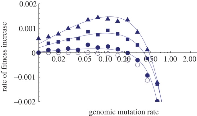
Time-averaged fitness gradients from simulations of adapting populations as a function of genomic mutation rate. Simulations are fully stochastic and individual-based; populations are asexual. (See the electronic supplementary material for details.) Each point represents the average of eight independent simulation runs. The fraction of mutations that are deleterious is constant at 0.1, and the effects of all mutations are drawn at random from an exponential distribution with mean 0.03. At high enough mutation rates, the rate of fitness increase becomes negative (indicating persistent fitness decline), from which inference of eventual extinction seems reasonable. Filled circles plot simulation results in which population size is 10 000 and the fraction of mutations that are beneficial is 10−5; filled squares plot simulation results in which population size is 50 000 and the fraction of mutations that are beneficial is 10−5; filled triangles plot simulation results in which population size is 10 000 and the fraction of mutations that are beneficial is 10−4; open circles plot simulation results in which population size is 10 000 and the fraction of mutations that are beneficial is zero (classical Muller's ratchet). (Online version in colour.)
Figure 2.

(a) Time-averaged adaptation rate as a function of genomic mutation rate. The point at which adaptation rate becomes negative marks the threshold mutation rate, indicated by the blue vertical line. (b) Predictions for the threshold mutation rate. Green triangles plot the variance threshold given by equation (2.1); blue diamonds plot the error threshold given by equation (2.4); red line plots genomic mutation rate U. Where threshold predictions intersect with the red line marks the predicted threshold mutation rate for these simulations, and coincides exactly with the observed threshold mutation rate in (a). Each point represents an average taken over the full time course of eight fully stochastic, individual-based simulations of evolving asexual populations. Population size was 10 000, fractions of mutations that were beneficial and deleterious were 0.001 and 0.5, respectively. Ten per cent of deleterious mutations were lethal; otherwise, beneficial and deleterious mutations were drawn from an exponential distribution with mean 0.03. Epistasis among deleterious mutations is synergistic with epistasis parameter 0.1 and epistasis exponent 5 (see the electronic supplementary material for epistasis function). Several similar plots with different sets of biological complexities are posted in the electronic supplementary material.
1.2.2. Neutralizing natural selection
Evolution by natural selection proceeds through the appearance and subsequent fixation of adaptive and/or compensatory mutations. When mutation rate is low, virtually all adaptive and/or compensatory mutations produced have fixation potential: all of them have the possibility, at least, of enduring the first few generations of random sampling (surviving genetic drift [50]), outcompeting other adaptive and/or compensatory mutations (surviving the Hill–Robertson effect [51] or clonal interference [52]) and spreading to fixation. This is because, with low mutation rates, progress to fixation is relatively unhindered by deleterious mutations.
As mutation rate increases, however, the fixation potential of adaptive and/or compensatory mutations is reduced: each such mutation founds a lineage whose growth is increasingly eroded by the accumulation of deleterious mutations. As mutation rate continues to increase, a point may be reached at which adaptive and/or compensatory mutations lose their fixation potential altogether, thereby neutralizing natural selection. We explore three particularly telling indicators that this point has been reached: (i) the fittest genotype in the population (e.g. an adaptive mutant) decreases in frequency, (ii) the fittest genotype in the population has an equilibrium frequency (i.e. a mutation–selection balance frequency) very close to zero, and (iii) a newly arising fittest genotype is ultimately doomed to extinction with probability one.
1.2.3. A key innovation: dynamical insufficiency
In many of the previous investigations of mutational degradation processes, analogies are drawn to physical processes not least of which is the phase transition analogy. However, the analogous physical processes typically occur on short time scales during which the relevant parameters remain constant and convergence to equilibria occurs rapidly. This context affords the luxury of dynamically sufficient models and applicability of their steady-state analyses. In evolutionary biology, however, time scales are longer, relevant parameters cannot reliably be assumed to remain constant, and equilibria may rarely, if ever, be achieved. In the face of such long-term uncertainty, predictive accuracy seems unlikely; nevertheless, dynamically insufficient models may provide short-term predictive accuracy. Fisher's ‘fundamental theorem of natural selection’ accurately predicts the evolution of fitness over the course of a single generation; by sacrificing dynamical sufficiency, this theorem achieves short-term predictive accuracy. Some of the conditions that we derive here (the more useful conditions) use variations of this approach; they depend on statistical properties of the population that, by virtue of their intermediate dynamical sufficiency, absorb contingencies and other surprises that are so characteristic of the biological world (see §3) and thereby may subsume many previous results that individually treat an array of different complexities and were derived under the purview of dynamical sufficiency.
1.2.4. Extinction
We stress that the work we present here only delineates conditions under which adaptive evolution or natural selection is neutralized. Demographic decline is not explicitly accounted for in our modelling here, and the few references we make to extinction (one of which is in §1.2.5) are therefore based on reasonable but nonetheless speculative inference. (We note that reference is made in §2.3.2 (criterion 2) to the extinction of individual beneficial lineages owing to differential or ‘relative’ fitness. This is very different from, and should not be confused with, whole-population extinction.)
1.2.5. Our default application
The discovery and development of the error threshold sparked the imagination of virologists, whose efforts to clear viral infections using antiviral drugs are bedevilled by the high mutation rates of many viruses. If mutation rate could be elevated even further through mutagenesis, then error threshold theory suggested that viral populations should undergo ‘informational collapse’, which has a dire ring to it, and suggested that populations might be driven extinct, thereby in a sense beating the virus at its own game [53–57]. As in our models, extinction in these earlier models is not explicit but may be considered a reasonable, if speculative, prediction (see §1.2.4). Partly because of this historical context, we have adopted this particular application as our ‘default’ application: unless otherwise stated, we have in mind the general aim of neutralizing adaptive evolution and/or natural selection in an unwanted population (and by extrapolation, eradicating the unwanted population) through mutagenesis, and the inequalities we derive reflect this aim.
1.2.6. Outline of this study
In this study, we independently apply the two earlier-described criteria to a standard, general model of fitness evolution in order to derive the conditions under which adaptive evolution and natural selection are neutralized. (To guide the reader, we would point out that our main results are thus indicated by the word ‘condition’.) The conditions that we derive from criterion 1 range from sufficient to sufficient and necessary; however, it is the intermediate condition—called ‘sufficient and somewhat necessary’—that we believe is the most novel and perhaps the most practical. We apply criterion 2 both to a population in which the fittest genotype is resident (recovering the classical error threshold results in a new guise that lends itself to an alternative and perhaps more useful interpretation) and to one in which the fittest genotype is a newly arising beneficial mutant.
2. Results
2.1. The model
We use a standard model of adaptive evolution of an asexual population in which a genotype or class increases in log-frequency as the fitness of that genotype or class minus the mean fitness of the population. Mutation occurs among genotypes or classes as a diffusion process that is strongly biased in favour of deleterious mutations. Mathematical formulations of this model are given in appendix A.
In what follows, we use the bracket notation in addition to the overbar notation to
denote averaging. Overbar notation is used to denote averaging over individuals in a
population. (Because our analyses implicitly assume infinite population size, such
averaging is equivalent to expectation.) Some examples are: x
denotes fitness, and  denotes the mean fitness of a population;
δx denotes the effect of
mutation on fitness, and
denotes the mean fitness of a population;
δx denotes the effect of
mutation on fitness, and  denotes its average taken over all possible mutated offspring
(here, the ‘population’ is really a potential
population). Bracket notation is used to denote averaging over time; for example,
denotes its average taken over all possible mutated offspring
(here, the ‘population’ is really a potential
population). Bracket notation is used to denote averaging over time; for example,
 denotes the mean fitness of a
population averaged over time. The models we use are continuous in time and thus our
measure of fitness x corresponds to the log of fitness
w used in classical population genetics (discrete-time)
models.
denotes the mean fitness of a
population averaged over time. The models we use are continuous in time and thus our
measure of fitness x corresponds to the log of fitness
w used in classical population genetics (discrete-time)
models.
2.2. Criterion 1: adaptive evolution is neutralized
Here, we use a formulation of our model that is continuous in both time and fitness. We ask under what conditions adaptation will move backwards, i.e. under what conditions population mean fitness will decrease in spite of an inexhaustible supply of beneficial mutations.
Assumptions of our model under this criterion are minimal: (i) no assumptions are made about the fitness landscape (except for the very weak assumption of ‘compact support’ of the mutation kernel; see appendix A), (ii) no equilibrium assumptions are made, and (iii) our results here share the tautological flavour of Fisher's theorem [58–60] (and the Price equation [61,62]) and in this sense are more akin to the theory of natural selection than to any particular model of evolution.
2.2.1. Sufficient and sufficient/necessary conditions
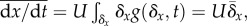
Adaptive evolution is neutralized when the long-term tendency of absolute fitness
is to decrease, despite the availability of adaptive and/or compensatory
mutations. A sufficient but not necessary version of this condition imposes
 at all times, where
 is population mean fitness.
The necessary and sufficient version of this condition is
is population mean fitness.
The necessary and sufficient version of this condition is
 . These conditions imply
(appendix A) that adaptive evolution will be neutralized and fitness will in fact
decline if the relation
. These conditions imply
(appendix A) that adaptive evolution will be neutralized and fitness will in fact
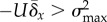
decline if the relation
| 2.1 |
holds persistently (sufficient)
or at least on average (sufficient and necessary), where
σx2 is variance in fitness, U is genomic
mutation rate and  is the average effect of mutation on fitness. (While this
expression is given in terms of fitness, an equivalent expression is derived in
terms of a fitness-related phenotype in the electronic supplementary material.) If
the effects of beneficial and deleterious mutations are considered separately,
then
is the average effect of mutation on fitness. (While this
expression is given in terms of fitness, an equivalent expression is derived in
terms of a fitness-related phenotype in the electronic supplementary material.) If
the effects of beneficial and deleterious mutations are considered separately,
then 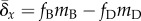 , where
fD and fB are the
fractions of all mutations that are deleterious and beneficial, respectively;
mD and mB are the mean
effects of deleterious and beneficial mutations on fitness, respectively.
Biological considerations overwhelmingly support
, where
fD and fB are the
fractions of all mutations that are deleterious and beneficial, respectively;
mD and mB are the mean
effects of deleterious and beneficial mutations on fitness, respectively.
Biological considerations overwhelmingly support 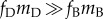 , so the left-hand side of (2.1) will most likely be
positive. By some estimates [63–68],
fB can be surprisingly high; however (i) this does
not necessarily imply high values of
fBmB [65] and (ii) it seems unlikely
that fBmB would ever
exceed fDmD, simply
because the ways to damage a highly complex entity (such as a living organism) far
outnumber the ways to improve it. In the very unlikely case that
fBmB >
fDmD, condition (2.1)
would present a contradiction, and fitness decline would be impossible regardless
of U. The accuracy of (2.1) and its robustness to several factors
such as epistasis are illustrated by figure 2 and in the electronic supplementary material.
, so the left-hand side of (2.1) will most likely be
positive. By some estimates [63–68],
fB can be surprisingly high; however (i) this does
not necessarily imply high values of
fBmB [65] and (ii) it seems unlikely
that fBmB would ever
exceed fDmD, simply
because the ways to damage a highly complex entity (such as a living organism) far
outnumber the ways to improve it. In the very unlikely case that
fBmB >
fDmD, condition (2.1)
would present a contradiction, and fitness decline would be impossible regardless
of U. The accuracy of (2.1) and its robustness to several factors
such as epistasis are illustrated by figure 2 and in the electronic supplementary material.
Critical mutation rate can be a moving target. As evidenced by
(2.1), the critical mutation rate required to neutralize adaptive evolution is a
function of the fitness variance. Increasing the mutation rate, however, will
often cause a subsequent increase in fitness variance, in turn increasing the
mutation rate required to satisfy (2.1). In fact, classical population genetics
(accounting for deleterious mutations only), and work by Rouzine et
al. [69,70] and Goyal et
al. [49]
(accounting for beneficial and deleterious mutations) all indicate that, for low
to moderate mutation rates, the fitness variance should tend towards
 following a perturbation in
fitness and/or mutation rate. This suggests that an adjustment in the mutation
rate (perhaps through increasing the dose of a mutagen, for example) to satisfy
the condition
following a perturbation in
fitness and/or mutation rate. This suggests that an adjustment in the mutation
rate (perhaps through increasing the dose of a mutagen, for example) to satisfy
the condition  will be followed by an increase in fitness variance such
that
will be followed by an increase in fitness variance such
that  , thus necessitating a
further increase in U in order to maintain the relation
, thus necessitating a
further increase in U in order to maintain the relation
 . Frank & Slatkin
[71] have pointed out that
the tendency
. Frank & Slatkin
[71] have pointed out that
the tendency  represents mutation–selection balance (in fact, they
mention this in the context of phenotypic evolution but the same notion applies).
Figuratively, the condition
represents mutation–selection balance (in fact, they
mention this in the context of phenotypic evolution but the same notion applies).
Figuratively, the condition  may be thought of as a mutation rate that persistently tips
the balance in favour of mutation; alternatively, it may be thought of as a
mutation rate persistently high enough to prevent convergence to
mutation–selection balance. As U is increased to maintain
may be thought of as a mutation rate that persistently tips
the balance in favour of mutation; alternatively, it may be thought of as a
mutation rate persistently high enough to prevent convergence to
mutation–selection balance. As U is increased to maintain
 in a continually adapting
population, σx2 will eventually reach a
maximal value (owing to finite population size) and, at this point, the value of
U need not increase further to satisfy
in a continually adapting
population, σx2 will eventually reach a
maximal value (owing to finite population size) and, at this point, the value of
U need not increase further to satisfy
 . In figure 3b, the genetic variance in
fitness is measured in simulated populations every 100 generations, and
. In figure 3b, the genetic variance in
fitness is measured in simulated populations every 100 generations, and
 is set at 10 per cent above
σx2, thereby maintaining
is set at 10 per cent above
σx2, thereby maintaining  . For a long time, the positive feedback between mutation
rate and fitness variance results in escalating adjustments to the mutation rate;
after some time, however, the variance appears to achieve a maximum, so that the
mutation rate required for continued fitness decline levels off.
. For a long time, the positive feedback between mutation
rate and fitness variance results in escalating adjustments to the mutation rate;
after some time, however, the variance appears to achieve a maximum, so that the
mutation rate required for continued fitness decline levels off.
Figure 3.

Real-time application of the different thresholds. Each panel plots a
single representative simulation run. Simulations and parameters are the
same as those in figure
1, with beneficial fraction set at 10−4.
(a,b) Variance threshold given by
equation (2.1). Every 100 generations, fitness variance is measured and
U is set equal to  (a) and
  (b). (c,d) Variance-projection
threshold given by equation (2.2). Every 500 generations, fitness
measurements are used to compute cumulants
κi(τ)
from which the
κ2(τ) are
calculated (appendix A), and U is set equal to
(b). (c,d) Variance-projection
threshold given by equation (2.2). Every 500 generations, fitness
measurements are used to compute cumulants
κi(τ)
from which the
κ2(τ) are
calculated (appendix A), and U is set equal to
 (c) and
  (d). (e,f) Error threshold given by
equation (2.4). Every 100 generations, U is set equal to
(d). (e,f) Error threshold given by
equation (2.4). Every 100 generations, U is set equal to
 (e) and
  (f). Our criterion 1 appears to perform better for
such real-time application than criterion 2.
(f). Our criterion 1 appears to perform better for
such real-time application than criterion 2.
2.2.2. Sufficient and somewhat necessary condition
So far, we have derived conditions that lie at opposite ends of the spectrum from sufficiency to sufficiency-and-necessity. From a practical standpoint, however, both are of limited utility. Condition (2.1) ensures declining fitness only for the current generation. The sufficient condition is that this relation hold persistently, but this condition may be frustratingly elusive because it fails to anticipate the change in fitness variance that typically follows an adjustment to the mutation rate. For this condition to be enforced in practice, therefore, frequent measurements of σx2 would be required, followed by adjustments in U (e.g. by increasing the dose of a mutagen), if needed, to maintain the relation (2.1) (as in figure 3a,b). In practice, therefore, the sufficient condition amounts to a rather inconvenient protocol. The sufficient-and-necessary condition, that (2.1) holds on average, requires long-term future knowledge of population fitness that is generally not attainable in practice. Here, we derive conditions that lie somewhere in the middle of the spectrum from sufficiency to sufficiency-and-necessity and that have increased practical applicability.
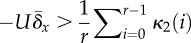
To this end, we temper our sufficient and necessary condition: instead of
requiring that the long-term average gradient oppose selection,
we now require only that the medium-term average gradient oppose
selection. We will denote this intermediate condition as
 , where r
denotes the number of future generations over which to take the average. In order
to enforce this condition, however, one needs a way to predict the near-future
course of evolution; an algorithm for doing this is outlined in Gerrish &
Sniegowski [72]. There, it is
shown that prediction of the near-future course of evolution can be achieved by a
time-discretization of a hierarchy of cumulant equations.
, where r
denotes the number of future generations over which to take the average. In order
to enforce this condition, however, one needs a way to predict the near-future
course of evolution; an algorithm for doing this is outlined in Gerrish &
Sniegowski [72]. There, it is
shown that prediction of the near-future course of evolution can be achieved by a
time-discretization of a hierarchy of cumulant equations.
Using the equations for fitness evolution derived in Gerrish & Sniegowski
[72] and imposing
 , the condition under which
adaptive evolution is neutralized may be written as
, the condition under which
adaptive evolution is neutralized may be written as
 |
2.2 |
where the future fitness
variances (or second cumulants),
κ2(τ) =
σx2(τ), are computed from the set
of recursions
κi(τ
+ 1) =
κi(τ)
+ κi
+1(τ) +
Umi as outlined in Gerrish & Sniegowski
[72] (also, see appendix A);
κi(τ)
denotes the ith cumulant at generation τ;
τ = 0 denotes the present generation (called
‘now’), τ = 1 denotes one generation
from now, τ = 2 denotes two generations from now,
etc.; and r is the ‘predictive reach’, i.e.
r is how many generations into the future the algorithm in
Gerrish & Sniegowski [72] can be trusted to predict. In ongoing work, we have shown that this
algorithm can be trusted to predict  over at least r = 20 generations in
laboratory Escherichia coli populations, and roughly
r = 45 generations in simulations [72]. An alternative condition that
errs conservatively is:
over at least r = 20 generations in
laboratory Escherichia coli populations, and roughly
r = 45 generations in simulations [72]. An alternative condition that
errs conservatively is:  . (See the electronic supplementary material for equivalent
phenotypic expressions.) The appearance of these equations is deceptively simple
because as U is changed, the predictions for
κ2(τ) will change,
i.e. the equations look explicit when in fact they are implicit for
U. (They are implicit for U because a certain
degree of circularity is required by their intermediate dynamical sufficiency,
which anticipates future changes in σx2 without requiring
knowledge of organismal and environmental parameters; in practice, this fact only
imposes the slight inconvenience of having to use an iterative procedure in the
calculations.)
. (See the electronic supplementary material for equivalent
phenotypic expressions.) The appearance of these equations is deceptively simple
because as U is changed, the predictions for
κ2(τ) will change,
i.e. the equations look explicit when in fact they are implicit for
U. (They are implicit for U because a certain
degree of circularity is required by their intermediate dynamical sufficiency,
which anticipates future changes in σx2 without requiring
knowledge of organismal and environmental parameters; in practice, this fact only
imposes the slight inconvenience of having to use an iterative procedure in the
calculations.)
2.3. Criterion 2: natural selection is neutralized
The approach that derives from this criterion takes its lead from statistical physics, where an ‘order parameter’ quantifies the degree of order present in the system at hand. Order in an evolving population is brought about through the action of natural selection on genetic variation. In evolution, a natural choice for an order parameter is the frequency of the fittest genotype. If natural selection is operational, the fittest genotype should persist at reasonable frequency despite recurrent mutation away from this genotype, and this frequency is thus indicative of the amount of order present in the population. As mutation rate increases, the frequency of the fittest genotype will decrease, indicating a decrease in the overall order present. At a sufficiently high mutation rate, the amount of order will approach zero.
Assumptions implicit under this condition again are minimal: (i) no assumptions are made about the fitness landscape (e.g. the ‘single-peak’ landscape used by many error-threshold models is not required here; curiously, Eigen's original paper on the error threshold had a formulation similar to ours—as shown in §3—and also did not require a ‘single-peak’ landscape) and (ii) equilibrium is not assumed, although some of the results are obtained by solving for the equilibrium state.
2.3.1. Sufficient condition
Here, we have in mind a population that is heterogeneous and that is predominated by a fittest genotype whose frequency is u0. Our sufficient condition is derived by finding the mutation rate that causes the frequency of the fittest genotype to decrease relative to its mutational neighbours: du0/dt < 0, persistently. Solving for the mutation rate that ensures this inequality gives rise to the condition
| 2.3 |
where L is the
size of the deleterious genome, x0 is the fitness of
the fittest genotype;  , and
, and  , from which we have the useful relation
 . In a finite population,
x0 is the maximum fitness found in the population,
and
. In a finite population,
x0 is the maximum fitness found in the population,
and  is the average fitness of
everybody else:
is the average fitness of
everybody else:  , where S is the subset of the population
that has fitness less than the maximum and #S is the
number of individuals in that subset. If it is the case that the population is
finite and
, where S is the subset of the population
that has fitness less than the maximum and #S is the
number of individuals in that subset. If it is the case that the population is
finite and  , then the term
  , giving rise to the condition:

 (reported in table 1). In our simulations, we assume an infinite genome (L
→ ∞) and finite population size; under these conditions,
(reported in table 1). In our simulations, we assume an infinite genome (L
→ ∞) and finite population size; under these conditions,
 is exact. In a continually
adapting population,
is exact. In a continually
adapting population,  will be small most of the time, in which case this
expression may be used interchangeably with:
will be small most of the time, in which case this
expression may be used interchangeably with: 
 (used in figure
3).
(used in figure
3).
Table 1.
Summary of neutralizing conditions.
| conditions | adaptive evolution (criterion 1) | natural selection (criterion 2) |
|---|---|---|
| sufficient |
 persistently
 |
  persistentlya
|
| sufficient and somewhat necessary |
 intermittently
 |
|
| sufficient and necessary |
 long-term
average long-term
average |
 long-term
steady state long-term
steady state |
aThis condition holds when  .
.
2.3.2. Sufficient and necessary conditions
(1) Mutational degradation of an established fittest genotype.
Here, we have in mind a population that is heterogeneous but that has been
predominated by a fittest lineage for some time. To determine the amount of order
in this population, we compute its order parameter,
 : the equilibrium frequency
of this fittest lineage relative to its mutational neighbours (genotypes that
differ from the fittest lineage by mutation). We are especially interested in what
happens to the order parameter as mutation rate increases.
: the equilibrium frequency
of this fittest lineage relative to its mutational neighbours (genotypes that
differ from the fittest lineage by mutation). We are especially interested in what
happens to the order parameter as mutation rate increases.
Analysis of the evolutionary model at equilibrium reveals that, indeed, the order
parameter  decreases with increasing mutation rate (appendix A). The
approach of
decreases with increasing mutation rate (appendix A). The
approach of  towards zero as U increases is
characterized by an inflection point that becomes increasingly sharp as
deleterious genome size L increases. The mutation rate at which
the inflection point occurs is found by solving for the critical mutation rate
Uc that satisfies
towards zero as U increases is
characterized by an inflection point that becomes increasingly sharp as
deleterious genome size L increases. The mutation rate at which
the inflection point occurs is found by solving for the critical mutation rate
Uc that satisfies  . As L increases,
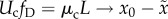 , where
fD is again the fraction of mutations that are
deleterious, and μc is the critical point
mutation rate. From this result, natural selection may reasonably be expected to
be neutralized when mutation exceeds the critical rate:
, where
fD is again the fraction of mutations that are
deleterious, and μc is the critical point
mutation rate. From this result, natural selection may reasonably be expected to
be neutralized when mutation exceeds the critical rate:
| 2.4 |
This is the classical ‘error threshold’ result in new guise. It is an equilibrium result and its practical use would therefore require knowledge of long-term future states of the population. When long-term data are available this condition is very accurate and is robust to many factors (figure 2 and electronic supplementary material).
The equilibrium frequency of the fittest class or genotype at the ‘error
threshold’, while greatly reduced, is still greater than the frequencies of
neighbouring genotypes: at μ =
μc, the fittest genotype has frequency
 , whereas mutational
neighbours have frequency
, whereas mutational
neighbours have frequency  . This stands in contrast to common notions about the error
threshold as creating a competitive reversal that leads to the subordination
and/or loss of the fittest genotype. In a finite population, the fittest genotype
will be deterministically lost from the population at the error threshold only if
. This stands in contrast to common notions about the error
threshold as creating a competitive reversal that leads to the subordination
and/or loss of the fittest genotype. In a finite population, the fittest genotype
will be deterministically lost from the population at the error threshold only if

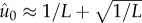
 . To put this condition in perspective, we consider a strain
of Escherichia coli that has a genome of length
. To put this condition in perspective, we consider a strain
of Escherichia coli that has a genome of length
 base pairs; if we make the
very conservative assumption that mutation at any position on the genome will
affect fitness, then any population larger than
base pairs; if we make the
very conservative assumption that mutation at any position on the genome will
affect fitness, then any population larger than  will deterministically retain the fittest genotype at the
error threshold.
will deterministically retain the fittest genotype at the
error threshold.
Despite the persistence and continued dominance of the fittest genotype, the error
threshold nevertheless marks a point at which the frequencies of the different
genotypes are so severely eroded by mutation that their frequencies are clearly
not indicative of their fitness. This neutralizing of natural selection is
apparent in the relation: 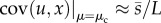 , where
  . For large genomes, therefore, the covariance between
fitness and frequency—an indicator of the efficacy of natural
selection—is very small at the error threshold (but still positive).
Additionally, the extent to which natural selection has become ineffective is
reflected by the amount of disorder present in the equilibrium
population; a standard index of disorder is the Shannon entropy (measured, for
example, for RNA viral quasi-species [34]) which, at the error threshold, is approximately equal to
log2L.
. For large genomes, therefore, the covariance between
fitness and frequency—an indicator of the efficacy of natural
selection—is very small at the error threshold (but still positive).
Additionally, the extent to which natural selection has become ineffective is
reflected by the amount of disorder present in the equilibrium
population; a standard index of disorder is the Shannon entropy (measured, for
example, for RNA viral quasi-species [34]) which, at the error threshold, is approximately equal to
log2L.
(2) Mutational degradation of a newly arising fittest genotype.
Here, we have in mind an asexual population that is heterogeneous and in which a
beneficial mutation emerges. This mutation creates a newly arising ‘fittest
genotype’ whose subsequent growth depends on the persistence of that
genotype within the growing lineage, despite recurrent mutation away from that
genotype. The newly arising fittest genotype has fitness
x0, and the rest of the population has average
fitness  , as before. In a single
generation, the new lineage grows by a factor
, as before. In a single
generation, the new lineage grows by a factor  . Accumulation of deleterious mutations occurs most rapidly
early in the growth of a lineage [9], when
. Accumulation of deleterious mutations occurs most rapidly
early in the growth of a lineage [9], when  , suggesting the approximation
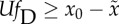
 . Previous studies show that
genomic mutation rates that cause the degradation of the newly arising fittest
genotype must satisfy UfD ≥
logR [9,73,74]. The extinction of a newly
arising fittest genotype is therefore predicted to occur when
. Previous studies show that
genomic mutation rates that cause the degradation of the newly arising fittest
genotype must satisfy UfD ≥
logR [9,73,74]. The extinction of a newly
arising fittest genotype is therefore predicted to occur when
| 2.5 |
Compare with (2.4). This result
was originally derived for an independent asexual population growing without bound
at discrete-time rate R [9] and was later re-derived in a way that more
explicitly allowed for purifying selection and dubbed the ‘lethal
mutagenesis’ threshold [73,74] for
unboundedly growing viral and bacterial populations. This result should also
apply, however, to lineages growing within a population as a consequence of
positive relative fitness  . Finite population size restricts applicability to lineages
that begin to decline in frequency before being affected by population size
constraints, which seems likely to account for many such lineages when at or near
the critical mutation rate (but see Gerrish et al. [75]). Those lineages that do
achieve higher frequencies are likely to become fixed in the population, in which
case the relevant condition was derived in the previous subsection:
. Finite population size restricts applicability to lineages
that begin to decline in frequency before being affected by population size
constraints, which seems likely to account for many such lineages when at or near
the critical mutation rate (but see Gerrish et al. [75]). Those lineages that do
achieve higher frequencies are likely to become fixed in the population, in which
case the relevant condition was derived in the previous subsection:
 (condition (2.4)). It thus
seems reasonable to conjecture that whatever the maximum frequency achieved by the
new lineage, the condition is well approximated by (2.5).
(condition (2.4)). It thus
seems reasonable to conjecture that whatever the maximum frequency achieved by the
new lineage, the condition is well approximated by (2.5).
3. Discussion
3.1. Practical use of the equations
3.1.1. Why are accurate predictions desirable?
On the surface, it seems that if one has the ability to increase mutation rate, perhaps through the use of a chemical mutagen, then to drive a population extinct, one needs only to increase the mutation rate by a large amount, perhaps by administering a high dose of mutagen. The problem with this approach is that, in real populations, variation in mutation rate is inevitable, and resistance to a mutagen can appear. A large increase in the mutation rate can create strong selection pressure for a lowered mutation rate, and a reduction in the mutation rate may thus evolve in short order. Our own work with a mutator strain of Escherichia coli and a nucleoside analogue mutagen, together with several previous mutagenesis studies using different viral systems, shows that resistance to mutagens at high doses can evolve rapidly and through a number of different mechanisms [76–82]. If one could increase the mutation rate to a level that is high enough to cause extinction, but not too high, selection for resistance could, in principle, be reduced considerably and the evolution of resistance might be prevented. Accurate predictions for the critical mutation rate required for extinction may therefore aid in the practical implementation of chemical mutagenesis, and the evolution of resistance might be prevented. Indeed, our equations and simulations would suggest an improved protocol in which a mutagen is administered in incrementally increasing dose (reflected in figure 3).
3.1.2. Timeframe of applicability
The equations derived here are similar in their generality and robustness; however, they differ among themselves in one aspect of practical relevance, namely, their timeframe of applicability. Under criterion 1, this timeframe ranges from short-term (sufficient) to medium-term (sufficient and somewhat necessary) to long-term (sufficient and necessary). Under criterion 2, the timeframe is short-term (sufficient) or long-term (sufficient and necessary). The long-term results might potentially be applied approximately using a running-average approach that is necessarily somewhat arbitrary, but technically correct application of these results requires information about long-term future states of the population that would not be obtainable in practice. When the mutation rate is adjusted according to fitness measurements from a population taken in real time, the correct equations to use are the short-term and medium-term conditions. These conditions are applied in simulation studies of which representative runs are presented in figure 3; there, adjustments to the mutation rate are made in real time, and the short-term and medium-term conditions derived under criterion 1 (labelled ‘variance’ and ‘variance-projection’ thresholds, respectively) perform well, whereas the conditions derived under criterion 2 (error threshold) appear to be less well suited to such real-time application.
3.1.3. Adaptation in a static environment
A population adapting in a static environment typically has a limited,
non-renewable supply of available beneficial mutations (barring intransitive
interactions). As the population adapts, therefore, the supply of available
beneficial mutations is slowly depleted; as a consequence, mean fitness may
increase and subsequently decrease, and fitness variance may also change over
time, thereby changing the minimal mutation rate prescribed by criterion 1. In
particular, as a population adapts to a static environment, fitness variance
should decrease, thereby decreasing the predicted threshold
mutation rate. Eventually, the threshold mutation rate may decrease to a value
that is below the population mutation rate such that further adaptive evolution is
neutralized. This is shown schematically in figure 4: in static environments and, generally
speaking, in environments where the supply of beneficial mutations can change over
time, adaptive evolution or natural selection may be neutralized not as a result
of changes in the mutation rate (i.e. changes in U) but as a
result of changes in the requirements on the mutation rate (i.e. changes in
 and in
 ).
).
Figure 4.

Schematic of how adaptive evolution and/or natural selection may be neutralized not as a result of increasing the mutation rate but as a result of a decreasing threshold mutation rate. The red line indicates the mutation rate of the population; the black line plots the threshold mutation rate as a function of the fraction of mutations that are beneficial (horizontal axis). The big blue arrow indicates that as a population adapts in a static environment, its supply of beneficial mutations is used up, resulting in a decreasing fraction of mutations that are beneficial. As this fraction decreases, the threshold mutation rate decreases, until eventually the threshold mutation rate is below the mutation rate of the population.
3.2. Connections to previous theory
3.2.1. Fisher and Kimura
Fisher's ‘fundamental theorem of natural selection’ states
that, when x is defined as additive genetic fitness,
 quite generally [59,83]. Fisher's theorem shows that this
particular component of fitness can only increase (variance is a non-negative
quantity); consequently, this component of fitness has accurately been called the
‘adaptive engine’ of natural selection [60]. This component of fitness, however, must be
conserved over time, for example, in the transmission from parent to offspring for
Fisher's theorem to apply. If there is a component of fitness that is not
conserved, then to find the change in total mean fitness of the
population (conserved and non-conserved), one must use the product and chain
rules:
quite generally [59,83]. Fisher's theorem shows that this
particular component of fitness can only increase (variance is a non-negative
quantity); consequently, this component of fitness has accurately been called the
‘adaptive engine’ of natural selection [60]. This component of fitness, however, must be
conserved over time, for example, in the transmission from parent to offspring for
Fisher's theorem to apply. If there is a component of fitness that is not
conserved, then to find the change in total mean fitness of the
population (conserved and non-conserved), one must use the product and chain
rules:  which, together with
 yields
 —a fact pointed out
by Kimura [84]. (We note that
—a fact pointed out
by Kimura [84]. (We note that
 denotes the mean change in
‘individual’ fitness, where the mean is taken over individuals in
the population.) As a general rule,
denotes the mean change in
‘individual’ fitness, where the mean is taken over individuals in
the population.) As a general rule,  will be negative, because random alterations in the
organism or its environment are more likely to decrease the organism's
fitness than to increase it. This simple calculation illustrates the fact that
Fisher's fundamental theorem applies only to that subset of the population
whose additive genic fitness is conserved over the period of time in question:
only for this particular subset of the population are we guaranteed that mean
fitness will not decrease.
will be negative, because random alterations in the
organism or its environment are more likely to decrease the organism's
fitness than to increase it. This simple calculation illustrates the fact that
Fisher's fundamental theorem applies only to that subset of the population
whose additive genic fitness is conserved over the period of time in question:
only for this particular subset of the population are we guaranteed that mean
fitness will not decrease.
Applying our criterion 1 to Kimura's equation yields a more general condition for the neutralizing of adaptive evolution:
| 3.1 |
must hold persistently or at
least on average. Here, the mechanism of change in individual fitness over time is
not specified. If we specify that the mechanism of change is mutation, then
 where
where
 is the distribution of
mutational effects on fitness, and we recover equation (2.1).
is the distribution of
mutational effects on fitness, and we recover equation (2.1).
3.2.2. The error threshold
As previously stated, equations (2.4) and (2.5) are the error threshold in new
guise. The original work on the error threshold due to Eigen [16] derives a minimum value for
the ‘quality factor’—the probability of complete fidelity of
replication—that is needed to maintain the efficacy of natural selection
and thus to support life. This minimum value is given by
 (equation II-45 in Eigen
[16]), where
(equation II-45 in Eigen
[16]), where
 and
and
 are the birth and death
rates of the fittest genotype (the ‘master sequence’), respectively,
are the birth and death
rates of the fittest genotype (the ‘master sequence’), respectively,
 and
and
 are the mean birth and
death rates of the rest of the population (individuals that do not carry the
‘master sequence’). The quantity
are the mean birth and
death rates of the rest of the population (individuals that do not carry the
‘master sequence’). The quantity  is the expected number of deleterious mutants produced by a
single replication event of the fittest genotype. This quantity, in our notation,
is UfD; furthermore,
is the expected number of deleterious mutants produced by a
single replication event of the fittest genotype. This quantity, in our notation,
is UfD; furthermore,  is equivalent to our x0 and
 is equivalent to our
 . Eigen's result may
thus be rewritten in our notation as requiring
. Eigen's result may
thus be rewritten in our notation as requiring  for the effectiveness of natural selection to be
maintained, or conversely,
for the effectiveness of natural selection to be
maintained, or conversely,  for natural selection to be neutralized.
In work subsequent to Eigen's original publication, the varied
presentations of his error threshold result are usually rearrangements of this
simple expression: qminL =
σ−1, where
qmin is the minimum per-nucleotide replication
fidelity required for survival (qmin =
1−μc), L is the
length of the deleterious genome, and σ is the
‘superiority parameter’, defined as  . Rewriting reveals an interesting biological requirement:
 gives rise to the
relation
gives rise to the
relation
| 3.2 |
This inverse relation between
μc and L intrigued its
discoverers to the extent that the ‘something’ was all but ignored.
It was since discovered, however, that observations of μL
are surprisingly constant across microbial taxa [85,86] (indeed, it has been conjectured that this is the case precisely
because of the inverse relation between μc and
L). The relative constancy of μL
across taxa suggests that the ‘something’ may in fact be quite
relevant to the fate of a population; furthermore, L will
probably not change on time scales pertinent to extinction-by-mutation. These
considerations shift the focus to σ. Its name together
with its traditional presentation obfuscates the fact that
σ is a population-dependent quantity
and not an organism-dependent parameter. Our new presentation of
this old result shifts the emphasis from critical point mutation
rate μc versus genome length L
to critical genomic mutation rate
μcL versus the myriad
biological, ecological and environmental factors that are not explicitly part of
the equation but that are absorbed by the quantity σ or,
in our formulation,  .
.
3.3. Connections among results presented here
Our first criterion is the sustained decline of absolute fitness, whereas our second
criterion is the inefficacy of natural selection. We now show that, despite these
perhaps disparate criteria, the resulting conditions for extinction connect through
classical population genetics. Criterion 1 gives rise to the condition
 , and criterion 2 gives rise to
the condition
, and criterion 2 gives rise to
the condition  . Our comparison of these two results proceeds by multiplying
both sides of the second condition by mD to obtain
. Our comparison of these two results proceeds by multiplying
both sides of the second condition by mD to obtain
 . First, we note that the
left-hand side is
. First, we note that the
left-hand side is  because most mutations are deleterious. Next, we focus on the
right-hand side of the inequality. As a population approaches the error threshold
(i.e. as this inequality approaches equality), the size of the fittest class
approaches zero and it is the case that
because most mutations are deleterious. Next, we focus on the
right-hand side of the inequality. As a population approaches the error threshold
(i.e. as this inequality approaches equality), the size of the fittest class
approaches zero and it is the case that  , or
, or  . The quantity
  is known in classical population genetics as the genetic load,
and it is known to converge to the deleterious mutation rate
UfD. Furthermore, it is known that if mutations are
assumed to have a fixed deleterious effect, mD, then the
number of accumulated mutations becomes Poisson distributed with mean
UfD/mD [6]. The variance in number of
accumulated mutations is the same as the mean, and the variance in
fitness is therefore
is known in classical population genetics as the genetic load,
and it is known to converge to the deleterious mutation rate
UfD. Furthermore, it is known that if mutations are
assumed to have a fixed deleterious effect, mD, then the
number of accumulated mutations becomes Poisson distributed with mean
UfD/mD [6]. The variance in number of
accumulated mutations is the same as the mean, and the variance in
fitness is therefore  . As the error threshold is approached, therefore, the
right-hand side becomes
. As the error threshold is approached, therefore, the
right-hand side becomes  .
.
3.4. Borrowed robustness
Fisher's fundamental theorem of natural selection is known to be extraordinarily accurate in spite of numerous complexities that are characteristic of real populations. Because (2.1) is implicit in the results of Fisher and Kimura, therefore, we expect these results to be quite robust to numerous biological complexities. Furthermore, the convergence we have demonstrated between (2.1), (2.3) and (2.5) leads us to believe that the classical error threshold result is similarly robust, although it does not appear to perform as well in real time (figure 3). Figure 2 together with the plots we have posted in the electronic supplementary material—and many others not posted—demonstrate the robustness of (2.1) (and by inference (2.2)) to a wide range of complexities, including finite genome effects, the effects of finite population size (including Muller's ratchet), epistatic interactions among mutations, environmental noise (random changes in fitness caused by unspecified factors), an evolving mutational robustness modifier, compensatory mutations whose rate increases with decreasing fitness, an evolving mutation rate modifier and a fraction of mutations that are lethal.
Acknowledgements
Special thanks to Cristian Batista for insightful explanations of the error threshold as a phase transition, to Isabel Gordo for helping make connections among the different theories and to Claus Wilke for helpful comments and clarifications. We also thank Michael Lassig, Paul Joyce, Alan Perelson, Boris Shraiman, Sidhartha Goyal, Daniel Balick, Nico Stollenwerk, Gabriela Gomes, Ana Margarida Sousa, Jorge Carneiro and Josep Sardanyés for helpful discussions, and two anonymous reviewers for helpful comments. Much of this research was developed thanks to fertile environments provided by two institutes: the Kavli Institute for Theoretical Physics in Santa Barbara, CA (2011 Microbial and Viral Evolution workshop), and the Instituto Gulbenkian de Ciências in Oeiras, Portugal. This work was supported by the US National Institutes of Health. grants: R01 GM079843-01 (P.J.G./P.D.S.), R01 GM079483-02S1 (P.J.G./P.D.S.), a seed grant through 1P20RR18754 (Center for Evolutionary and Theoretical Immunology) (P.J.G.), UM1-AI100645–01 (Center for HIV/AIDS Vaccine Immunology-Immunogen Design; P.J.G.); and European Commission grant no. FP7 231807 (P.J.G.).
Appendix A
The results we describe in the main text derive from two manifestations of a standard model of evolution described verbally in §2.1. Here, we give the mathematical details of those manifestations.
A.1. Model in continuous fitness for criterion 1
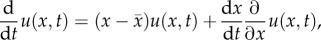
We let u(x,t) denote the density of individuals in the population with log-fitness x at time t. Mutation can create ‘jumps’ in log-fitness whose size has probability density g(ϕ, t) at time t. Under selection and mutation, a population's evolution is described by:
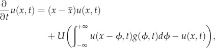 |
A1 |
where
 . If we apply the standard diffusion approximation to the
mutation term, then this equation becomes
. If we apply the standard diffusion approximation to the
mutation term, then this equation becomes
| A2 |
Mutation operator,
 , where
 and
and
 ; fB is the fraction of all
mutations that are beneficial (‘beneficial fraction’),
fD is the deleterious fraction;
mB and mD are the
mean effects of beneficial and deleterious mutations on fitness, respectively;
σB2 and σD2 are the variances in those effects. We multiply both
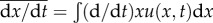
sides of (A 2) by x and integrate over all x
to obtain
; fB is the fraction of all
mutations that are beneficial (‘beneficial fraction’),
fD is the deleterious fraction;
mB and mD are the
mean effects of beneficial and deleterious mutations on fitness, respectively;
σB2 and σD2 are the variances in those effects. We multiply both
sides of (A 2) by x and integrate over all x
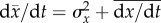
to obtain  . Under the reasonable assumption that
u(x,t) has compact
support in x, integration by parts gives
. Under the reasonable assumption that
u(x,t) has compact
support in x, integration by parts gives
 , where
  . The condition
  reflects the neutralizing of adaptive evolution and is
met when
reflects the neutralizing of adaptive evolution and is
met when  .
.
A.2. Model in discrete fitness for criterion 2
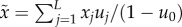
As an indication of the amount of order in the system at hand, we would like to know the frequency of the fittest genotype relative to its mutational neighbours. The dynamics of this genotype and its mutational neighbours (genotypes that differ from the fittest genotype by mutation) are given by this set of equations:
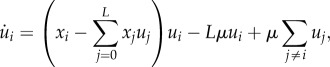 |
A3 |
where u0 is the frequency of the fittest genotype (the order parameter), ui is the frequency of mutational neighbour, i = 1, 2, 3, ..., L, xi is fitness of genotype i, and μ is point mutation rate.
The equation for the fittest genotype u0 may be written as
| A4 |
where
x0 is the fitness of the fittest genotype and
 is the average fitness of everybody else:
 . We note that
  is not relative fitness; a possible interpretation of
the value
is not relative fitness; a possible interpretation of
the value  is that it is the reproductive ‘pay-off’
in a game played by the fittest genotype against everybody else.
is that it is the reproductive ‘pay-off’
in a game played by the fittest genotype against everybody else.
A.3. Calculating the ‘sufficient and somewhat necessary’ conditions under criterion 1
To compute the ‘sufficient and somewhat necessary’ conditions requires projection of cumulants κi(τ) over a period of r generations into the future. Recurrence relations that do this are developed in Gerrish & Sniegowski [72].
The terms of the sum in (2.2) are computed from the recurrence relation:
 for all
  , where
κi(τ)
is the ith cumulant in fitness at a time
τ generations from now, U is
genomic mutation rate and mi is the
ith raw moment of the distribution of mutational effects on
fitness.
, where
κi(τ)
is the ith cumulant in fitness at a time
τ generations from now, U is
genomic mutation rate and mi is the
ith raw moment of the distribution of mutational effects on
fitness.
The practical implementation of condition (2.2) requires some care. The procedure outlined in Gerrish & Sniegowski [72] provides methods for estimating the mj. These parameters cannot be estimated separately from U; only their products Umj can be estimated, if the equations are left in non-parametric form. The obvious remedy is to make the equations parametric by writing the known expressions for the moments of an assumed distribution in place of mj. Then, the parameters to be estimated are U and the limited number of parameters of the assumed distribution, and U can then be estimated separately. If one's objective is to monitor a population's risk of extinction, or to drive a population extinct through mutagenesis, however, a less obvious remedy may apply. In such cases, absolute mutation rates may be irrelevant, and the effects of an increased (or decreased) mutation rate can be predicted by simply multiplying the estimates of Umj by the factor by which mutation rate is increased (or decreased). In such cases, therefore, the equations may be left in non-parametric form.
References
- 1.Carrasco P, de la Iglesia F, Elena SF. 2007. Distribution of fitness and virulence effects caused by single-nucleotide substitutions in tobacco etch virus. J. Virol. 81, 12 979–12 984 10.1128/JVI.00524-07 (doi:10.1128/JVI.00524-07) [DOI] [PMC free article] [PubMed] [Google Scholar]
- 2.Sanjuán R. 2010. Mutational fitness effects in RNA and single-stranded DNA viruses: common patterns revealed by site-directed mutagenesis studies. Phil. Trans. R. Soc. B 365, 1975–1982 10.1098/rstb.2010.0063 (doi:10.1098/rstb.2010.0063) [DOI] [PMC free article] [PubMed] [Google Scholar]
- 3.Sanjuán R, Moya A, Elena SF. 2004. The distribution of fitness effects caused by single-nucleotide substitutions in an RNA virus. Proc. Natl Acad. Sci. USA 101, 8396–8401 10.1073/pnas.0400146101 (doi:10.1073/pnas.0400146101) [DOI] [PMC free article] [PubMed] [Google Scholar]
- 4.Muller H. 1932. Some genetic aspects of sex. Am. Nat. 66, 118–138 10.1086/280418 (doi:10.1086/280418) [DOI] [Google Scholar]
- 5.Felsenstein J. 1974. The evolutionary advantage of recombination. Genetics 78, 737–756 [DOI] [PMC free article] [PubMed] [Google Scholar]
- 6.Haigh J. 1978. The accumulation of deleterious genes in a population: Muller's ratchet. Theor. Popul. Biol. 14, 251–267 10.1016/0040-5809(78)90027-8 (doi:10.1016/0040-5809(78)90027-8) [DOI] [PubMed] [Google Scholar]
- 7.Andersson D, Hughes D. 1996. Muller's ratchet decreases fitness of a DNA-based microbe. Proc. Natl Acad. Sci. USA 93, 906–907 10.1073/pnas.93.2.906 (doi:10.1073/pnas.93.2.906) [DOI] [PMC free article] [PubMed] [Google Scholar]
- 8.Chao L, Tran T, Matthews C. 1992. Muller's ratchet and the advantage of sex in the RNA virus 6. Evolution 46, 289–299 10.2307/2409851 (doi:10.2307/2409851) [DOI] [PubMed] [Google Scholar]
- 9.Fontanari JF, Colato A, Howard RS. 2003. Mutation accumulation in growing asexual lineages. Phys. Rev. Lett. 91, 218101. 10.1103/PhysRevLett.91.218101 (doi:10.1103/PhysRevLett.91.218101) [DOI] [PubMed] [Google Scholar]
- 10.Gordo I, Charlesworth B. 2000. On the speed of Muller's ratchet. Genetics 156, 2137–2140 [DOI] [PMC free article] [PubMed] [Google Scholar]
- 11.Green DM. 1990. Muller's Ratchet and the evolution of supernumerary chromosomes. Genome 33, 818–824 10.1139/g90-123 (doi:10.1139/g90-123) [DOI] [Google Scholar]
- 12.Heller R, Smith JM. 2009. Does Muller's ratchet work with selfing? Genet. Res. 32, 289–293 10.1017/S0016672300018784 (doi:10.1017/S0016672300018784) [DOI] [Google Scholar]
- 13.Kondrashov AS. 1984. Deleterious mutations as an evolutionary factor: 1. The advantage of recombination. Genet. Res. 44, 199–217 10.1017/S0016672300026392 (doi:10.1017/S0016672300026392) [DOI] [PubMed] [Google Scholar]
- 14.Loewe L, Lamatsch DK. 2008. Quantifying the threat of extinction from Muller's ratchet in the diploid Amazon molly (Poecilia formosa). BMC Evol. Biol. 8, 88. 10.1186/1471-2148-8-88 (doi:10.1186/1471-2148-8-88) [DOI] [PMC free article] [PubMed] [Google Scholar]
- 15.Yuste E, Sanchez-Palomino S, Casado C, Domingo E, López-Galíndez C. 1999. Drastic fitness loss in human immunodeficiency virus type 1 upon serial bottleneck events. J. Virol. 73, 2745–2751 [DOI] [PMC free article] [PubMed] [Google Scholar]
- 16.Eigen M. 1971. Self organization of matter and the evolution of biological macro-molecules. Die Naturwissenschaften 58, 465–523 10.1007/BF00623322 (doi:10.1007/BF00623322) [DOI] [PubMed] [Google Scholar]
- 17.Eigen M. 2002. Error catastrophe and antiviral strategy. Proc. Natl Acad. Sci. USA 99, 13 374–13 376 10.1073/pnas.212514799 (doi:10.1073/pnas.212514799) [DOI] [PMC free article] [PubMed] [Google Scholar]
- 18.Biebricher CK, Eigen M. 2005. The error threshold. Virus Res. 107, 117–127 10.1016/j.virusres.2004.11.002 (doi:10.1016/j.virusres.2004.11.002) [DOI] [PubMed] [Google Scholar]
- 19.Biebricher CK, Eigen M. 2006. What is a quasispecies? Curr. Top. Microbiol. Immunol. 299, 1–31 10.1007/3-540-26397-7_1 (doi:10.1007/3-540-26397-7_1) [DOI] [PubMed] [Google Scholar]
- 20.Eigen M. 2000. Natural selection: a phase transition? Biophys. Chem. 85, 101–123 10.1016/S0301-4622(00)00122-8 (doi:10.1016/S0301-4622(00)00122-8) [DOI] [PubMed] [Google Scholar]
- 21.Wolff A, Krug J. 2009. Robustness and epistasis in mutation–selection models. Phys. Biol. 6, 036007. 10.1088/1478-3975/6/3/036007 (doi:10.1088/1478-3975/6/3/036007) [DOI] [PubMed] [Google Scholar]
- 22.Hermisson J, Redner O, Wagner H, Baake E. 2002. Mutation–selection balance: ancestry, load, and maximum principle. Theor. Popul. Biol. 62, 9–46 10.1006/tpbi.2002.1582 (doi:10.1006/tpbi.2002.1582) [DOI] [PubMed] [Google Scholar]
- 23.Tarazona P. 1992. Error thresholds for molecular quasispecies as phase transitions: from simple landscapes to spin-glass models. Phys. Rev. A 45, 6038–6050 10.1103/PhysRevA.45.6038 (doi:10.1103/PhysRevA.45.6038) [DOI] [PubMed] [Google Scholar]
- 24.Summers J, Litwin S. 2006. Examining the theory of error catastrophe. J. Virol. 80, 20–26 10.1128/JVI.80.1.20-26.2006 (doi:10.1128/JVI.80.1.20-26.2006) [DOI] [PMC free article] [PubMed] [Google Scholar]
- 25.Boerlijst MC, Bonhoeffer S, Nowak MA. 1996. Viral quasi-species and recombination. Proc. R. Soc. Biol. Sci. 263, 1577–1584 10.1098/rspb.1996.0231 (doi:10.1098/rspb.1996.0231) [DOI] [Google Scholar]
- 26.Nilsson M, Snoad N. 2000. Error thresholds for quasispecies on dynamic fitness landscapes. Phys. Rev. Lett. 84, 191–194 10.1103/PhysRevLett.84.191 (doi:10.1103/PhysRevLett.84.191) [DOI] [PubMed] [Google Scholar]
- 27.Ochoa G, Harvey I. 1999. Recombination and error thresholds in finite populations. In Foundations of genetic algorithms 5 (eds Banzhaf W, Reeves C.), pp. 245–264 San Francisco, CA: Morgan Kaufmann Publishers, Inc [Google Scholar]
- 28.Sardanyés J, Elena SF. 2010. Error threshold in RNA quasispecies models with complementation. J. Theor. Biol. 265, 278–286 10.1016/j.jtbi.2010.05.018 (doi:10.1016/j.jtbi.2010.05.018) [DOI] [PubMed] [Google Scholar]
- 29.Elena SF, Solé RV, Sardanyés J. 2010. Simple genomes, complex interactions: epistasis in RNA virus. Chaos 20, 026106. 10.1063/1.3449300 (doi:10.1063/1.3449300) [DOI] [PubMed] [Google Scholar]
- 30.Sardanyés J, Elena SF. 2011. Quasispecies spatial models for RNA viruses with different replication modes and infection strategies. PLoS ONE 6, e24884. 10.1371/journal.pone.0024884 (doi:10.1371/journal.pone.0024884) [DOI] [PMC free article] [PubMed] [Google Scholar]
- 31.Sardanyés J, Martínez F, Daròs J-A, Elena SF. 2012. Dynamics of alternative modes of RNA replication for positive-sense RNA viruses. J. R. Soc. Interface 9, 768–776 10.1098/rsif.2011.0471 (doi:10.1098/rsif.2011.0471) [DOI] [PMC free article] [PubMed] [Google Scholar]
- 32.Sardanyés J, Solé RV. 2006. Bifurcations and phase transitions in spatially extended two-member hypercycles. J. Theor. Biol. 243, 468–482 10.1016/j.jtbi.2006.07.014 (doi:10.1016/j.jtbi.2006.07.014) [DOI] [PubMed] [Google Scholar]
- 33.Sardanyes J, Sole RV, Elena SF. 2009. Replication mode and landscape topology differentially affect RNA virus mutational load and robustness. J. Virol. 83, 12 579–12 589 10.1128/JVI.00767-09 (doi:10.1128/JVI.00767-09) [DOI] [PMC free article] [PubMed] [Google Scholar]
- 34.Solé R, Sardanyes J, Diez J, Mas A. 2006. Information catastrophe in RNA viruses through replication thresholds. J. Theor. Biol. 240, 353–359 10.1016/j.jtbi.2005.09.024 (doi:10.1016/j.jtbi.2005.09.024) [DOI] [PubMed] [Google Scholar]
- 35.Bonhoeffer S, Stadler P. 1993. Error thresholds on correlated fitness landscapes. J. Theor. Biol. 164, 359–372 10.1006/jtbi.1993.1160 (doi:10.1006/jtbi.1993.1160) [DOI] [Google Scholar]
- 36.Gerrish PJ. 2009. Some observations about the nearest-neighbor model of the error threshold. AIP Conf. Proc. 1168, 1564–1568 10.1063/1.3241401 (doi:10.1063/1.3241401) [DOI] [Google Scholar]
- 37.Takeuchi N, Hogeweg P. 2007. Error-threshold exists in fitness landscapes with lethal mutants. BMC Evol. Biol. 7, 15. 10.1186/1471-2148-7-15 (doi:10.1186/1471-2148-7-15) [DOI] [PMC free article] [PubMed] [Google Scholar]
- 38.Takeuchi N, Poorthuis PH, Hogeweg P. 2005. Phenotypic error threshold; additivity and epistasis in RNA evolution. BMC Evol. Biol. 5, 9. 10.1186/1471-2148-5-9 (doi:10.1186/1471-2148-5-9) [DOI] [PMC free article] [PubMed] [Google Scholar]
- 39.Tejero H, Marín A, Montero F. 2010. Effect of lethality on the extinction and on the error threshold of quasispecies. J. Theor. Biol. 262, 733–741 10.1016/j.jtbi.2009.10.011 (doi:10.1016/j.jtbi.2009.10.011) [DOI] [PubMed] [Google Scholar]
- 40.Wilke CO, Ronnewinkel C, Martinetz T. 2001. Dynamic fitness landscapes in molecular evolution. Phys. Rep. 349, 395–446 10.1016/S0370-1573(00)00118-6 (doi:10.1016/S0370-1573(00)00118-6) [DOI] [Google Scholar]
- 41.Wiehe T. 1997. Model dependency of error thresholds: the role of fitness functions and contrasts between the finite and infinite sites models. Genet. Res. 69, 127–136 10.1017/S0016672397002619 (doi:10.1017/S0016672397002619) [DOI] [Google Scholar]
- 42.Gabriel W, Lynch M, Burger R. 1993. Muller's ratchet and mutational melt-downs. Evolution 47, 1744–1757 10.2307/2410218 (doi:10.2307/2410218) [DOI] [PubMed] [Google Scholar]
- 43.Lynch M, Burger R, Butcher D, Gabriel W. 1993. The mutational meltdown in asexual populations. J. Hered. 84, 339–344 [DOI] [PubMed] [Google Scholar]
- 44.Zeyl C, Mizesko M, de Visser JA. 2001. Mutational meltdown in laboratory yeast populations. Evolution 55, 909–917 10.1554/0014-3820(2001)055[0909:MMILYP]2.0.CO;2 (doi:10.1554/0014-3820(2001)055[0909:MMILYP]2.0.CO;2) [DOI] [PubMed] [Google Scholar]
- 45.Bagnoli F, Bezzi M. 1998. Eigen's error threshold and mutational meltdown in a quasispecies model. Int. J. Mod. Phys. 9, 999–1005 10.1142/S0129183198000935 (doi:10.1142/S0129183198000935) [DOI] [Google Scholar]
- 46.Malarz K, Tiggemann D. 1998. Dynamics in Eigen quasispecies model. Int. J. Mod. Phys. C 9, 481–490 10.1142/S0129183198000376 (doi:10.1142/S0129183198000376) [DOI] [Google Scholar]
- 47.Bachtrog D, Gordo I. 2004. Adaptive evolution of asexual populations under Muller's ratchet. Evolution 58, 1403–1413 10.1554/03-595 (doi:10.1554/03-595) [DOI] [PubMed] [Google Scholar]
- 48.Balick D, Goyal S, Jerison E, Neher R, Shraiman B, Desai M. 2012. Rare beneficial mutations can halt Muller's ratchet. Bull. Am. Phys. Soc. 57, abstract BAPS.2012.MAR.B51.5 [Google Scholar]
- 49.Goyal S, Balick DJ, Jerison ER, Neher RA, Shraiman BI, Desai MM. 2012. Dynamic mutation–selection balance as an evolutionary attractor. Genetics 191, 1309–1319 10.1534/genetics.112.141291 (doi:10.1534/genetics.112.141291) [DOI] [PMC free article] [PubMed] [Google Scholar]
- 50.Haldane JBS. 1927. The mathematical theory of natural and artificial selection. Proc. Camb. Phil. Soc. 23, 838–844 10.1017/S0305004100015644 (doi:10.1017/S0305004100015644) [DOI] [Google Scholar]
- 51.Hill WG, Robertson A. 1966. The effect of linkage on limits to artificial selection. Genet. Res. 8, 269–294 10.1017/S0016672300010156 (doi:10.1017/S0016672300010156) [DOI] [PubMed] [Google Scholar]
- 52.Gerrish PJ, Lenski RE. 1998. The fate of competing beneficial mutations in an asexual population. Genetica 102–103, 127–144 10.1023/A:1017067816551 (doi:10.1023/A:1017067816551) [DOI] [PubMed] [Google Scholar]
- 53.Anderson JP, Daifuku R, Loeb LA. 2004. Viral error catastrophe by mutagenic nucleosides. Annu. Rev. Microbiol. 58, 183–205 10.1146/annurev.micro.58.030603.123649 (doi:10.1146/annurev.micro.58.030603.123649) [DOI] [PubMed] [Google Scholar]
- 54.Bürger R. 1998. Lethal mutagenesis and evolutionary epidemiology. Genetica 102–103, 279–298 10.1023/A:1017043111100 (doi:10.1023/A:1017043111100) [DOI] [Google Scholar]
- 55.Chen R, Quinones-Mateu ME, Mansky LM. 2004. Drug resistance, virus fitness and HIV-1 mutagenesis. Curr. Pharm. Des. 10, 4065–4070 10.2174/1381612043382404 (doi:10.2174/1381612043382404) [DOI] [PubMed] [Google Scholar]
- 56.Chen R, Yokoyama M, Sato H, Reilly C, Mansky LM. 2005. Human immunodeficiency virus mutagenesis during antiviral therapy: impact of drug-resistant reverse transcriptase and nucleoside and nonnucleoside reverse transcriptase inhibitors on human immunodeficiency virus type 1 mutation frequencies. J. Virol. 79, 12 045–12 057 10.1128/JVI.79.18.12045-12057.2005 (doi:10.1128/JVI.79.18.12045-12057.2005) [DOI] [PMC free article] [PubMed] [Google Scholar]
- 57.Loeb LA, Essigmann JM, Kazazi F, Zhang J, Rose KD, Mullins JI. 1999. Lethal mutagenesis of HIV with mutagenic nucleoside analogs. Proc. Natl Acad. Sci. USA 96, 1492–1497 10.1073/pnas.96.4.1492 (doi:10.1073/pnas.96.4.1492) [DOI] [PMC free article] [PubMed] [Google Scholar]
- 58.Ewens W. 1989. An interpretation and proof of the fundamental theorem of natural selection. Theor. Popul. Biol. 36, 167–180 10.1016/0040-5809(89)90028-2 (doi:10.1016/0040-5809(89)90028-2) [DOI] [PubMed] [Google Scholar]
- 59.Frank S, Slatkin M. 1992. Fisher's fundamental theorem of natural selection. Trends Ecol. Evol. 7, 92–95 10.1016/0169-5347(92)90248-A (doi:10.1016/0169-5347(92)90248-A) [DOI] [PubMed] [Google Scholar]
- 60.Grafen A. 2003. Fisher the evolutionary biologist. J. R. Stat. Soc. D 52, 319–329 10.1111/1467-9884.00362 (doi:10.1111/1467-9884.00362) [DOI] [Google Scholar]
- 61.Frank SA. 1995. George Price's contributions to evolutionary genetics. J. Theor. Biol. 175, 373–388 10.1006/jtbi.1995.0148 (doi:10.1006/jtbi.1995.0148) [DOI] [PubMed] [Google Scholar]
- 62.Gardner A. 2008. The Price equation. Curr. Biol. 18, R198–R202 10.1016/j.cub.2008.01.005 (doi:10.1016/j.cub.2008.01.005) [DOI] [PubMed] [Google Scholar]
- 63.Desai MM, Fisher DS. 2007. Beneficial mutation selection balance and the effect of linkage on positive selection. Genetics 176, 1759–1798 10.1534/genetics.106.067678 (doi:10.1534/genetics.106.067678) [DOI] [PMC free article] [PubMed] [Google Scholar]
- 64.Joseph S, Hall D. 2004. Spontaneous mutations in diploid Saccharomyces cerevisiae: more beneficial than expected. Genetics 168, 1817–1825 10.1534/genetics.104.033761 (doi:10.1534/genetics.104.033761) [DOI] [PMC free article] [PubMed] [Google Scholar]
- 65.Perfeito L, Fernandes L, Mota C, Gordo I. 2007. Adaptive mutations in bacteria: high rate and small effects. Science 317, 813–815 10.1126/science.1142284 (doi:10.1126/science.1142284) [DOI] [PubMed] [Google Scholar]
- 66.Silander OK, Tenaillon O, Chao L. 2007. Understanding the evolutionary fate of finite populations: the dynamics of mutational effects. PLoS Biol. 5, e94. 10.1371/journal.pbio.0050094 (doi:10.1371/journal.pbio.0050094) [DOI] [PMC free article] [PubMed] [Google Scholar]
- 67.Sniegowski PD, Gerrish PJ. 2010. Beneficial mutations and the dynamics of adaptation in asexual populations. Phil. Trans. R. Soc. B 365, 1255–1263 10.1098/rstb.2009.0290 (doi:10.1098/rstb.2009.0290) [DOI] [PMC free article] [PubMed] [Google Scholar]
- 68.Wloch D, Szafraniec K, Borts R, Korona R. 2001. Direct estimate of the mutation rate and the distribution of fitness effects in the yeast Saccharomyces cerevisiae. Genetics 159, 441–452 [DOI] [PMC free article] [PubMed] [Google Scholar]
- 69.Brunet E, Rouzine IM, Wilke CO. 2008. The stochastic edge in adaptive evolution. Genetics 179, 603–620 10.1534/genetics.107.079319 (doi:10.1534/genetics.107.079319) [DOI] [PMC free article] [PubMed] [Google Scholar]
- 70.Rouzine IM, Wakeley J, Coffin JM. 2003. The solitary wave of asexual evolution. Proc. Natl Acad. Sci. USA 100, 587–592 10.1073/pnas.242719299 (doi:10.1073/pnas.242719299) [DOI] [PMC free article] [PubMed] [Google Scholar]
- 71.Frank SA, Slatkin M. 1990. The distribution of allelic effects under mutation and selection. Genet. Res. 55, 111–117 10.1017/S0016672300025350 (doi:10.1017/S0016672300025350) [DOI] [PubMed] [Google Scholar]
- 72.Gerrish PJ, Sniegowski PD. 2012. Real time forecasting of near-future evolution. J. R. Soc. Interface 9, 2268–2278 10.1098/rsif.2012.0119 (doi:10.1098/rsif.2012.0119) [DOI] [PMC free article] [PubMed] [Google Scholar]
- 73.Bull JJ, Sanjuán R, Wilke CO. 2007. Theory of lethal mutagenesis for viruses. J. Virol. 81, 2930–2939 10.1128/JVI.01624-06 (doi:10.1128/JVI.01624-06) [DOI] [PMC free article] [PubMed] [Google Scholar]
- 74.Bull JJ, Wilke CO. 2008. Lethal mutagenesis of bacteria. Genetics 180, 1061–1070 10.1534/genetics.108.091413 (doi:10.1534/genetics.108.091413) [DOI] [PMC free article] [PubMed] [Google Scholar]
- 75.Gerrish PJ, Colato A, Perelson AS, Sniegowski PD. 2007. Complete genetic linkage can subvert natural selection. Proc. Natl Acad. Sci. USA 104, 6266–6271 10.1073/pnas.0607280104 (doi:10.1073/pnas.0607280104) [DOI] [PMC free article] [PubMed] [Google Scholar]
- 76.Agudo R, Ferrer-Orta C, Arias A, de la Higuera I, Perales C, Pérez-Luque R, Verdaguer N, Domingo E. 2010. A multi-step process of viral adaptation to a mutagenic nucleoside analogue by modulation of transition types leads to extinction-escape. PLoS Pathog. 6, e1001072. 10.1371/journal.ppat.1001072 (doi:10.1371/journal.ppat.1001072) [DOI] [PMC free article] [PubMed] [Google Scholar]
- 77.Arias A, Arnold JJ, Sierra M, Smidansky ED, Domingo E, Cameron CE. 2008. Determinants of RNA-dependent RNA polymerase (in)fidelity revealed by kinetic analysis of the polymerase encoded by a foot-and-mouth disease virus mutant with reduced sensitivity to ribavirin. J. Virol. 82, 12 346–12 355 10.1128/JVI.01297-08 (doi:10.1128/JVI.01297-08) [DOI] [PMC free article] [PubMed] [Google Scholar]
- 78.Coffey LL, Beeharry Y, Bordería AV, Blanc H, Vignuzzi M. 2011. Arbovirus high fidelity variant loses fitness in mosquitoes and mice. Proc. Natl Acad. Sci. USA 108, 16 038–16 043 10.1073/pnas.1111650108 (doi:10.1073/pnas.1111650108) [DOI] [PMC free article] [PubMed] [Google Scholar]
- 79.Domingo-Calap P, Pereira-Gómez M, Sanjuán R. 2012. Nucleoside analogue mutagenesis of a single-stranded DNA virus: evolution and resistance. J. Virol. 86, 9640–9646 10.1128/JVI.00613-12 (doi:10.1128/JVI.00613-12) [DOI] [PMC free article] [PubMed] [Google Scholar]
- 80.Graci JD, Gnädig NF, Galarraga JE, Castro C, Vignuzzi M, Cameron CE. 2012. Mutational robustness of an RNA virus influences sensitivity to lethal mutagenesis. J. Virol. 86, 2869–2873 10.1128/JVI.05712-11 (doi:10.1128/JVI.05712-11) [DOI] [PMC free article] [PubMed] [Google Scholar]
- 81.Pfeiffer JK, Kirkegaard K. 2003. A single mutation in poliovirus RNA-dependent RNA polymerase confers resistance to mutagenic nucleotide analogs via increased fidelity. Proc. Natl Acad. Sci. USA 100, 7289–7294 10.1073/pnas.1232294100 (doi:10.1073/pnas.1232294100) [DOI] [PMC free article] [PubMed] [Google Scholar]
- 82.Sanjuán R, Cuevas JM, Furió V, Holmes EC, Moya A. 2007. Selection for robustness in mutagenized RNA viruses. PLoS Genet. 3, e93. 10.1371/journal.pgen.0030093 (doi:10.1371/journal.pgen.0030093) [DOI] [PMC free article] [PubMed] [Google Scholar]
- 83.Fisher RA. 1930. The genetical theory of natural selection. Oxford, UK: Clarendon Press [Google Scholar]
- 84.Kimura M. 1958. On the change of population fitness by natural selection. Heredity 12, 145–167 10.1038/hdy.1958.21 (doi:10.1038/hdy.1958.21) [DOI] [Google Scholar]
- 85.Drake J. 1991. A constant rate of spontaneous mutation in DNA-based microbes. Proc. Natl Acad. Sci. USA 88, 7160–7164 10.1073/pnas.88.16.7160 (doi:10.1073/pnas.88.16.7160) [DOI] [PMC free article] [PubMed] [Google Scholar]
- 86.Drake J. 1993. Rates of spontaneous mutation among RNA viruses. Proc. Natl Acad. Sci. USA 90, 4171–4175 10.1073/pnas.90.9.4171 (doi:10.1073/pnas.90.9.4171) [DOI] [PMC free article] [PubMed] [Google Scholar]