

Abstract
Methods for extracting quantitative information regarding nuclear morphology from histopathology images have been long used to aid pathologists in determining the degree of differentiation in numerous malignancies. Most methods currently in use, however, employ the naïve Bayes approach to classify a set of nuclear measurements extracted from one patient. Hence, the statistical dependency between the samples (nuclear measurements) is often not directly taken into account. Here we describe a method that makes use of statistical dependency between samples in thyroid tissue to improve patient classification accuracies with respect to standard naïve Bayes approaches. We report results in two sample diagnostic challenges.
Keywords: Set classification, Naïve Bayes, Majority voting, Thyroid lesion classification, Cancer diagnosis
1. Introduction
Given the prominent role of nuclear structure changes in cancer cells [1-3], numerous researchers have made use of quantitative nuclear structure measurements to describe automated methods for classifying different lesions. Automated systems aimed at detection and diagnosis (grading) of cancerous tissues from histopathology images have been described for diagnosing breast cancer [4-8], thyroid cancer [9-11], prostate cancer [12,13], liver cancer [14] and colon cancer [15], to name a few. In these methods the following general strategy is typically used (see Fig. 1). First, images of tissue specimens, usually obtained via surgical procedures and stained with a particular stain (e.g. hematoxylin and eosin), are taken using transmission light microscopy, for example. After appropriate preprocessing (e.g. color unmixing), the nuclei are segmented and numerical features describing their morphological characteristics (e.g. size, perimeter, texture features) are extracted and used to train a classifier which is capable of determining whether a set of nuclei extracted from a particular individual can be classified as benign or malignant, or given a differential diagnosis.
Fig. 1.
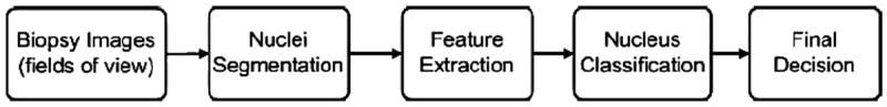
A typical flowchart of histopathology image-based computer-aided diagnosis.
One prominent characteristic of many of the methods that use nuclear morphometry to grade different kinds of cancers is that classification is performed using the naïve Bayes method whereby each nuclear structure (represented by a set of numerical features) is often classified independently from one another [16,17,11]. The set of nuclei extracted from a patient is then usually classified by using the majority voting (MV), or taking the most common class assignment, or perhaps by using different moments (e.g. mean, variance) of the distribution of nuclei. Thus any statistical dependency, such as correlation for example, between nearby structures is discarded. Several attempts to capture the spatial information between nearby cells from microscopic images have been made by using the graph theory [18,13]. In these works the x, y position of each nuclear structure in a field of view is used to generate a neighborhood graph which, together with average nuclear features, is used in an attempt to differentiate different classes. Information regarding the intricate distribution of the numerical features describing each structure, as well as co-dependencies between these in nearby nuclei, however, are often not used explicitly.
Our goal in this methodological note is to demonstrate that any amount of statistical dependency between the morphological characteristics of nearby nuclei can be utilized to improve the classification accuracy of methods usually employed for cancer diagnosis and differentiation. It is well known that cells in living tissues utilize several mechanisms (e.g. autocrine or paracrine) to ‘communicate’ with one another. Given that well established cell communication mechanisms exist, it could then be possible that the morphological information of a given nucleus could depend (statistically speaking) on the morphology of nearby nuclei. Here we present evidence that indeed numerical features of nuclei are more correlated to features extracted from nearby nuclei rather than those of distant nuclei, and that this difference is statistically significant. We then describe a method that utilizes any dependency present to augment the accuracy of classification (e.g. benign vs. malignant) in comparison with the naïve Bayes strategy (e.g. majority voting).
We note that the idea of classifying sets of samples (nuclei), rather than individual samples, is not new and has been studied in pattern recognition domains recently. In multiple instance learning (MIL) algorithms, for example, [19,20], the learner receives a set of bags (each containing more than one sample) that are labeled positive or negative. Here each bag is labeled, and not each sample. In MIL algorithms, however, a bag is labeled negative if all the instances in it are negative, but a bag is labeled positive if there is at least one instance in it which is positive. Other than MIL algorithms, [21], for example, investigated different instance learning methods, focusing on the classifier model construction. Under the same context, [17] proposed a K-nearest neighbor method for group-based classification by combining a MV scheme and a pooling scheme. They indicate that knowing a set of test samples that belong to the same, but unknown, class can be used to effectively reduce the individual Bayes error rate. Similar approaches that combine individual classification methods with the MV strategy were also investigated in the high-throughput applications [22,23] and revealed an improved classification performance compared to those not using MV strategy. In a similar manner, the method we describe below makes use of the spatial x, y position of nuclei in a field of view to exploit their dependency for augmented classification accuracies. We demonstrate the performance of our approach by classifying three types of thyroid lesions from 78 patients.
The remainder of this paper is structured as follows. In Section 2, we describe the mathematical model for the set classification problem, and show the relationship between the MV strategy and the likelihood ratio test (LRT) strategy. We then describe a method that is able to utilize ‘sets of nuclei’ extracted from image neighborhoods instead of individual nuclei. We note the new method does not require a specific ordering within each sub-group. Section 3 describes the computational procedures we utilized to demonstrate the application of our approach. Section 4 presents experimental results comparing the several computational strategies involved. Finally, summary and conclusions are offered in the last section of this document.
2. Bayesian framework
Let be a d-dimensional numerical feature vector describing the jth nucleus of the ith patient, and let describe the set of feature vectors pertaining to all nuclei belonging to the ith patient. Given a set of nuclear measurements Xi, the objective in pathology problems is to determine the class label y ∈ {y1, y2, …, yk} (for a problem with k gradings or classes) for this set of measurements. The maximum a posterior (MAP) criterion can be used to estimate the label of the set Xi via:
| (1) |
For a two-class problem, the label could be simply determined by comparing the posterior probabilities, given by
| (2) |
and testing whether this ratio is smaller or greater than one. By assuming the prior probability of each class is equal, i.e. p(y1) = p(y2) (when no a priori information regarding incidence is available), the likelihood ration test (LRT) [24] can be further simplified as
| (3) |
| (4) |
Computing the joint conditional probability is often difficult given the low number of samples in comparison with the number of dimensions (d × ni) that this would involve. The naïve Bayes assumption is then often used to overcome this problem. In this approach, it is assumed that the samples (nuclei) are independent from one another, i.e. . Under this assumption, the log-likelihood ratio in Eq. (3) can be computed as
| (5) |
Another approach that is often used in these situations is the MV strategy [25]. The main idea is to classify each sample in the case individually by using a chosen classifier, label each sample accordingly, and then assign the label with the majority of votes as the final label for the case (patient). In order to analyze the connection between MV and LRT, let the output of an individual classifier be , and define an indicator function as
| (6) |
where 1 denotes class y1, and 0 refers to class y2. Then the class label for the case Xi is determined by calculating the numbers of samples belonging to each class
| (7) |
Note that if is defined as the log-ratio of the posterior probabilities, then we could obtain similar functions as in Eqs. (3) and (4),
| (8) |
| (9) |
We can thus make a connection between the MV and the LRT under the naïve Bayes assumption. The MV strategy uses an indicator function to truncate the ‘soft’ assignments in the LRT.
2.1. Illustrating shortcomings of the naïve Bayes method
Although naïve Bayes approaches seem to work well in many applications, it is easy to see why it may not be optimal at times, especially when strong dependencies between samples (nuclei) may be present. Here we describe an illustrative example for this situation. Suppose our problem consists of determining whether nuclei from a given patient can be classified as benign (class 1) or malignant (class 2), and suppose we were using only one feature (e.g. nuclear area) to characterize each nucleus. Now, for the sake of argument, allow nuclei which are nearby each other in class 1 to have strong correlation with each other. That is, every time a nucleus with a large area is encountered, the chance that the nucleus closest to it also has a large area is high. Now suppose the situation is reversed for class 2. That is, every time a nucleus with large area is encountered, the chances are high that its neighboring nucleus would have a small area. This situation is depicted in Fig. 2(a). Now suppose we were attempting to classify this dataset utilizing the naïve Bayes method. With this method, we would assume independence between samples and utilize a one dimensional distribution for each class, see Fig. 2(b). In this situation one can see the classes are indistinguishable from one another irrespective of whether we would try to classify the data using the LRT or MV methods described in the previous section, or whether we would try to classify the data using moments (e.g. mean, variance) of these one dimensional distributions. On the other hand, if we consider pairs of nearby nuclei instead the data could be classified at a rate better than random assignment (e.g. using a K-nearest neighbor method), given that only a portion of the nuclear pairs overlap (near the center of plot Fig. 2(a)).
Fig. 2.
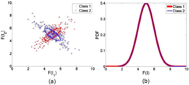
Illustration of group of nuclei distribution and individual nucleus distribution. (a) Each point represents one single group with two nuclei, and the two axes refer to the single feature for the two nuclei, respectively. Nuclei in each group are highly correlated and the distribution of groups are identical and independent from each class; (b) Distribution of individual nuclei based on the same feature.
2.2. New method for classification using spatial dependency
Here we describe a method to classify sets of nuclei extracted from each patient that can take advantage of any local dependencies. The method assumes there may be dependency between nuclei that are nearby each other in the tissue, while it assumes that nuclei far away from each other have no shared dependency. Let Z = {Z1, Z2, …, ZM} represent the set of nuclei pertaining to one patient, but now let each Zk correspond to sets of nuclei extracted from local image fields of view. That is, each set Zk contains n nuclei (with n − 1 a parameter to be chosen, a nucleus together with its n − 1 closest neighbors form a set). See Fig. 4 for an example where the group size is set to n = 5. Given the assumption of local dependency we have then that p(Z∣yj) = p(Z1∣yj)p(Z2∣yj) ⋯ p(ZM∣yj). We can compute p(Zk∣yk) using training data which in our case consist of similar neighborhoods chosen from the available patient database. An approximate value for p(Zk∣yk) can be computed using a kernel density-based approximation, or a K-nearest neighbor method. Below we provide computational examples using both approaches. To that end, all that is necessary is a way to estimate the distance measure D(Zk, Zm) between sets of nuclei (rather than individual nuclei). Having such a distance would allow us to compute p(Zk∣yk) as
| (10) |
where refer to the set of neighborhoods extracted from patients of class yj, and σ2 refers to the width of the kernel, and Nyj represents the number of groups (sets) of nuclei for class yj available in the training dataset.
Fig. 4.
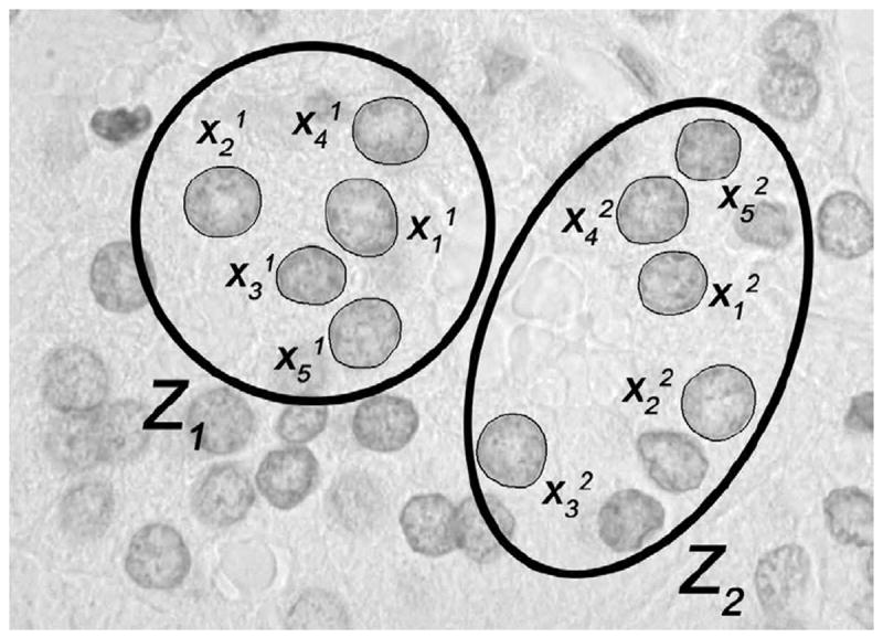
Illustration of cell grouping procedure where the number of nuclei per group is five.
We note that it is not possible to define a precise order in the nuclei that compose each neighborhood set Zk. This is due to arbitrary (or unknown) rotation that the set of nuclei may find themselves once imaged within a field of view. We therefore seek to minimize these effects by utilizing the earth mover’s distance (EMD) [26,27] to measure how close or far two sets of samples Zk and Zm are from one another. We note that in our case, the size (number of nuclei) in each group is kept constant, and therefore the EMD minimization can be written as
| (11) |
subject to the following constraints fuν ≥ 0, , , as well as:
| (12) |
Here the symbol du,ν denotes the feature space distance (described in more detail below) between two individual nuclei u (from group Zk) and ν (from group Zm), while fu,ν denotes how much ‘mass’ must be ‘transported’ between the two samples. See Fig. 3 for a schematic illustration. Eq. (11) represents a linear program which we minimize using the approach described in [27].
Fig. 3.
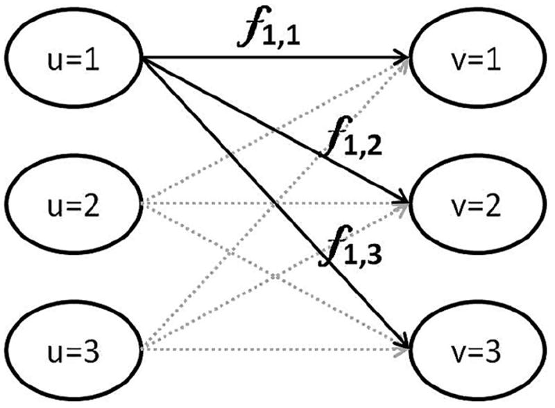
Schematic illustration of earth mover’s distance computation. Samples (nuclei) from the left side (with indices u = 1, 2, 3) are transported to the configuration on the right side so as to minimize the total amount of work (mass times distance).
Note that the transportation plan matrix fu,ν, u, ν = 1, …, n is a square matrix representing how much is being ‘transported’ (or moved) from index u to ν. The set of admissible matrices have the property that their entries must be between zero and one, and their sum along each column or row is one (bistochastic). They form a convex set [28] and the following theorem can be useful in interpreting this phenomenon:
Theorem 2.1
The set of extreme points of the set of bistochastic matrices coincides with the set of permutation matrices. In particular, the set of bistochastic measures is a polyhedron with n! vertices and every bistochastic matrix is a convex combination of permutation matrices.
A proof can be found in [28]. As a consequence, for any group size n, the solution for the optimal transport problem stated in (11) is a permutation matrix defining the correspondence between each nucleus in the sets Zk and Zm. This ‘registration’ in feature space allows for meaningful comparisons between sets of nuclei without needing to know which nucleus corresponds to which, thus avoiding issues with arbitrary rotation (for example).
To summarize, we seek to classify sets of nuclei pertaining to a single patient without using the naïve Bayes methodology and instead seek to exploit statistical dependency between nearby samples. To that end we first extract sub-groups of nuclei chosen from neighborhoods within a field of view. We then assume that there may be statistical dependencies between nuclei within each group. In addition, we assume that statistical dependencies between nuclei from different groups (far away from each other) are approximately zero. To estimate the probability of observing a specific set of nuclei we utilize the EMD distance (11). With a distance between sets in hand, we are now able to apply the standard kernel density estimation (KDE) as well as the popular K- nearest neighbor (K-NN) between sets of nuclei, rather than individual nuclei for estimating p(Zk∣yk). The class of an unknown set of nuclei is then estimated using Eq. (3). Below we demonstrate the application of the method using both the KDE and K-NN approaches, and compare them to the standard naïve Bayes approach.
3. Experimental setup
3.1. Dataset
In order to test the effectiveness of our approach, we tested the proposed methodology for classification of different thyroid lesions. The follicular lesions of the thyroid are selected in this study, since they remain significant diagnostic challenges in surgical pathology. Our dataset consists of three different types of thyroid lesions, namely follicular adenoma of the thyroid (FA), follicular variant of papillary thyroid carcinoma (FVPC), and nodular goiter (NG). While FVPC has familiar nuclear morphological features that are helpful diagnostically; these features (e.g. nuclear contour abnormalities) are not specific and are not always present. In addition, concerning other follicular lesions of the thyroid, nuclear features are not particularly helpful and not utilized for diagnostic determination. In the end, distinguishing between these entities is difficult even for experts in thyroid pathology.
Cases were reviewed by more than one pathologist who either specializes in thyroid pathology or head and neck pathology (at time of diagnosis). Lesions were reviewed for the study (J.A.O) and appropriate representative blocks, which contain lesions FA, FVPC or NG, selected for staining and image acquisition. Tissue blocks for each type were obtained from the archives of the University of Pittsburgh Medical Center (Institutional Review Board approval #PRO09020278). In this dataset, there are 28 patients for each FA and NG type of lesions, which have 609 and 584 fields of view, respectively and 22 patients for FVPC containing 572 fields of view. All images used for analysis in this study were acquired using an Olympus BX51 microscope equipped with a 100X UIS2 objective (Olympus America, Central Valley, PA) and 2 mega pixel SPOT Insight camera (Diagnostic Instruments, Sterling Heights, MI). Image specifications were 24bit RGB channels and 0.074 microns/pixel, 118 × 89 μm field of view.
3.2. Nuclear segmentation
The segmentation method described in [29,30] was employed to segment nuclei from each field of view. This method is based on supervised statistical modeling, which utilizes example input structures to learn a statistical model of the shape and texture of the structures to be segmented. From a new field of view, each nucleus is then segmented by maximizing the normalized cross correlation between the model and neighborhoods in the slide image and is adjusted through non-rigid registration. With the segmented nuclei images from the field of views, we computed the geometric center of the nuclei and obtained the relative coordinates of the centroids in the field of view as the center of each nucleus. After segmentation, the nuclear dataset consisted of 10958,10182, and 6997 segmented nuclei for classes FA, NG, and FVPC, respectively.
3.3. Feature extraction
Morphological and texture features were extracted for each segmented nucleus. In total, 256 numerical features were extracted per nucleus as follows:
MorphologicalFeatures: Nuclear morphological features are widely used in discriminating cancer cells from normal ones in image analysis in digital pathology [31]. We extracted six of the most popular features in our experiment: area, convexity, circularity, perimeter, eccentricity and equivalent diameter.
TextureFeatures: We computed three intensity-derived features (average intensity, standard deviation, and entropy), Haralick features and Gabor features as described in [32,33,11]. Using these techniques we computed 220 texture features in total for each nuclear image.
WaveletFeatures: Wavelet decomposition features can capture multi resolution information from images. We computed wavelet features as described in [11], which resulted in 30 features for each nuclear image.
Following the feature extraction procedure, the individual features were normalized by subtracting their mean and dividing by the standard deviation. As a result, each normalized feature set has mean 0 and standard deviation 1. The mean and standard deviation of each feature were computed from the training set of data during cross validation step, which is detailed in the following section.
3.4. Blind cross validation
In the results reported below we tested the ability of several methods to recover the correct label of each patient data sample. To that end, we applied a standard ‘leave one out’ cross validation (LOOCV) strategy. In our framework, we applied a ‘double cross validation’ methodology whereby a patient (case) is left out, and a classifier is trained using the remaining patients. In training the classifier, the training set is again split into a training and testing procedure to select the optimal relevant parameters (K in K-NN, σ in KDE, as well as the group size n). The selected optimal parameter combination is then used to determine the class of the patient in the test set according to Section 2.2. The stepwise discriminant analysis (SDA) [34] technique is first applied to the remaining training data and the parameters of the classifiers estimated using an exhaustive search procedure [24]. We notice that the number of groups in each class can be different in each ‘fold’. In order to avoid biases, we restrict the number of patients, as well as the number of groups, belonging to each class to be the same in the training set by randomly drawing from the entire set.
4. Results
4.1. Is there evidence for local spatial dependency between nuclear features?
We have sought to determine whether there is any evidence to believe that the nuclear features describing each extracted nucleus are dependent on nearby features, relative to any dependency between nuclei far away from each other. To that end, we utilized the entire set of extracted nuclear features and computed the feature corresponding to the first direction of the principal component analysis (PCA) technique applied to the entire feature space. Thus each nucleus was reduced to one numerical feature using the PCA technique. We then extracted pairs of nuclei (one nucleus and its nearest neighbor in that field of view) and computed Pearson’s correlation coefficient between their PCA-derived features. For comparison purposes, we also computed the correlation coefficient between pairs of nuclei chosen to be far apart from each other (different fields of view). The experiment (correlation coefficient computation) was repeated 20 times using random draws with replacement (each draw consisted of number of pairs equal to the number of nuclei per image) and the mean correlation coefficient is reported in Table 1 for both nearest and far away nuclei. Although the average correlation is low, the difference in means for the correlation coefficient computed using neighbor and non-neighbor cells is statistically significant (according to the standard Student’s t-test), indicating the nearby samples may be statistically dependent.
Table 1.
The average correlation coefficient between two sets of cells over all patients of cancer type FVPC, NG and FA.
| FVPC | NG | FA | |
|---|---|---|---|
| Between the nearest cells | 0.149 | 0.133 | 0.119 |
| Between the non-neighborhood cells | −0.010 | −0.050 | −0.020 |
| p-Value | 4.29 × 10⁻⁷ | 7.96 × 10⁻⁵ | 5.17 × 10⁻⁶ |
We clarify that our purpose here is simply to uncover evidence for statistical dependency between nearby nuclei. We do so by examining correlations between nearby nuclei (more precisely in their corresponding PCA-derived features) in comparison to correlations between nuclei which are far away from each other. Keeping in mind that it is possible for two random variables to be perfectly uncorrelated while still being statistically dependent, the actual correlation value is not the most important feature of the analysis, but rather the fact that this correlation value is statistically significantly higher for nearby cells in comparison to far away cells.
4.2. Comparison of classification results
Table 2 shows the average classification accuracy in differentiating FVPC and NG patients. The table shows average classification results utilizing both naïve Bayes and the new group-based approach discussed earlier. The averages were computed on 30 individual executions. For each individual execution, random nuclei are selected for training. Note that, we select random nuclei from each class to restrict the number of patients, as well as the number of groups, belonging to each class to be the same in the training procedure.
Table 2.
Classification accuracy comparison on FVPC vs. NG (%).
| FVPC | NG | Average | Cohen’s Kappa | |
|---|---|---|---|---|
| Naïve Bayes KDE | 71.82 ± 6.8 | 66.67 ± 5.7 | 68.93 ± 4.3 | 0.38 ± 0.09 |
| Group KDE | 81.97 ± 4.8 | 68.45 ± 3.0 | 74.40 ± 2.9 | 0.49 ± 0.06 |
| Naïve Bayes KNN | 84.70 ± 4.0 | 57.98 ± 4.4 | 69.73 ± 3.6 | 0.41 ± 0.07 |
| Group KNN | 89.39 ± 4.2 | 64.64 ± 2.5 | 75.53 ± 1.9 | 0.52 ± 0.04 |
For comparison purposes the comparisons using both KDE as well as the KNN methods are shown. In these tables, Naïve Bayes KDE stands for the standard method (assuming independence) while ‘Group KDE’ show results using our method described in Section 2.2. Similarly, Naïve Bayes KNN refers to the usual method and ‘Group KNN’ represents the method we described earlier. For brevity, only the diagonal of the confusion matrices are shown. That is, in this table, 71.82 percent of the actual FVPC patients were classified as so using the KDE approach. The average classification accuracy (average of diagonal of classification table) is reported in column 3. Finally, Cohen’s Kappa statistic [35] (another measure often using in quantifying the agreement with the gold standard) is reported on column 4. Table 3 contains the same data for the FA vs. NG diagnostic challenge. One can see that for both diagnostic challenges, and whether one is using the KNN or KDE techniques for estimating the related probabilities, on average, the naïve Bayes underperforms the method that takes into account local dependencies.
Table 3.
Classification accuracy comparison on FA vs. NG (%).
| FA | NG | Average | Cohen’s Kappa | |
|---|---|---|---|---|
| Naïve Bayes KDE | 75.48 ± 4.9 | 63.33 ± 5.1 | 69.41 ± 3.2 | 0.39 ± 0.07 |
| Group KDE | 78.93 ± 4.2 | 69.76 ± 3.5 | 74.35 ± 2.5 | 0.49 ± 0.05 |
| Naïve Bayes KNN | 73.21 ± 4.0 | 75.60 ± 2.8 | 74.40 ± 2.8 | 0.49 ± 0.05 |
| Group KNN | 82.26 ± 2.4 | 71.07 ± 2.7 | 76.67 ± 2.0 | 0.53 ± 0.04 |
Having 30 individual results of both approaches for both challenges, we were able to analyze the significance between proposed method and naïve Bayes methods. According to the standard Student’s t-test the improvement gained by our approach is statistically significant with α = 0.01 (p < 0.01). Based on the average and standard deviation of 30 individual executions, one can also say that proposed approach is robust with a low variation.
5. Summary and conclusions
Our goal in this methodological note was to demonstrate the potential for existence of statistical dependency of nuclear features in nearby nuclei, and describe a method that is able to utilize this for improved classification accuracy. We first derived a relationship between the popular MV and LRT strategies for classifying sets of nuclei in relation to the naïve Bayes approach. We then described a method for classifying sets of nuclei that first groups nuclei which are within a certain neighborhood within a given field of view. Groups (sets) of nuclei extracted from a given patient are classified utilizing the LRT that compares the extracted groups to groups already present in the training data. Our method utilizes EMD between sets of numerical features to make this comparison meaningful. We note that the EMD has already been used in image analysis problems in the past [26,27], and here we have adapted the technique to exploit local dependency in pathology datasets. Results utilizing real patient data of thyroid lesions show that, on average, a few percentage points in classification accuracy can be obtained. Comparisons were performed utilizing both KDE and K-NN techniques for estimating the related probabilities and similar improvements were found in both cases. We also note that these improvements, however, are likely to manifest themselves differently in different malignancies, as well as datasets.
In addition, though we have used the EMD concept for comparing sets of nuclei, in this context, the strategy is equivalent to comparing all possible parings of nuclei between two groups, and choosing the pairing for which the sum of distances between each pair is smallest (see Theorem 2.1). This provides a way to ‘register’ the sets of nuclei in feature space. However, since the overall complexity of computing the EMD between two sets of nuclei is roughly n3, the associated cost of the computation can be high for large databases.
We also note an important limitation of the approach we presented here. Although the method we described was successful in augmenting classification accuracy in cancer detection in a statistically significant manner, by itself, it sheds no light into the form (e.g. shape, texture, etc.) that this dependency is reflected in nuclear phenotypes. The ‘toy’ example provided in Section 2.1 (Fig. 2) serves only to illustrate the idea, and by no means reflect actual dependencies which may be encountered. We also postulate that the form that these dependencies take place could also vary case by case, as well as in different tissues and cancer types. Future work will focus on utilizing modern transport-based image analysis approaches [36] to decode the spatial and statistical dependency of the shape and texture information in nuclear structures in several cancers.
Finally, we note that although we have applied the technique to nuclear structure-based pathology based on histological imaging, the technique could be applied to any (sub) cellular phenotype that can be segmented and measured. This includes vesicular protein patterns imaged utilizing bright light microscopy as well as fluorescence microscopy, for example.
Acknowledgments
We wish to thank Drs. Badrinath Roysam, Yousef Al-Kofahi, and Dejan Slepcev for discussions on related topics. Akif B. Tosun and Gustavo K. Rohde’s work was partially supported by Pennsylvania State Health Department award 4100059192.
Footnotes
This work was supported in part by NIH awards R21GM088816, R01GM090033.
This paper has been recommended for acceptance by C. Luengo.
Contributor Information
Hu Huang, Email: huh@andrew.cmu.edu.
Akif Burak Tosun, Email: tosun@cmu.edu.
John A. Ozolek, Email: ozolja@upmc.edu.
Gustavo K. Rohde, Email: gustavor@cmu.edu.
References
- 1.Pienta K, Coffey D. Nuclear-cytoskeletal interactions: Evidence for physical connections between the nucleus and cell periphery and their alteration by transformation. J Cell Biochem. 1992;49:357–365. doi: 10.1002/jcb.240490406. [DOI] [PubMed] [Google Scholar]
- 2.Zink D, Fischer A, Nickerson J. Nuclear structure in cancer cells. Nat Rev Cancer. 2004;4:677–687. doi: 10.1038/nrc1430. [DOI] [PubMed] [Google Scholar]
- 3.Dey P. Cancer nucleus: morphology and beyond. Diagn Cytopathol. 2010;38:382–390. doi: 10.1002/dc.21234. [DOI] [PubMed] [Google Scholar]
- 4.Stenkvist B, Westman-Naeser S, Holmquist J, Nordin B, Bengtsson E, Vegelius J, Eriksson O, Fox C. Computerized nuclear morphometry as an objective method for characterizing human cancer cell populations. Cancer Res. 1978;38:4688–4697. [PubMed] [Google Scholar]
- 5.Bagui S, Bagui S, Pal K, Pal N. Breast cancer detection using rank nearest neighbor classification rules. Pattern Recognit. 2003;36:25–34. [Google Scholar]
- 6.Padfield D, Chen B, Roysam H, Cline C, Lin G, Seel M. Cancer tissue classification using nuclear feature measurements from dapi stained images. Proceedings of First Workshop on Microscopic Image Analysis with Applications in Biology; pp. 86–92. [Google Scholar]
- 7.Basavanhally A, Ganesan S, Agner S, Monaco J, Feldman M, Tomaszewski J, Bhanot G, Madabhushi A. Computerized image-based detection and grading of lymphocytic infiltration in her2+ breast cancer histopathology. IEEE Trans Biomed Eng. 2010;57:642–653. doi: 10.1109/TBME.2009.2035305. [DOI] [PubMed] [Google Scholar]
- 8.Singh S, Gupta P. Breast cancer detection and classification using neural network. Int J Adv Eng Sci Technol. 2011;6:4–9. [Google Scholar]
- 9.Nagashima T, Suzuki M, Oshida M, Hashimoto H, Yagata H, Shishikura T, Koda K, Nakajima N. Morphometry in the cytologic evaluation of thyroid follicular lesions. Cancer Cytopathol. 1998;84:115–118. [PubMed] [Google Scholar]
- 10.Gupta N, Sarkar C, Singh R, Karak A. Evaluation of diagnostic efficiency of computerized image analysis based quantitative nuclear parameters in papillary and follicular thyroid tumors using paraffin-embedded tissue sections. Pathol Oncol Res. 2001;7:46–55. doi: 10.1007/BF03032605. [DOI] [PubMed] [Google Scholar]
- 11.Wang W, Ozolek J, Rohde G. Detection and classification of thyroid follicular lesions based on nuclear structure from histopathology images. Cytometry Part A. 2010;77:485–494. doi: 10.1002/cyto.a.20853. [DOI] [PMC free article] [PubMed] [Google Scholar]
- 12.Veltri R, Isharwal S, Miller M, Epstein J, Partin A. Nuclear roundness variance predicts prostate cancer progression, metastasis, and death: a prospective evaluation with up to 25 years of follow-up after radical prostatectomy. The Prostate. 2010;70:1333–1339. doi: 10.1002/pros.21168. [DOI] [PubMed] [Google Scholar]
- 13.Doyle S, Feldman M, Shih N, Tomaszewski J, Madabhushi A. Cascaded discrimination of normal, abnormal, and confounder classes in histopathology: Gleason grading of prostate cancer. BMC Bioinf. 2012;13:282. doi: 10.1186/1471-2105-13-282. [DOI] [PMC free article] [PubMed] [Google Scholar]
- 14.Ikeguchi M, Sato N, Hirooka Y, Kaibara N. Computerized nuclear morphometry of hepatocellular carcinoma and its relation to proliferative activity. J Surg Oncol. 1998;68:225–230. doi: 10.1002/(sici)1096-9098(199808)68:4<225::aid-jso4>3.0.co;2-6. [DOI] [PubMed] [Google Scholar]
- 15.Tosun AB, Gunduz-Demir C. Graph run-length matrices for histopathological image segmentation. IEEE Trans Med Imaging. 2011;30:721–732. doi: 10.1109/TMI.2010.2094200. [DOI] [PubMed] [Google Scholar]
- 16.Al-Kofahi Y, Lassoued W, Lee W, Roysam B. Improved automatic detection and segmentation of cell nuclei in histopathology images. IEEE Trans Biomed Eng. 2010;57:841–852. doi: 10.1109/TBME.2009.2035102. [DOI] [PubMed] [Google Scholar]
- 17.Samsudin N, Bradley A. Nearest neighbour group-based classification. Pattern Recognit. 2010;43:3458–3467. [Google Scholar]
- 18.Doyle S, Agner S, Madabhushi A, Feldman M, Tomaszewski J. Automated grading of breast cancer histopathology using spectral clustering with textural and architectural image features. Fifth IEEE International Symposium on Biomedical Imaging: From Nano to Macro, 2008, ISBI 2008, IEEE; 2008. pp. 496–499. [Google Scholar]
- 19.Andrews S, Tsochantaridis I, Hofmann T. Advances in Neural Information Processing Systems. Vol. 15. MIT Press; 2003. Support vector machines for multiple-instance learning; pp. 561–568. [Google Scholar]
- 20.Maron O, Lozano-Prez T. Advances In Neural Information Processing Systems. MIT Press; 1998. A framework for multiple-instance learning; pp. 570–576. [Google Scholar]
- 21.Ning X, Karypis G. The set classification problem and solution methods. IEEE International Conference on Data Mining Workshops, 2008, ICDMW’08, IEEE; 2008. pp. 720–729. [Google Scholar]
- 22.Sansone C, Paduano V, Ceccarelli M. Combining 2d and 3d features to classify protein mutants in hela cells. Mult Clas Syst. 2010:284–293. [Google Scholar]
- 23.Soda P, Onofri L, Iannello G. A decision support system for crithidia luciliae image classification. Artif Intell Med. 2011;51:67–74. doi: 10.1016/j.artmed.2010.05.005. [DOI] [PubMed] [Google Scholar]
- 24.Bishop C. Information Science and Statistics. Springer; 2006. Pattern Recognition and Machine Learning. [Google Scholar]
- 25.Lam L, Suen S. Application of majority voting to pattern recognition: An analysis of its behavior and performance. IEEE Trans Syst Man Cybern Part A Syst Hum. 1997;27:553–568. [Google Scholar]
- 26.Rubner Y, Tomasi C, Guibas L. The earth mover’s distance as a metric for image retrieval. Int J Comput Vis. 2000;40:99–121. [Google Scholar]
- 27.Wang W, Ozolek J, Slepcev D, Lee A, Chen C, Rohde G. An optimal transportation approach for nuclear structure-based pathology. IEEE Trans Med Imaging. 2011;30:621–631. doi: 10.1109/TMI.2010.2089693. [DOI] [PMC free article] [PubMed] [Google Scholar]
- 28.Carlier G. Lecture Notes. Institute for Mathematics and its Applications, University of Minnesota; 2010. Optimal transportation and economic applications. [Google Scholar]
- 29.Chen C, Wang W, Ozolek J, Lages N, Altschuler S, Wu L, Rohde G. A template matching approach for segmenting microscopy images. 2012 Ninth IEEE International Symposium on Biomedical Imaging (ISBI); 2012. pp. 768–771. [Google Scholar]
- 30.Chen A, Wang W, Ozolek JA, Rohde G. A flexible and robust approach for segmenting cell nuclei from 2d microscopy images using supervised learning and template matching. Cytom Part A. 2013;83:495–507. doi: 10.1002/cyto.a.22280. [DOI] [PMC free article] [PubMed] [Google Scholar]
- 31.Mahfouz S, El-Sharkawy S, Sharaf W, Hussein H, El-Nemr R. Image cytometry of fine needle aspiration of thyroid epithelial lesions. Appl Immunohistochem Mol Morphol. 2012;20:25. doi: 10.1097/PAI.0b013e31821ffa6a. [DOI] [PubMed] [Google Scholar]
- 32.Haralick R, Shanmugam K, Dinstein I. Textural features for image classification. IEEE Trans Syst Man Cybern. 1973:610–621. [Google Scholar]
- 33.Boland M, Murphy R. A neural network classifier capable of recognizing the patterns of all major subcellular structures in fluorescence microscope images of hela cells. Bioinformatics. 2001;17:1213–1223. doi: 10.1093/bioinformatics/17.12.1213. [DOI] [PubMed] [Google Scholar]
- 34.Jennrich RI, Sampson P. Stepwise discriminant analysis. Stat Methods Digital Comput. 1977;3:77–95. [Google Scholar]
- 35.Wood JM. Understanding and computing cohen’s kappa: a tutorial. WebPsychEmpiricist. 2007 Web Journal at: http://wpe.info/
- 36.Wang W, Slepčev D, Basu S, Ozolek JA, Rohde GK. A linear optimal transportation framework for quantifying and visualizing variations in sets of images. Int J Comput Vis. 2013;101:254–269. doi: 10.1007/s11263-012-0566-z. [DOI] [PMC free article] [PubMed] [Google Scholar]