Learning to Associate Auditory and Visual Stimuli: Behavioral and Neural Mechanisms

Abstract

The ability to effectively combine sensory inputs across modalities is vital for acquiring a unified percept of events. For example, watching a hammer hit a nail while simultaneously identifying the sound as originating from the event requires the ability to identify spatio-temporal congruencies and statistical regularities. In this study, we applied a reaction time (RT) and hazard function measure known as capacity (e.g., Townsend and Ashby, 1978) to quantify the extent to which observers learn paired associations between simple auditory and visual patterns in a model theoretic manner. As expected, results showed that learning was associated with an increase in accuracy, but more significantly, an increase in capacity. The aim of this study was to associate capacity measures of multisensory learning, with neural based measures, namely mean Global Field Power (GFP). We observed a co-variation between an increase in capacity, and a decrease in GFP amplitude as learning occurred. This suggests that capacity constitutes a reliable behavioral index of efficient energy expenditure in the neural domain.

The majority of our perceptions are derived from multiple sensory modalities. For example, when we see a talker’s face, we can obtain supplementary information from lip-reading to facilitate word and sentence comprehension. Each of these sensory inputs is combined into a unified percept. Such integration across modalities can result in significant behavioral benefits, including but not limited to faster response times (RTs) (e.g. Diederich & Colonius, 2004; Hershenson, 1962), enhanced detection rates (e.g. Lovelace, Stein, & Wallace, 2003), and improved spatial localization (e.g. Nelson et al., 1998). These processes are far from simple, however. One of the more substantial issues that must be overcome is known as the binding problem, originally defined by William James (James, 1890). At any given moment, there is a large quantity of incoming sensory information in each modality and a well-adapted perceptual system must be able to correctly bind sensory information that originates from a single source into a unified percept, but at the same time, must correctly segregate sensory information that originates from different sources.

The impact of stimulus factors in multisensory integration has been relatively well studied. Research originally using single unit recordings has identified three primary factors that modulate whether or not two sensory inputs are integrated, and whether there is a neural benefit relative to unisensory responses (also known as multisensory gain), concepts that have been generalized to studies of human neuroimaging, behavior, and perception.¹ The first factor is the spatial congruence of the auditory and visual inputs. The more spatially congruent the stimuli, the more likely they are to be perceptually bound and contribute to multisensory gain, a finding seen from animal neurophysiology (Meredith & Stein, 1986a, 1996; Wallace et al., 2004), human neuroimaging (Fiebelkorn, Foxe, Schwartz, & Molholm, 2010; Macaluso, George, Dolan, Spence, & Driver, 2004; Meredith & Stein, 1996), and human behavior and perception (Frens, Van Opstal, & Van der Willigen, 1995; Munhall & Vatikiotis-Bateson, 2004; Wallace et al., 2004). Similarly, the temporal coincidence of auditory and visual inputs influence integration; the more synchronous they are, the greater the probability of integration. Like the spatial principle, the temporal principle has been demonstrated in studies of animal neurophysiology (Meredith, Nemitz, & Stein, 1987; Wallace et al., 2004), human neuroimaging (James & Stevenson, 2012; Macaluso et al., 2004; Miller & D’Esposito, 2005; Stevenson, Altieri, Kim, Pisoni, & James, 2010; Stevenson, VanDerKlok, Pisoni, & James, 2011; Talsma, Senkowski, & Woldorff, 2009; van Atteveldt, Formisano, Blomert, & Goebel, 2007), and human behavior and perception (Colonius & Diederich, 2010; Conrey & Pisoni, 2006; Diederich & Colonius, 2009; Dixon & Spitz, 1980; Hillock, Powers, & Wallace, 2011; Keetels & Vroomen, 2005; van Wassenhove, Grant, & Poeppel, 2007; Zampini, Guest, Shore, & Spence, 2005).

Both the spatial and temporal factors are reflective of the statistics of the natural environment. The third stimulus factor is effectiveness, or the ability of a stimulus to drive a given response. Stimulus effectiveness modulates multisensory interactions in such a way that less salient stimuli produce greater multisensory enhancement relative to unisensory responses. This phenomenon is known as inverse effectiveness, which has again been demonstrated in animal neurophysiology (Meredith & Stein, 1986b; Stein, Stanford, Ramachandran, Perrault, & Rowland, 2009; Wallace, Wilkinson, & Stein, 1996), human neuroimaging (James, Stevenson, & Kim, 2012; Stevenson et al., 2012; Stevenson & James, 2009; Stevenson, Kim, & James, 2009), and human behavior (Altieri & Townsend, 2011; Hecht, Reiner, & Karni, 2008).

The benefits of multisensory integration can be seen not only with behavioral facilitation, but also with changes in the neural response properties. Congruency effects have been measured in a wide network of brain regions depending upon the tasks and stimuli used (Doehrmann & Naumer, 2008). For example, a collection of fMRI studies have identified inferior frontal cortex and superior temporal cortex as two primary regions showing such congruency effects with objects (Belardinelli et al., 2004; Hein et al., 2007; Noppeney, Josephs, Hocking, Price, & Friston, 2008) and speech (Calvert, Campbell, & Brammer, 2000; Ojanen et al., 2005; Pekkola et al., 2006; Stevenson et al., 2010; Stevenson et al., 2011; N. van Atteveldt, Formisano, Goebel, & Blomert, 2004; van Atteveldt, Formisano, Blomert, et al., 2007; van Atteveldt, Formisano, Goebel, & Blomert, 2007), though it should be noted that effects are not necessarily confined to these regions (Laurienti et al., 2003; Taylor, Moss, Stamatakis, & Tyler, 2006).

Multisensory Perceptual Training

The manner with which stimulus inputs are integrated across the senses can be rapidly changed with perceptual training. For example, the impact that temporal coincidence has on the binding of auditory and visual changes can be manipulated in laboratory settings. Through consistent presentations of slightly asynchronous stimuli, the window of temporal offsets in which an individual will perceptually bind audiovisual stimuli can be shifted (Vroomen, Keetles, de Gelder, and Bertelson, 2004). Similarly, perceptual feedback training can narrow the temporal binding window, increasing the temporal precision of individuals in making judgments about audiovisual relationships (Powers, Hevey, & Wallace, 2012; Powers, Hillock, & Wallace, 2009; Stevenson, Wilson, Powers, & Wallace, 2013). These examples of multisensory malleability show that even into adulthood, the mechanisms used to merge information across sensory modalities remains plastic. A study by Tanabe and colleagues (2005) used feedback training to teach participants to associate arbitrary pairs of temporally modulated noise and visual texture patterns. Using a delayed match-to-sample task, the authors showed a decrease in superior temporal sulcus activation subsequent to training (a known region of audiovisual integration; Beauchamp, Lee, Argall, & Martin, 2004; Calvert et al., 2000; James, VanDerKlok, Stevenson, & James, 2011; Stevenson, Geoghegan, & James, 2007; Stevenson et al., 2009). Importantly, this decrease was correlated with behavioral accuracy in identifying associated pairs, suggesting an increased efficiency of processing with learned audiovisual associations.

In the current study, we propose that an increase in capacity—a reaction time measure of efficiency—will result from a learned association between previously unassociated auditory and visual stimuli (auditory pure-tones and Gabor patches). We define “efficiency” in the neural and behavioral domains as the ability to complete a task in a finite amount of time when provided with a certain amount of perceptual channels or processing resources. Consider a multisensory matching task in which the participant must make a “yes” response when two stimuli correspond to one another. Assume the availability of auditory and visual information, as well as a certain amount of neural resources. Efficiency increases when participants are able to make correct responses faster or more accurately, given the information available. We measure efficiency using a RT measure of capacity (e.g., Townsend & Ashby, 1978; see also Wenger & Gibson, 2004) which will be described later.

In the neural domain, increases in efficiency should be reflected by a decrease in brain signals; that is, as one learns the task, less energy should have to be applied to distinguish the patterns that match from the ones that mismatch. Participants will be trained to make a “yes” response if and only if the frequency exhibited by the auditory pure tone and the Gabor Patch correspond to the trained match, and a “no” response otherwise. The purpose of this study is to observe co-variations between capacity as a statistical measure of multisensory learning, and brain activation, which index a change in the amount of energy expended by the neurocognitive system as learning occurs.

Methods: Modeling

Capacity: A Measure of Efficiency

Learning often involves becoming attuned to auditory, visual, or multimodal regularities (e.g., Saffran, Johnson, Aslin, and Newport, 1999; Seitz, Kim, van Wassenhove, and Shams, 2007), and the subsequent transfer of this knowledge to memory. Traditional assessments of learning rely on measuring changes in accuracy, or in the case of perceptual learning, mean changes in threshold across stages of practice (e.g., Altieri and Wenger, Under Review; Dosher, and Lu, 1999; McKee and Westheimer, 1978). Learning and memory are strongly associated with the notion of efficiency or capacity. For example, Capacity in memory has undergone a re-conceptualization over the years to include stages of learning and transfer via practice (e.g., Cowan, Elliot, Saults, Morey, Mattox, Hismjatullina, and Conway, 2005; see also Atkinson and Shiffrin, 1968). Nonetheless, capacity is often viewed as a fixed construct that does not change across time (cf. Townsend and Altieri, 2012).

A considerable body of literature has recast the notion of capacity as a measure of efficiency, using RT distributions (e.g., Townsend and Nozawa, 1995; Wenger and Gibson, 2004) or a combination of RTs and accuracy (Townsend and Altieri, 2012). As Wenger and Gibson (2004) argued, assessing capacity in terms of mean RTs or mean accuracy has several shortcomings. First, means provide only an expected value and therefore do not map well onto the notion of efficiency or capacity as a measure of system level performance. Second, cognitive processes involved in learning, memory, and recognition, expend some amount of energy and must be completed in a finite amount of time. Capacity is a measure that assesses the instantaneous amount of energy at a certain processing time expended to yield recognition.

Hazard Functions and Efficiency

An important component of our investigation centers on the implementation of a measure capturing the idea that learning involves the increasingly efficient use of cognitive resources. We accomplish this by measuring capacity and examining the data at the level of the hazard function. One way in which capacity may be measured, and the method favored here, involves obtaining the distribution of RTs from a given experimental condition (for example, from audiovisual trials, as done here), and computing the estimated hazard functions from the different conditions. The hazard function provides the probability that a process will be completed in the next instant in time, given that it has not completed already by time t. The hazard function may be written as:

$$h(t)=\underset{\mathrm{\Delta }t\to 0}{\lim }\frac{P(t\le T\le t+\mathrm{\Delta }t\mid T\ge t)}{\mathrm{\Delta }t},\mathrm{or\; simply},h(t)\frac{f(t)}{1-F(t)}.$$

The term f(t) denotes the probability density function, while F(t) is the cumulative probability density function yielding the probability that recognition has occurred by a certain time. The term in the denominator, 1-F(t), is a survivor function expressing the probability that a process has not completed by a certain time.

The use of hazard functions has been favored in the literature since they provide an estimate of the “intensity” or the instantaneous amount of work completed (Townsend and Ashby, 1978; see also Wenger and Gibson, 2004). Utilizing hazard functions affords several statistical advantages compared to using mean RTs or accuracy. As one example, Townsend (1990) proved that an ordering of hazard functions from two experimental conditions (A and B) such that h_A(t) > h_B(t) implies not only greater work completed in condition A relative to B, but also an ordering of the means from those conditions. However, the converse is not always true—an ordering of means does not imply an ordering of hazard functions.

Cox Regression

One potential disadvantage to using hazard functions concerns the difficulty associated with hazard function estimation (Luce, 1986). While several remedies have been proposed (see Wenger and Gibson, 2004; Wenger et al., 2010), we shall employ a semi-parametric regression procedure known as Cox proportional hazard models (Cox, 1972). The purpose of proportional hazard model regression is to test for ordering of two or more hazard functions derived from different experimental conditions. Cox regression essentially transforms the proportional hazard functions into linear regression. Here, an independent variable (i.e., experimental conditions) may serve as a predictor, while the RTs obtained from these conditions serve as the data or “y” variable. Proportional hazard model regression is based on a log-linear regression procedure, and the method implemented here uses a specific class of models known in the literature as the fixed-effects partial likelihood approach (e.g., Allison, 1996). Specifically, it is assumed that the underlying hazard function for the j^th trial in participant 1 at time can be written as ln[h_1j(t)] = βx_1j(t) + α₁(t) + ε₁. The term α₁(t) denotes a baseline hazard function particular to that observer, and x_1j(t) represents one of the experimental factors, in our case the training day, that could influence the rate of processing on a given trial. The weight β represents the relative strength or influence of this factor. Finally, ε₁ denotes the unobservable heterogeneity particular that that individual, although this can be absorbed into the baseline hazard, giving us ln[h_1j(t)] = βx_1j(t) + α₁(t).

One benefit to the hazard function approach is that few parametric assumptions regarding the underlying distribution of the data need to be made. The only major requirement relates to the assumption of proportionality between the hazard functions from two or more experimental conditions (see Wenger and Gibson, 2004). In the context of our specific case, the underlying hazard functions across days of learning must be proportional to each other. For example, the hazard functions for days 1 and 2 for a given individual should be h₁(t) = γh₂(t), where γ reflects a constant of proportionality that remains invariant across trials, time, and experimental trials. As we shall demonstrate, the data within each of our participants reflects this assumption. One graphical test for the proportionality assumption begins with the fact that since h₁(t) = γh₂(t), it must also be true that H₁(t) = γH₂(t). Then, because we know that the integrated hazard function H(t) = -ln[S(t)] (where (S(t) = 1 − F(t), or 1 − CDF), we can arrive at the following formula: - ln[S₁(t)] = γ{-ln[S₂(t)]}. Finally, we obtain the log of both sides to get ln[-ln[S₁(t)]] = ln[γ] + ln{-ln[S₂(t)]}.

Conveniently, many common statistical packages (e.g., R and Matlab) allow one to apply the proportional hazard model test. Second, it requires few assumptions, the major one being that the underlying hazard functions are proportional to one another (which can be tested as we discuss later). Furthermore, unlike many statistical tests such as a z-test, the proportional hazard model does not make assumption regarding the parametric form of the underlying RT distribution. As an example, it does not require researchers to assume a normal distribution in the data. In this study, we assessed learning in the contextual framework of capacity by measuring capacity and implementing the Cox proportional hazard model. The hypothesis was that as participants learned the association across days (the regression variable) as a result of practice, RTs would decrease, and hence, the instantaneous amount of work completed measured by proportional hazards would increase.

Methods: Experimental Design

The purpose of this study involved analyzing the EEG signal (a time based neural measure) in conjunction with capacity as a function of learning across days. Because capacity constitutes a behaviorally based measure of energy expenditure, we expected to uncover distinct neural covariates of efficiency in terms of “work completed”. Specifically, as capacity increases as observers learn the association between the auditory and visual patterns, we expect to find a corresponding decrease in the amplitude of the EEG signal between the conditions in which the components matched versus when the components were mismatched. Hence, we predict that the energy required to discriminate the matched versus mismatched signals should decrease across days as observers show evidence for learning (see e.g., Stevenson et al., 2007, for an analogue using fMRI). Specifically, we predicted a co-variation between mean Global Field Power (GFP)—a measure of spatial standard deviation (e.g., Skrandies, 1990), and capacity. As capacity increases, the difference in GFP between the matched versus mismatched AV signal should decrease. Capacity should essentially index a perceptual component mirroring increasingly efficient use of neural resources as learning unfolds.

Finally, a significant motivation for the predicted co-variation between behavioral and neural measures of efficiency lies in recent findings suggesting that capacity is a superior predictor of the integrity of neural circuits pertinent to episodic memory compared to mean RT or accuracy (Wenger, Negash, Petersen, and Petersen, 2010). Wenger et al. (2010) carried out an analysis of capacity in an episodic cued memory task using aging participants. The authors found that the performance of a computational model of a hippocampal circuit, as a function of different levels of degradation, was a superior predictor of capacity scores (compared to mean RT and accuracy) in normal aging, MCI (mild cognitive impairment), and participants with dementia of the Alzheimer’s type.

Participants

Four right-handed college-aged observers were recruited from The University of Oklahoma campus and paid for their participation (mean age = 21). Each of the observers had normal or corrected-to-normal vision and reported no history of hearing or cognitive impairment. Participants were naïve regarding the purpose of the study. This study was approved by the University of Oklahoma Institutional Review Board and meets the qualifications for ethical research participation.

Materials

The visual stimuli consisted of diagonally oriented (45°) Gabor patches presented foveally in the center of the screen. Figure 1 shows examples of the six Gabor gratings presented in the audiovisual task. Stimuli were created on a continuum ranging from “low” to “high” frequency in six step sizes. The lowest frequency Gabor patch was created at 4 Hz, followed by 5 Hz, 6.6 Hz, 8.3 Hz, 12.5 Hz, up to the highest frequency of 25 Hz. The stimuli were designed in such a way as to create perceptually similar step sizes in frequency at each point in the continuum. Stimuli were presented centered on a 4 × 4 inch square with a luminance of 75 cd/m² at a background luminance level of 46 cd/m². Experimental stimuli were presented on a gamma-corrected computer CRT monitor.

Figure 1.

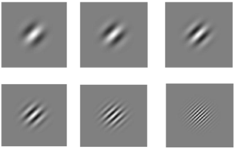
Gabor patches oriented diagonally. The visual stimuli, when present consisted of 1 of 6 levels of frequency as shown in this figure. From the top left to the bottom right cycles in Hz: 4 Hz, 5 Hz, 6.6 Hz, 8.3 Hz, 12.5 Hz, and 25 Hz. Auditory pure tones were created at 400 Hz, 500 Hz, 660 Hz, 830 Hz, 1250 Hz, and 2500 Hz.

The auditory stimuli consisted of digitized pure tones created in Matlab. The tones were presented at approximately 68 dB SPL over speakers positioned to each side of the participant in a quiet, sound attenuated booth. Similar to the visual stimuli, the tones were created on a six-step continuum ranging from “low” to “high” frequency. The lowest frequency tone was digitized at 400 Hz, followed by 500 Hz, 660 Hz, 830 Hz, 1250 Hz, and finally, 2500 Hz.

The auditory and visual stimulus components were factorially combined at each level (6-visual × 6-auditory) for a total of 36 unique audiovisual trial types. Auditory and visual-only trials were presented as well, for a total of 48 trial types. Stimuli were presented in a completely darkened sound attenuated chamber and were all 100 ms in duration and simultaneously presented. Participants were seated 76 cm from the monitor and their chins were placed comfortably on a chin rest.

Procedure

The experiment required 7 days for each observer. Each experimental session lasted approximately 45-60 minutes. Observers participated in one session per day with a total of 600 trials per day (120 A-only with 20 at each frequency, 120 V-only with 20 at each frequency, 120 AV when frequencies matched, and 240 AV trials when the frequencies mismatched).² Each experimental trial began with a black dot appearing in the center of a white background on the computer monitor. This was the cue for the participant to initiate the experimental trial by pressing the left button on the button pad in front of them. The initiation of each trial began with a random fore period of 100-500 ms followed by either an audiovisual, auditory-only, or visual-only trial.

Audiovisual trials consisted of a simultaneously presented tone and Gabor patch. Of the 360 AV trials presented per session, 120 of these were trials in which the frequency components matched (i.e., were associated). Because the purpose of this study involved teaching participants to associate auditory and visual images in terms of physical stimulus properties, participants were instructed to respond by pressing the right button labeled YES as quickly and as accurately as possible when the frequency of the auditory and visual modalities were associated (see below for a description of the method of association). The diagonal columns (in bold) in Table 1 show the total number of each type of “yes” trials for each cell in which the auditory and visual frequency components matched. The off-diagonal columns show the cases in which auditory and visual information were presented but did not match. Participants were instructed to respond “no” on these trails. On the auditory-only trials, the tone was presented with a static gray square. On the visual-only trials, a Gabor patch was presented without an accompanying sound. Participants were required to make a “no” response on unisensory trials. RTs and accuracy were collected from both “yes” and “no” trials and utilized in the subsequent data analysis. At the beginning of each day, participants were presented with 48 practice trials with at least 1 trial from each type in order to orient them with the response mappings. Our data analyses focused on the audiovisual trials.

Table 1.

This table shows the total number of trials presented for each stimulus configuration. That is, there are 36 AV stimuli, plus 6 A-only and 6 V-only for a total of 48 trial types. The columns on the diagonal (in bold) correspond to the “yes” trials in which the frequency of the Gabor patch and tone match.

	V1	V2	V3	V4	V5	V6	A-only
A1	140	56	56	56	56	56	140
A2	56	140	56	56	56	56	140
A3	56	56	140	56	56	56	140
A4	56	56	56	140	56	56	140
A5	56	56	56	56	140	56	140
A6	56	56	56	56	56	140	140
V-Only	140	140	140	140	140	140

Method of Association

Both auditory pure tones and Gabor patches were categorized on a 6-step “frequency” continuum, as shown in Table 1. A tone-Gabor patch pair was deemed to match if their frequency levels corresponded. The Gabor patch with the lowest frequency grating was arbitrarily matched with the lowest pitch tone while the Gabor patch with the highest frequency grating was matched with the highest pitch tone, and so on. Feedback was provided immediately after each trial (both matched and mismatched trials) informing the participant whether their response was correct or incorrect.

EEG Recordings

EEG recordings were made with an EGI NetStation system using a dense electrode 128-channel net (Electro Geodesics International, Eugene, OR). Data were continuously acquired throughout each testing session with a sampling rate of 1 kHZ. Electrodes were referenced to the central electrode (Cz). Two electrodes, one located under each eye monitored eye movements, and a set of electrodes placed near the jaw were used for off-line artifact rejection. Channel impedances were maintained at 50 K Ohms or under for the duration of the session.

EEG Analysis

After down sampling the data to 250 Hz to reduce the size of the data sets, a visual inspection was carried out to determine whether any channels were exceptionally noisy. Subsequent to inspection, all channels were maintained in the analyses. Artifacts resulting from facial movement were eliminated using an automated thresholding procedure from EEGLab. The mean proportion of trials retained across participants was greater than .90 (.92 for the matched and .94 for the mismatched condition). Data were low-pass filtered at 60 Hz and high-pass filtered at ½ Hz during acquisition. Baseline correction was carried out on an interval of 100 ms prior to the onset of the stimulus on each epoch across each condition [Conditions: AV_match, AV_Mismatch, A-only, and V-only]. Individual averages were computed across every time point for each electrode of interest, with these averages computed for correct responses. GFP analyses were carried out using the entire montage of scalp electrodes, which included frontal, temporal, parietal, and occipital electrodes. EEG signals were calculated in 4 ms time bins ranging from -100 to 700 ms post stimulus for (a) the audiovisual trials in which the frequency of the auditory and visual components matched, and (b) the “no” trials in which the frequency of the auditory and visual components of the signal mismatched. These scores were calculated separately for each training day to observe how changes in the neural signal co-vary with behavioral learning and capacity.

Results

The results displaying the hits and false alarms for each observer across the seven days are shown in Table 2. Results from a one-way ANOVA indicate that the mean hit rate increased across training days (F(6, 20) = 2.73, p < .05). Results further indicate that false alarm rates showed a marked decrease across training (F(6, 21) = 6.75, p < .001). Overall, these results show that the ability to detect “matching” tones and Gabor patches improved as a function of training as did one’s ability to correctly reject (i.e., say “no”) to combinations that did not match.

Table 2.

Table showing the hits and false alarm rates (in parentheses) for each observer over each training day. Overall, these results demonstrate that sensitivity improved as training progressed.

Day	Obs. 1	Obs. 2	Obs. 3	Obs. 4
1	.82(.48)	.78(.43)	.71(.43)	.82(.33)
2	.93(.42)	.84(.28)	.77(.29)	.85(.35)
3	.88(.34)	.87(.24)	.83(.32)	.85(.28)
4	.83(.24)	.91(.24)	.78(.25)	.93(.29)
5	.90(.33)	.87(.22)	.86(.31)	.91(.27)
6	.89(.24)	.89(.25)	.88(.28)	.86(.25)
7	.94(.29)	.78(.18)	.87(.26)	.90(.25)

Signal detection analyses showed strong evidence for a marked increase in sensitivity (d’) as a function of training (F(6, 21) = 9.4, p < .0001) (Figure 2A). Interestingly, evidence also appears to demonstrate that the observers did not adjust their criterion, c, as a function of training (c = -.5*(z_HIT + z_FA). As indicated in Figure 2B, c remained approximately constant across the seven days of training. Taken together, the accuracy results suggest that training contributed to an improvement in audiovisual discriminability, although it did not lead to a strategic alteration in response criteria. To examine whether significant learning occurred between days, we carried out contrasts on hits, false alarm rates, and d’ comparing performance from day 1 to day 2 (in which the greatest increase in learning appeared to be observed). The results from the paired samples t-tests indicated an increase in hits (t(6) = 3.38, p = .014) and d’ (t(6) = 3.14, p = .021) from day 1 to 2, and a trend toward a reduction in false alarms (t(6) = 2.27, p = .064). In order to adjust for multiple comparisons, the alpha level was set to a more conservative level of α/2 = .025.

Figure 2.

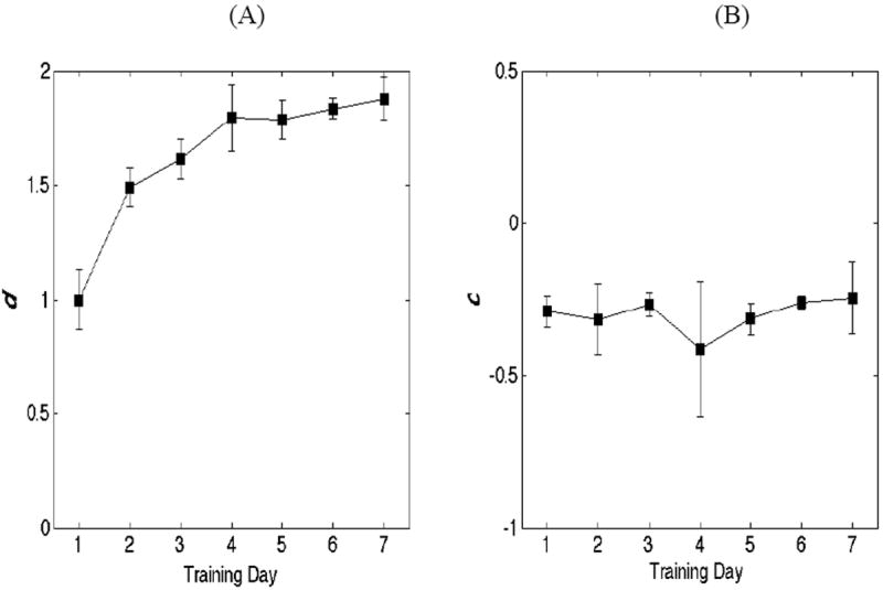
The left panel (A) shows d’ averaged across observers, as a function of learning. The results strongly indicate an overall increase in discriminability across days, with the largest increase occurring between days 1 and 2. The error bars indicate 1 standard error of the mean. The panel on the right (B) shows c (criteria) as a function of learning. Interestingly, the results fail to reveal a pattern between training day and response criteria.

Next, figure 3 shows plots of the log integrated hazard functions for each of the four observers, with each function corresponding to a separate day of training. One may readily observe from the plots in Figure 3 that that the integrated hazard functions within each observer are generally proportional. This suggests that the assumption of proportionality is reasonable in our data.

Figure 3.

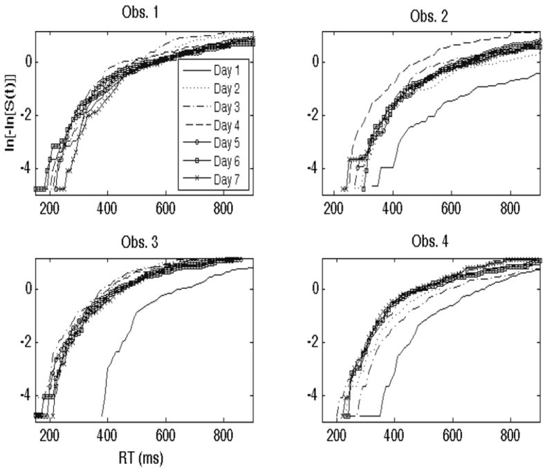
This figure displays the log integrated hazard functions, ln[-ln[S(t)]] or ln[H(t)], across each training day for each of the four observers. As one may observe, the functions are proportional to one another, and for participants 2-4, increase as learning occurs.

An inspection of the data in Figure 3 indicates that a significant amount of learning occurred in observers 2, 3 and 4 across days. This is reflected by the fact that the ln[-ln[S(t)]] functions increased—a finding associated with increased capacity and learning, and therefore faster RTs. In participants 2, 3, and 4, the most notable increase in capacity was observed immediately after the first day of training and one day of consolidation. In participant 4, it appears that learning occurred more gradually, with capacity increasing somewhat steadily at least up until the 4^th or 5^th day. The proportion of log integrated hazard functions in participant 3, interestingly, suggest an increase in capacity from day 1 to day 2, but minimal learning in regards to enhanced efficiency from day 2 onward.

Participant 1 appears to be the only participant that failed to show observable evidence for learning in terms of capacity. The log integrated hazard functions, while showing evidence for proportionality across days, failed to show evidence for increased capacity as a function of training day. In fact, this participant’s integrated hazard ratios appear to show evidence for a slowdown across days. While this participant’s capacity data may be difficult to interpret, it may show evidence for a speed-accuracy trade-off such that the participant slowed down in order to achieve higher accuracy. An analysis of the hits and false alarms for this participant in Table 1 indicate that this may be the case. Participant 1’s d’ on day 1 was .97 (p(Hit) = .82, p(FA) = .48) while on day 7 it was 2.10 (p(Hit) = .94, p(FA) = .29).

In order to statistically test for hazard function orderings, we applied the fixed effect partial likelihood model using day number as a predictor. We also used accuracy as a predictor to determine whether evidence for speed-accuracy trade-offs might emerge. In this particular example, faster RTs and hence greater capacity would come at the expense of accuracy, perhaps due to the lowering of one’s (“yes”) response criteria. The data shown in Table 2 and Figure 3 do not indicate the presence of criteria shifts or this type of speed-accuracy tradeoff for either the group or in any individual observer.

The results of the statistical analyses show, consistent with our predictions, that “day number” was a significant predictor. The beta value, β, was positive for participants 2, 3, and 4, indicating that hazard functions tended to increase as the days progressed (h₂(t) > h₁(t)). The results in Table 3A show that the p-values from the z-test indicate that the results were significant at the .05 level for each participant. Interestingly, the estimated β parameter was negative for participant 1, indicating a slight slow-down as the days progressed. Viewed in conjunction with this observer’s accuracy data, it appears to indicate that the participant decreased their response speed in order to yield an increase in accuracy. However, the criterion change (computed using Table 2) from day 1 to day 7 in this participant was minimal (c = -.43 on day 1; c = -.50 on day 7). This is consistent with the reasoning that participant 1 became more sensitive to detecting the audiovisual association across training, but at the cost of decreased capacity or overall efficiency. Finally, to test whether a significant increase in capacity co-occurred with the increase in d’, we carried out a contrast on mean capacity values from day 1 to day 2. The results from the paired samples t-tests indicated a significant increase in capacity (t(6) = 2.54, p = .043).

Table 3.

A: This table shows results from the Cox Proportional Hazard model fits with “training day” as the predictor for each observer. A positive Beta value (and significant z value) signifies that capacity increased across training days.

Obs.	Beta	z(p)	SE
1	-.04	-1.97 (.05)	.02
2	.13	7.98 (.0001)	.02
3	.05	3.20 (.014)	.02
4	.11	6.50 (.0001)	.02

B: This table shows results from the Cox Proportional Hazard model fits with “accuracy” as the predictor for each observer. A positive Beta value (and significant z value) signifies higher capacity, or a greater amount of work completed, for accurate responses compared to inaccurate responses.
Obs.	Beta	z(p)	SE
1	.16	1.45 (.15)	.11
2	.43	4.40 (.0001)	.10
3	.37	4.00 (.0001)	.09
4	.36	3.47 (.001)	.10

The results in Table 3B show the numerical value for the estimated parameter, β associated with accuracy. We carried out these analyses by coding incorrect responses as 0 and correct responses as 1. A positive value for the β parameter indicates that hazard functions across correct responses were larger than the hazard functions computed for incorrect responses. Crucially, a positive value signifies that observers were responding more accurately and faster to auditory and visual stimuli with matched frequency patterns. Conversely, a negative β value (coupled with evidence for increased capacity in Figure 3 and Table 3A) could indicate that observers actually responded faster when they are incorrect compared to when they are correct. Such a scenario would suggest a very low response threshold leading to fast incorrect responses (e.g., incorrectly saying “no” to signals that match). It is therefore possible for capacity to increase across days without the observer adopting an efficient enough response strategy to slow down when they are incorrect (e.g., Townsend and Altieri, 2012). Hence, fast incorrect responses may actually indicate inefficient performance. The results in Table 3B reveal that each participant showed evidence for a positive β value, although participant 1’s only reached marginal significance. This indicates either that observers set an efficient response criterion, that observers were generally more sensitive to “matched” versus mismatched items, or a combination of the two.

In summary, the behavioral results indicate the presence of multisensory learning by showing an increase in accuracy and sensitivity across days, and a corresponding increase in capacity in three out of four observers. Even the observer that failed to show an increase in capacity exhibited a pattern of results consistent with improved efficiency; a slowing down of processing in conjunction with an increase in capacity.

The major aim of this study was to connect behavioral measures of capacity with neural measures of processing efficiency as measured using EEG. We first predicted that behavior would be correlated with neural changes in which the peak amplitudes of the GFP elicited by the matched signals (i.e., the “yes” responses) would decrease relative to the cases in which the auditory and visual signals were “mismatched”. This pattern of results should emerge since the expenditure of energy necessary for distinguishing these signals should decrease across learning.

Neural Measures of Learning: Mean Global Field Power

The question here deals with how changes in the neural signals co-vary with increases in capacity. We predict an overall reduction in the difference in the EEG signal between the AV_Match and AV_Mismatch conditions. The reason is that as capacity increases, fewer neural resources should be expended to identify congruent versus incongruent signals. Figure 4 shows color-coded plots of the mean GFP separately for each of the four participants on each training day. The left panel shows the mean GFP for the AV_Match condition, and the right panel shows the GFP for the mismatch condition. The panels shows GFP summarized over the time interval of 0-500 ms. Qualitatively, one can observe a reduction in GFP peak amplitude (uV) across the training days for participants 2-4; this difference is most noticeable between day 1, and the other 6 days combined.

Figure 4.

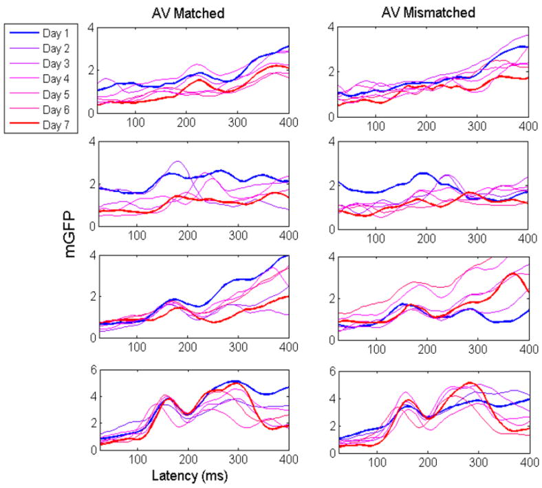
Each panel plots the mean GFP separately for each training day. The panels in the column on the left show the mean GFP for the audiovisual matched trials, and the panels on the right show the mean GFP for the mismatched trials. The top row shows participant 1’s GFP data, the second row participant 2’s, the third row participant 3’s, and the fourth row, participant 4’s.

First, participant 1’s results indicate a noticeable amplitude reduction occurring between days 1 and 3, as expected. However, the difference in amplitude reduction failed to persist. Overall, the magnitude of participant 1’s changes was weak compared to the other participants, which incidentally, mirrors the lack of a positive capacity change.

Next, for participant 2, observable differences began to emerge by the second and third day of training. The observed amplitude reduction appeared across earlier (e.g., 100-200 ms) and later processing times (post 300 ms). As predicted, the changes in neural processing corresponded to the changes in capacity, and persisted over the entire period of seven days. A similar pattern of results may be observed from participant 3’s GFP. However, the changes did not appear to remain stable until the fourth day of learning. Once again, the changes persisted over the course of 7 days, reflecting the corresponding increase in capacity over the same time period. Participant 4 also showed significant evidence for learning-associated neural changes within the first 2-3 days of training. As with participants 2, 3, and 4, the observed changes persisted over a course of 7 days, and generally, corresponded with the increase in capacity that occurred over this period.

To summarize the aforementioned analyses, the bar graph in Figure 5 depicts the mean GFP difference averaged across the interval from 250-350 post-onset for each participant across day of learning. This figure reveals that the activation of the AV_Match (‘yes’) trials was reduced relative to the AV_mismatch (‘no’) trials over this time span (with the exception of participant 1). This observation was tested statistically by carrying out a repeated-measures ANOVA using training day (7) as the within-subject factor. For each day, the average GFP was obtained for a given participant over the interval of 250-350 ms (when effects corresponding to categorization would likely emerge; i.e., P300). Hence, we obtained the average ERP in the time interval from 250-350 ms post stimulus onset and subtracted the amplitude of the AV_Mismatch from the AV_Match condition. The results from the repeated measures ANOVA confirm that there was a significant effect for training day, with the difference between AV_Match and AV_Mismatch becoming smaller (F(6, 18) = 3.91, p = .01). In order to test for baseline effects we carried out a second repeated measures ANOVA with training day again as the within subject factor. We computed the average GFP difference over the time interval from 0-100 ms post stimulus onset for each training day. As expected, a significant effect of training day was not observed for this time interval (F(6, 18) = 1.66, p = .19).

Figure 5.

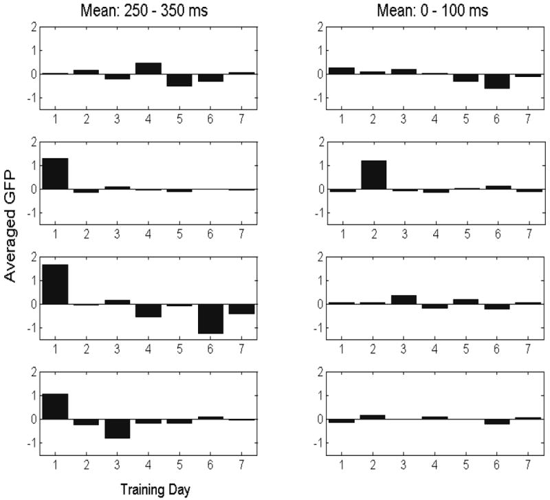
This bar graph shows mean GFP as a function of training day for each participant (rows 1-4; see Figure 4). The panels in the left column show mean GFP averaged over the interval ranging from 250-350 ms post stimulus onset, while the panels in the right column show the mean GFP averaged over the 0-100 ms interval.

Next, we carried out analyses of covariance (ANCOVAs) on each individual participant to test whether GFP values significantly change across days and co-vary with the mean capacity value obtained on that given day. The results for each participant are displayed in Table 4. The results for participants 2, 3 and 4 were significant, indicating that GFP values change across days and significantly co-vary with capacity. Participant 1, however, only showed evidence for marginal significance.

Table 4.

Results from the individual participant ANCOVAs. Capacity was associated with mean GFP across each training day separately for each participant. Calculated F statistics, corresponding p-values, and mean squared error are displayed.

Participant	F	p-value	Mean Sq. Error
1	4.00	.101	.04
2	9.98	.025*	.11
3	8.40	.033*	.30
4	12.43	.017*	.09

^*indicates significance at the alpha level of .05. The df error was equal to 5.

As one final caveat, one alternative explanation for the EEG findings maybe that the reason the neural activity changes across days is because participants actually learned the mismatched stimuli. While this explanation potentially carries some weight, it appears less likely than the former scenario because of the larger number of configurations of mismatched stimuli presented to the participant. Participants have only six matched stimuli that they needed to learn, but thirty mismatched pairs. Furthermore, the task required them to make a “yes” response when they matched—likely biasing participants to focus on learning the matched pairs. We therefore argue that the learning of the “matched” pairs facilitated underlying neural and behavioral changes. To summarize, a viable interpretation of these results is that capacity may constitute a behavioral index of neural efficiency. A correspondence between capacity and GFP was observed, indicating that changes in brain signals during multisensory learning can be interpretable within the milieu of model based capacity measures.

Discussion

Our results show that capacity (e.g., Townsend and Ashby, 1978; Wenger and Gibson, 2004), implemented by utilizing the statistical tools of hazard functions constitutes an appropriate and comprehensive measure of multisensory learning. The methodology of using completion times along with additional measures such as accuracy, d’, and electrophysiological signals, is advantageous in that it provides a multimodal and theoretically based conceptualization of learning. In this framework, observers should show evidence for more efficient resource expenditure in their completion times as learning unfolds. Our study went one step further by providing neurophysiological evidence showing corresponding changes in brain signals consistent with changes in efficiency.

These hazard function based tools were used to assess and quantify multisensory learning over a relatively short time period. The results revealed that each of the participants exhibited at least some evidence of learning, although participant 1’s results significantly diverged from the others. Participant 1 showed the predicted increase in accuracy and sensitivity (d’) across days, without showing marked changes in response bias (c). However, this participant failed to show evidence for increased capacity/efficiency across time—in fact, evidence for decreased capacity (i.e., slowing) was observed. It is possible that this particular strategy was undertaken in order to achieve higher accuracy without a corresponding increase in capacity. This observation is further exemplified by this participant’s GFP in the EEG signals, which failed to provide evidence for a reduction in energy.

The results for participants 2, 3, and 4 showed that capacity increased dramatically within the first few days. These results appeared to be accompanied by an increase in efficient energy expenditure in the brain. In this case, the difference between the GFP amplitude from the matched versus mismatched trials decreased (showing that less processing resources were required to distinguish the signals) as capacity and d’ increased. We interpreted these results as evidence showing that the brain can efficiently learn to associate arbitrary, but spatially and temporally congruent, auditory and visual stimuli. Our data are consistent with the finding that perception is inherently multisensory, and that neural plasticity persists into adulthood with the propensity to effectively learn associations between congruent multimodal events (e.g., Murray et al., 2004; Shams and Seitz, 2008; Seitz, Kim, and Shams, 2006; Thelen, Cappe, & Murray, 2012; Thelen & Murray, 2013). Our approach effectively builds on previous investigations using accuracy as a measure of learning (e.g., Seitz et al., 2006) by quantifying learning in terms of the biologically and neurologically plausible construct of capacity. Current attempts focus on building upon the capacity approach by utilizing both RTs and accuracy in a single function to assess performance relative to independent model predictions (Townsend and Altieri, 2012).

The approach of using combined behavioral and neural assessments of learning have implications regarding how sensory and cognitive experience contributes to our ability to associate multisensory stimuli from the environment. Some important statistical considerations for multisensory binding include whether the signal course originates from a common spatial location (Meredith and Stein, 1986), and also whether the timing between the events are structured in such a way that they appear to originate from a common source (Colonius and Diederich, 2004; Diederich and Colonius, 2009; Powers et al., 2009). For instance, perceptual training on multisensory stimuli narrows the binding window (Powers et al., 2009). These findings indicate that multisensory learning is associated with an increased aptitude for detecting a mismatch, or interpreting auditory and visual signals as originating from separate events. This interpretation bolsters the hypothesis that connections between auditory and visual brain regions are reweighed and strengthened during critical stages of development (e.g., Wallace et al., 2006) and that these connections retain a considerable degree of plasticity throughout adulthood (e.g., Powers et al., 2009).

The findings from Figures 4 and 5 showing the emergence of differences in matched versus mismatched GFP subsequent to100 ms are consistent with observations of interactions between sensory streams in different brain regions (Molholm, Ritter, Murray, Javitt, Schroeder, Foxe, 2002; Naue et al., 2009; Pilling, 2009; van Wassenhove, Grant, & Poeppel, 2005). Brain areas identified as multisensory processing circuits have implicated numerous regions—even early sensory and cortical areas, to association areas such as the STS (e.g., Stevenson and James, 2009; Cappe et al., 2010). Crucially, perceptual, sensory, and developmental experience shapes these connections, and individual differences may well be observed (Powers et al., 2009). This may include the ability to construct associations between qualitatively different signals. Differences in the data patterns suggest unique strategies exploited by different participants. Participant 1, for instance, showed minimal change in GFP and no increase in capacity across training days. This participant did show evidence for an increase in sensitivity (d’), although it seemed to have occurred at the expense of speed and therefore efficiency. Future studies may examine the extent to which multisensory learning, as measured by capacity, is long lasting by examining the extent to which changes persist over a longer period of weeks or months.

Finally, one advantageous feature of the combined capacity and neural analyses concerns the sensitivity for detecting individual differences that may have otherwise not been detected by changes in accuracy alone. Recall that in our data sets, each participant, and the data collapsed across observers, showed evidence for increased accuracy and sensitivity across days. The RT and capacity analysis, intriguingly, revealed individual differences in multisensory learning in young, healthy participants that would otherwise have been missed if we only assessed changes in mean accuracy or RT. The approach for assessing capacity should be extended to assess multisensory processing in clinical populations, such as those with impairments in vision or hearing (Erber, 2003), schizophrenics (Neufeld, Townsend, and Jette, 2007), and in those with autism spectrum disorders (ASDs) (Johnson, Blaha, Houpt, and Townsend, 2010). Future research on multisensory learning may uncover evidence for similar facilitatory cross-modal mechanisms in audiovisual recognition.

References

- Allison PD. Fixed-effects partial likelihood for repeated events. Sociological methods and research. 1996;25:2207–222. [Google Scholar]
- Altieri N, Townsend JT. An assessment of behavioral dynamic information processing measures in audiovisual speech perception. Frontiers in Psychology. 2011;2(238):1–15. doi: 10.3389/fpsyg.2011.00238. [DOI] [PMC free article] [PubMed] [Google Scholar]
- Atkinson RC, Shiffrin RM. Human memory: A proposed system and its control processes. In: Spence KW, Spence JT, editors. The psychology of learning and motivation. Vol. 2. New York: Academic Press; 1968. pp. 89–195. [Google Scholar]
- Beauchamp MS, Lee KE, Argall BD, Martin A. Integration of auditory and visual information about objects in superior temporal sulcus. Neuron. 2004;41(5):809–823. doi: 10.1016/s0896-6273(04)00070-4. [DOI] [PubMed] [Google Scholar]
- Belardinelli MO, Sestieri C, Di Matteo R, Delogu F, Del Gratta C, Ferretti A, et al. Audio-visual crossmodal interactions in environmental perception: an fMRI investigation. Cognitive Processing. 2004;5(3):167–174. [Google Scholar]
- Bernstein LE, Auer ET, Wagner M, Ponton CW. Spatiotemporal dynamics of audiovisual speech processing. Neuroimage. 2008;39(1):423–435. doi: 10.1016/j.neuroimage.2007.08.035. [DOI] [PMC free article] [PubMed] [Google Scholar]
- Calvert GA, Campbell R, Brammer MJ. Evidence from functional magnetic resonance imaging of crossmodal binding in the human heteromodal cortex. Curr Biol. 2000;10(11):649–657. doi: 10.1016/s0960-9822(00)00513-3. [DOI] [PubMed] [Google Scholar]
- Cappe C, Thut G, Romei V, Murray MM. Auditory-visual multisensory interactions in humans: timing, topography, directionality, and sources. Journal of Neuroscience. 2010;30(38):12572–80. doi: 10.1523/JNEUROSCI.1099-10.2010. [DOI] [PMC free article] [PubMed] [Google Scholar]
- Colonius H, Diederich A. The optimal time window of visual-auditory integration: a reaction time analysis. Front Integr Neurosci. 2010;4:11. doi: 10.3389/fnint.2010.00011. [DOI] [PMC free article] [PubMed] [Google Scholar]
- Colonius H, Diederich A. Multisensory interaction in saccadic reaction time: A time-window-of-integration model. Journal of Cognitive Neuroscience. 2004;16(6):1000–1009. doi: 10.1162/0898929041502733. [DOI] [PubMed] [Google Scholar]
- Conrey B, Pisoni DB. Auditory-visual speech perception and synchrony detection for speech and nonspeech signals. J Acoust Soc Am. 2006;119(6):4065–4073. doi: 10.1121/1.2195091. [DOI] [PMC free article] [PubMed] [Google Scholar]
- Cowan N, Elliott EM, Saults JS, Morey CC, Mattox S, Hismjatullina A, Conway ARA. On the capacity of attention: Its estimation and its role in working memory and cognitive aptitudes. Cognitive Psychology. 2005;51:42–100. doi: 10.1016/j.cogpsych.2004.12.001. [DOI] [PMC free article] [PubMed] [Google Scholar]
- Cox DR. Regresion models and life tables. Journal of the Royal Statistical Society, Series B. 1972;34:187–220. with discussion. [Google Scholar]
- Diederich A, Colonius H. Crossmodal interaction in speeded responses: Time window of integration model. In: Raab M, et al., editors. Progress in Brain Research. Vol. 174. 2009. pp. 119–135. [DOI] [PubMed] [Google Scholar]
- Diederich A, Colonius H. Bimodal and trimodal multisensory enhancement: effects of stimulus onset and intensity on reaction time. Percept Psychophys. 2004;66(8):1388–1404. doi: 10.3758/bf03195006. [DOI] [PubMed] [Google Scholar]
- Dixon NF, Spitz L. The detection of auditory visual desynchrony. Perception. 1980;9(6):719–721. doi: 10.1068/p090719. [DOI] [PubMed] [Google Scholar]
- Doehrmann O, Naumer MJ. Semantics and the multisensory brain: how meaning modulates processes of audio-visual integration. Brain Res. 2008;1242:136–150. doi: 10.1016/j.brainres.2008.03.071. [DOI] [PubMed] [Google Scholar]
- Dosher B, Lu ZL. Mechanisms of perceptual learning. Vision Research. 1999;39:3197–3221. doi: 10.1016/s0042-6989(99)00059-0. [DOI] [PubMed] [Google Scholar]
- Fiebelkorn IC, Foxe JJ, Schwartz TH, Molholm S. Staying within the lines: the formation of visuospatial boundaries influences multisensory feature integration. Eur J Neurosci. 2010;31(10):1737–1743. doi: 10.1111/j.1460-9568.2010.07196.x. [DOI] [PubMed] [Google Scholar]
- Frens MA, Van Opstal AJ, Van der Willigen RF. Spatial and temporal factors determine auditory-visual interactions in human saccadic eye movements. Percept Psychophys. 1995;57(6):802–816. doi: 10.3758/bf03206796. [DOI] [PubMed] [Google Scholar]
- Hecht D, Reiner M, Karni A. Multisensory enhancement: gains in choice and in simple response times. Exp Brain Res. 2008;189(2):133–143. doi: 10.1007/s00221-008-1410-0. [DOI] [PubMed] [Google Scholar]
- Hein G, Doehrmann O, Muller NG, Kaiser J, Muckli L, Naumer MJ. Object familiarity and semantic congruency modulate responses in cortical audiovisual integration areas. J Neurosci. 2007;27(30):7881–7887. doi: 10.1523/JNEUROSCI.1740-07.2007. [DOI] [PMC free article] [PubMed] [Google Scholar]
- Hershenson M. Reaction time as a measure of intersensory facilitation. J Exp Psychol. 1962;63:289–293. doi: 10.1037/h0039516. [DOI] [PubMed] [Google Scholar]
- Hillock AR, Powers AR, Wallace MT. Binding of sights and sounds: age-related changes in multisensory temporal processing. Neuropsychologia. 2011;49(3):461–467. doi: 10.1016/j.neuropsychologia.2010.11.041. [DOI] [PMC free article] [PubMed] [Google Scholar]
- James W. The Principles of Psychology. Boston, MA: Harvard University Press; 1890. [Google Scholar]
- James TW, Stevenson RA. The use of fMRI to assess multisensory integration. In: Wallace MH, Murray MM, editors. Frontiers in the Neural Basis of Multisensory Processes. London: Taylor & Francis; 2012. [PubMed] [Google Scholar]
- James TW, Stevenson RA, Kim S. Inverse effectiveness in multisensory processing. In: Stein BE, editor. The New Handbook of Multisensory Processes. Cambridge, MA: MIT Press; 2012. [Google Scholar]
- James TW, VanDerKlok RM, Stevenson RA, James KH. Multisensory perception of action in posterior temporal and parietal cortices. Neuropsychologia. 2011;49(1):108–114. doi: 10.1016/j.neuropsychologia.2010.10.030. [DOI] [PMC free article] [PubMed] [Google Scholar]
- Johnson SA, Blaha LM, Houpt JW, Townsend JT. Systems Factorial Technology provides new insights on global-local information processing in autism spectrum disorders. Journal of Mathematical Psychology. 2010;54:53–72. doi: 10.1016/j.jmp.2009.06.006. [DOI] [PMC free article] [PubMed] [Google Scholar]
- Keetels M, Vroomen J. The role of spatial disparity and hemifields in audio-visual temporal order judgments. Exp Brain Res. 2005;167(4):635–640. doi: 10.1007/s00221-005-0067-1. [DOI] [PubMed] [Google Scholar]
- Kim S, James TW. Enhanced effectiveness in visuo-haptic object-selective brain regions with increasing stimulus salience. Hum Brain Mapp. 2010;31(5):678–693. doi: 10.1002/hbm.20897. [DOI] [PMC free article] [PubMed] [Google Scholar]
- Kim S, Stevenson RA, James TW. Visuo-haptic neuronal convergence demonstrated with an inversely effective pattern of BOLD activation. Journal of Cognitive Neuroscience. 2012 doi: 10.1162/jocn_a_00176. [DOI] [PubMed] [Google Scholar]
- Laurienti PJ, Wallace MT, Maldjian JA, Susi CM, Stein BE, Burdette JH. Cross-modal sensory processing in the anterior cingulate and medial prefrontal cortices. Hum Brain Mapp. 2003;19(4):213–223. doi: 10.1002/hbm.10112. [DOI] [PMC free article] [PubMed] [Google Scholar]
- Lovelace CT, Stein BE, Wallace MT. An irrelevant light enhances auditory detection in humans: a psychophysical analysis of multisensory integration in stimulus detection. Brain Res Cogn Brain Res. 2003;17(2):447–453. doi: 10.1016/s0926-6410(03)00160-5. [DOI] [PubMed] [Google Scholar]
- Luce RD. Response Times: Their Role in Inferring Elementary Mental Organization. Oxford University Press; New York: 1986. [Google Scholar]
- Macaluso E, George N, Dolan R, Spence C, Driver J. Spatial and temporal factors during processing of audiovisual speech: a PET study. Neuroimage. 2004;21(2):725–732. doi: 10.1016/j.neuroimage.2003.09.049. [DOI] [PubMed] [Google Scholar]
- Meredith MA, Nemitz JW, Stein BE. Determinants of multisensory integration in superior colliculus neurons. I. Temporal factors. J Neurosci. 1987;7(10):3215–3229. doi: 10.1523/JNEUROSCI.07-10-03215.1987. [DOI] [PMC free article] [PubMed] [Google Scholar]
- Miller LM, D’Esposito M. Perceptual fusion and stimulus coincidence in the cross-modal integration of speech. J Neurosci. 2005;25(25):5884–5893. doi: 10.1523/JNEUROSCI.0896-05.2005. [DOI] [PMC free article] [PubMed] [Google Scholar]
- McGurk H, Macdonald J. Hearing lips and seeing voices. Nature. 1976;264:746–748. doi: 10.1038/264746a0. [DOI] [PubMed] [Google Scholar]
- McKee SP, Westheimer G. Improvement in vernier acuity with practice. Perception and Psychophysics. 1978;24:258–262. doi: 10.3758/bf03206097. [DOI] [PubMed] [Google Scholar]
- Meredith MA, Stein BE. Spatial factors determine the activity of multisensory neurons in cat superior colliculus. Brain Res. 1986a;365(2):350–354. doi: 10.1016/0006-8993(86)91648-3. [DOI] [PubMed] [Google Scholar]
- Meredith MA, Stein BE. Visual, auditory, and somatosensory convergence on cells in superior colliculus results in multisensory integration. J Neurophysiol. 1986b;56(3):640–662. doi: 10.1152/jn.1986.56.3.640. [DOI] [PubMed] [Google Scholar]
- Meredith MA, Stein BE. Spatial determinants of multisensory integration in cat superior colliculus neurons. J Neurophysiol. 1996;75(5):1843–1857. doi: 10.1152/jn.1996.75.5.1843. [DOI] [PubMed] [Google Scholar]
- Miller LM, D’Esposito M. Perceptual fusion and stimulus coincidence in the cross-modal integration of speech. The Journal of Neuroscience. 2005;25:5884–5893. doi: 10.1523/JNEUROSCI.0896-05.2005. [DOI] [PMC free article] [PubMed] [Google Scholar]
- Molholm S, Ritter W, Murray M, Javitt DC, Schroeder CE, Foxe JJ. Multisensory auditory-visual interactions during early sensory processing in humans: a high-density electrical mapping study. Cognitive Brain Research. 2002;14:115–128. doi: 10.1016/s0926-6410(02)00066-6. [DOI] [PubMed] [Google Scholar]
- Mordkoff JT, Yantis S. An interactive race model of divided attention. Journal of Experimental Psychology: Human Perception and Performance. 1991;17:520–538. doi: 10.1037//0096-1523.17.2.520. [DOI] [PubMed] [Google Scholar]
- Munhall K, Vatikiotis-Bateson E. Spatial and Temporal Constraints on Audiovisual Speech Perception. In: Calvert G, Spence C, Stein BE, editors. The Handbook of Multisensory Processes. Cambridge, MA: MIT Press; 2004. pp. 177–188. [Google Scholar]
- Murray MM, Michel CM, Grave de Peralta R, Ortigue S, Brunet D, Andino SG, Schnider A. Rapid discrimination of visual and multisensory memories revealed by electrical neuroimaging. Neuroimage. 2004;21:125–35. doi: 10.1016/j.neuroimage.2003.09.035. [DOI] [PubMed] [Google Scholar]
- Naue N, Rach S, Strüber D, Huster RJ, Zaehle T, Körner U, Herrmann CS. Auditory event-related responses in visual cortex modulates subsequent visual responses in humans. The Journal of Neuroscience. 2011;31(21):7729–7736. doi: 10.1523/JNEUROSCI.1076-11.2011. [DOI] [PMC free article] [PubMed] [Google Scholar]
- Neufeld RWJ, Townsend JT, Jetté J. Quantitative response time technology for measuring cognitive-processing capacity in clinical studies. In: Neufeld RWJ, editor. Advances in clinical cognitive science: Formal modeling and assessment of processes and symptoms. Washington, D.C.: American Psychological Association; 2007. [Google Scholar]
- Noppeney U, Josephs O, Hocking J, Price CJ, Friston KJ. The effect of prior visual information on recognition of speech and sounds. Cereb Cortex. 2008;18(3):598–609. doi: 10.1093/cercor/bhm091. [DOI] [PubMed] [Google Scholar]
- Pilling M. Auditory event-related potentials (ERPs) in audiovisual speech perception. Journal of Speech, Language, and Hearing Research. 2009;52:1073–1081. doi: 10.1044/1092-4388(2009/07-0276). [DOI] [PubMed] [Google Scholar]
- Powers AR, 3rd, Hillock AR, Wallace MT. Perceptual training narrows the temporal window of multisensory binding. J Neurosci. 2009;29(39):12265–12274. doi: 10.1523/JNEUROSCI.3501-09.2009. [DOI] [PMC free article] [PubMed] [Google Scholar]
- Raab DH. Statistical facilitation of simple reaction times. Transactions of the National Academy of Sciences. 1962;24:574–590. doi: 10.1111/j.2164-0947.1962.tb01433.x. [DOI] [PubMed] [Google Scholar]
- Skrandies W. Global field power and topographic similarity. Brain Topography. 1990;3:147–41. doi: 10.1007/BF01128870. [DOI] [PubMed] [Google Scholar]
- Stein BE, Wallace MT. Comparisons of cross-modality integration in midbrain and cortex. Prog Brain Res. 1996;112:289–299. doi: 10.1016/s0079-6123(08)63336-1. [DOI] [PubMed] [Google Scholar]
- Stevenson RA, Altieri NA, Kim S, Pisoni DB, James TW. Neural processing of asynchronous audiovisual speech perception. Neuroimage. 2010;49(4):3308–3318. doi: 10.1016/j.neuroimage.2009.12.001. [DOI] [PMC free article] [PubMed] [Google Scholar]
- Stevenson RA, Geoghegan ML, James TW. Superadditive BOLD activation in superior temporal sulcus with threshold non-speech objects. Experimental Brain Research. 2007;179(1):85–95. doi: 10.1007/s00221-006-0770-6. [DOI] [PubMed] [Google Scholar]
- Stevenson RA, James TW. Audiovisual integration in human superior temporal sulcus: Inverse effectiveness and the neural processing of speech and object recognition. Neuroimage. 2009;44(3):1210–1223. doi: 10.1016/j.neuroimage.2008.09.034. [DOI] [PubMed] [Google Scholar]
- Stevenson RA, Kim S, James TW. An additive-factors design to disambiguate neuronal and areal convergence: measuring multisensory interactions between audio, visual, and haptic sensory streams using fMRI. Exp Brain Res. 2009;198(2-3):183–194. doi: 10.1007/s00221-009-1783-8. [DOI] [PubMed] [Google Scholar]
- Stevenson RA, Krueger Fister J, Barnett ZP, Nidiffer AR, Wallace MT. Interactions between the spatial and temporal stimulus factors that influence multisensory integration in human performance. Experimental Brain Research. 2012;219:121–137. doi: 10.1007/s00221-012-3072-1. [DOI] [PMC free article] [PubMed] [Google Scholar]
- Stevenson RA, Wilson MM, Powers AR, Wallace MT. The effects of visual training on multisensory temporal processing. Exp Brain Res. 2013 doi: 10.1007/s00221-012-3387-y. [DOI] [PMC free article] [PubMed] [Google Scholar]
- Stevenson RA, VanDerKlok RM, Pisoni DB, James TW. Discrete neural substrates underlie complementary audiovisual speech integration processes. Neuroimage. 2011;55(3):1339–1345. doi: 10.1016/j.neuroimage.2010.12.063. [DOI] [PMC free article] [PubMed] [Google Scholar]
- Saffran JR, Johnson EK, Aslin RN, Newport EL. Statistical learning of tone sequences by human infants and adults. Cognition. 1999;70:27–52. doi: 10.1016/s0010-0277(98)00075-4. [DOI] [PubMed] [Google Scholar]
- Seitz A, Kim, Van Wassenhove V, Shams M. Simultaneous and Independent Acquisition of Multisensory and Unisensory Associations. Perception. 2007;36:1445–1453. doi: 10.1068/p5843. [DOI] [PubMed] [Google Scholar]
- Seitz A, Kim, Shams M. Sound Facilitates Visual Learning. Current Biology. 2006;16(14):1422–1427. doi: 10.1016/j.cub.2006.05.048. [DOI] [PubMed] [Google Scholar]
- Shams M, Seitz A. Benefits of multisensory learning. Trends in Cognitive Science. 2008;12(11):411–417. doi: 10.1016/j.tics.2008.07.006. [DOI] [PubMed] [Google Scholar]
- Tanabe S, Doi T, Umeda K, Fujita I. Disparity-tuning characteristics of neuronal responses to dynamic random-dot stereograms in macaque visual area V4. J Neurophysiol. 2005;94(4):2683–2699. doi: 10.1152/jn.00319.2005. [DOI] [PubMed] [Google Scholar]
- Taylor KI, Moss HE, Stamatakis EA, Tyler LK. Binding crossmodal object features in perirhinal cortex. Proc Natl Acad Sci U S A. 2006;103(21):8239–8244. doi: 10.1073/pnas.0509704103. [DOI] [PMC free article] [PubMed] [Google Scholar]
- Thelen A, Cappe C, Murray MM. Electrical neuroimaging of memory discrimination based on single-trial multisensory learning. Neuroimage. 2012;62(3):1478–1488. doi: 10.1016/j.neuroimage.2012.05.027. [DOI] [PubMed] [Google Scholar]
- Thelen A, Murray MM. The efficacy of single-trial multisensory memories. Multisensory Research. 2013;26(5) doi: 10.1163/22134808-00002426. [DOI] [PubMed] [Google Scholar]
- Townsend JT. The truth and consequences of ordinal differences in statistical distributions: Toward a theory of hierarchical inference. Psychological Bulletin. 1990;108:551–567. doi: 10.1037/0033-2909.108.3.551. [DOI] [PubMed] [Google Scholar]
- Townsend JT, Altieri NA. An accuracy-response time capacity assessment function that measures performance against standard parallel predictions. Psychological Review. 2012 doi: 10.1037/a0028448. [DOI] [PubMed] [Google Scholar]
- Townsend JT, Ashby FG. Methods of modeling capacity in simple processing systems. In: Castellan J, Restle F, editors. Cognitive Theory. III. Hillsdale, NJ: Erlbaum Associates; 1978. pp. 200–239. [Google Scholar]
- Townsend JT, Nozawa G. Spatio-temporal properties of elementary perception: An investigation of parallel, serial and coactive theories. Journal of Mathematical Psychology. 1995;39:321–360. [Google Scholar]
- Townsend JT, Wenger MJ. A theory of interactive parallel processing: New capacity measures and predictions for a response time inequality series. Psychological Review. 2004;111(4):1003–1035. doi: 10.1037/0033-295X.111.4.1003. [DOI] [PubMed] [Google Scholar]
- Talsma D, Senkowski D, Woldorff MG. Intermodal attention affects the processing of the temporal alignment of audiovisual stimuli. Exp Brain Res. 2009;198(2-3):313–328. doi: 10.1007/s00221-009-1858-6. [DOI] [PMC free article] [PubMed] [Google Scholar]
- van Atteveldt NM, Formisano E, Blomert L, Goebel R. The effect of temporal asynchrony on the multisensory integration of letters and speech sounds. Cereb Cortex. 2007;17(4):962–974. doi: 10.1093/cercor/bhl007. [DOI] [PubMed] [Google Scholar]
- van Wassenhove V, Grant K, Poeppel D. Visual speech speeds up the neural processing of auditory speech. Proceedings of the National Academy of Science U S A. 2005;102:1181–1186. doi: 10.1073/pnas.0408949102. [DOI] [PMC free article] [PubMed] [Google Scholar]
- van Wassenhove V, Grant KW, Poeppel D. Temporal window of integration in auditory-visual speech perception. Neuropsychologia. 2007;45(3):598–607. doi: 10.1016/j.neuropsychologia.2006.01.001. [DOI] [PubMed] [Google Scholar]
- Vroomen J, Keetels M, de Gelder B, Bertelson P. Recalibration of temporal order perception by exposure to audio-visual asynchrony. Cognitive Brain Research. 2004;22:32–35. doi: 10.1016/j.cogbrainres.2004.07.003. [DOI] [PubMed] [Google Scholar]
- Wilkinson LK, Meredith MA, Stein BE. The role of anterior ectosylvian cortex in cross-modality orientation and approach behavior. Exp Brain Res. 1996;112(1):1–10. doi: 10.1007/BF00227172. [DOI] [PubMed] [Google Scholar]
- Wallace MT, Carriere BN, Perrault TJ, Jr, Vaughan JW, Stein BE. The development of cortical multisensory integration. J Neurosci. 2006;26(46):11844–11849. doi: 10.1523/JNEUROSCI.3295-06.2006. [DOI] [PMC free article] [PubMed] [Google Scholar]
- Wallace MT, Roberson GE, Hairston WD, Stein BE, Vaughan JW, Schirillo JA. Unifying multisensory signals across time and space. Exp Brain Res. 2004;158(2):252–258. doi: 10.1007/s00221-004-1899-9. [DOI] [PubMed] [Google Scholar]
- Wallace MT, Wilkinson LK, Stein BE. Representation and integration of multiple sensory inputs in primate superior colliculus. J Neurophysiol. 1996;76(2):1246–1266. doi: 10.1152/jn.1996.76.2.1246. [DOI] [PubMed] [Google Scholar]
- Wenger MJ, Gibson BS. Using hazard functions to assess changes in processing capacity in an attentional cuing paradigm. Journal of Experimental Psychology: Human Perception and Performance. 2004;30:708–719. doi: 10.1037/0096-1523.30.4.708. [DOI] [PubMed] [Google Scholar]
- Wenger MJ, Negash S, Petersen RC, Petersen L. Modeling and estimating recall processing capacity: Sensitivity and diagnostic utility in application to mild cognitive impairment. Journal of Mathematical Psychology. 2010;54:73–89. doi: 10.1016/j.jmp.2009.04.012. [DOI] [PMC free article] [PubMed] [Google Scholar]
- Zampini M, Guest S, Shore DI, Spence C. Audio-visual simultaneity judgments. Percept Psychophys. 2005;67(3):531–544. doi: 10.3758/BF03193329. [DOI] [PubMed] [Google Scholar]