Visual and vestibular perceptual thresholds each demonstrate better precision at specific frequencies and also exhibit optimal integration

Abstract

Prior studies show that visual motion perception is more precise than vestibular motion perception, but it is unclear whether this is universal or the result of specific experimental conditions. We compared visual and vestibular motion precision over a broad range of temporal frequencies by measuring thresholds for vestibular (subject motion in the dark), visual (visual scene motion) or visual-vestibular (subject motion in the light) stimuli. Specifically, thresholds were measured for motion frequencies spanning a two-decade physiological range (0.05-5 Hz) using single-cycle sinusoidal acceleration roll tilt trajectories (i.e., distinguishing left-side down from right-side down). We found that, while visual and vestibular thresholds were broadly similar between 0.05 and 5.0 Hz, each cue is significantly more precise than the other at certain frequencies. Specifically, we found that 1) visual and vestibular thresholds were indistinguishable at 0.05 Hz and 2 Hz (i.e., similarly precise); 2) visual thresholds were lower (i.e., vision more precise) than vestibular thresholds between 0.1 Hz and 1 Hz; and 3) visual thresholds were higher (i.e., vision less precise) than vestibular thresholds above 2 Hz. This shows that vestibular perception can be more precise than visual perception at physiologically relevant frequencies. We also found that sensory integration of visual and vestibular information is consistent with static Bayesian optimal integration of visual-vestibular cues. In contrast with most prior work that degraded or altered sensory cues, we demonstrated static optimal integration using natural cues.

we perceive self-motion with exquisite precision. Prior studies show that visual perception is more precise than vestibular perception when discriminating linear motion (Butler et al. 2010; Fetsch et al. 2009, 2012; Gu et al. 2008; MacNeilage et al. 2010). However, it is unclear whether visual precision is universally better than vestibular precision, or if these findings are the result of specific experimental conditions (e.g., the motion frequency content, where frequency always refers to temporal, not spatial, frequency).

Motor reflexes suggest that vestibular cues can be more salient than visual cues, particularly at high frequencies. Specifically, gaze stability is better for vestibular than visual disturbances at higher frequencies, and vice versa at lower frequencies (Crawford 1964; Paige 1983; Robinson 1977). Similarly, postural stability in patients with vestibular deficits is more affected at high than low frequencies (Bles et al. 1983; Peterka and Benolken 1995). However, higher gain responses do not dictate higher precision. Furthermore, perception need not mimic reflexive findings, as demonstrated by qualitative differences in sensory processing in the vestibulo-ocular reflex (VOR) and vestibular perception (Merfeld et al. 2005a, 2005b). Therefore, we chose to measure perceptual thresholds to assay perceptual precision [as per conventional definitions, precision varies inversely to threshold and is defined as the inverse of variance i.e., 1/σ², and is analogous to reliability (Faisal et al. 2008)].

By determining thresholds as a function of frequency, this study combines two classic approaches, measuring thresholds and assessing dynamics, to study 1) how the relative precision of sensory modalities varies with stimulus frequency; 2) how the brain combines sensory cues; and 3) dynamic neuroperception. Thresholds have helped understand the relative precision of sensory modalities (e.g., Ernst and Banks 2002; Gu et al. 2008), and finding frequency responses generally enhances our understanding of dynamic neuroprocessing (e.g., Angelaki and Yakusheva 2009; Cullen 2011; Merfeld et al. 2005a; Valko et al. 2012). To our knowledge, visual and vestibular thresholds have not previously been compared across frequencies with the same motion axis, methods and subjects.

In this study, we compare the frequency response of the visual and vestibular perceptual systems by measuring thresholds across a broad range (0.05–5 Hz) of physiological motion frequencies. Specifically, we characterized the frequency response of the perceptual systems that discriminate leftward from rightward roll tilt in three conditions: “visual” (stationary subjects watched a rotating visual scene), “vestibular” (subjects rotated in the dark) and “visual-vestibular” (subjects rotated in the light while viewing an earth-stationary scene). We found frequency ranges where vestibular thresholds were lower than visual thresholds, demonstrating that visual precision is not universally better than vestibular precision.

In addition, we used this frequency-response approach to investigate the integration of visual and vestibular tilt cues. Previous threshold studies have reported static Bayesian optimal cue integration for rotation (Jurgens and Becker 2006), translation (Butler et al. 2010; Fetsch et al. 2009, 2010, 2012; Gu et al. 2008), and static roll orientation (Clemens et al. 2011; De Vrijer et al. 2009) but visual-vestibular cue integration using thresholds and dynamic tilt has not been reported. Furthermore, unlike the earlier studies that degraded visual cues (Butler et al. 2010; Fetsch et al. 2009, 2012; Gu et al. 2008) or put two sensory cues in conflict (Butler et al. 2010; Fetsch et al. 2009, 2012; Jurgens and Becker 2006), we used natural cue combinations. We found sensory integration that was consistent with static Bayesian optimal integration.

METHODS AND MATERIALS

General methods mimicked recent studies (Grabherr et al. 2008; Valko et al. 2012). Data collection was divided into two studies. In study A, we measured and compared thresholds between 0.05 Hz and 5 Hz; our primary goal in this study was to compare visual precision with vestibular precision across a broad range of frequencies. In study B, we made more meticulous threshold measurements between 1 and 5 Hz, a frequency range that included frequencies (e.g., 2 Hz) where the visual and vestibular thresholds were similar; our primary goals in study were to test the optimal integration hypothesis and to test the hypothesis that vestibular thresholds were lower than visual thresholds above 2 Hz.

Subjects.

Thirteen healthy volunteers (7 men, 6 women; 36 ± 11 yr) participated. Six subjects participated in study A, and five in study B. One subject withdrew before completing testing. We also omitted a second subject's data because of a large vestibular bias, as was done in a related study (Fetsch et al. 2009). Specifically, we excluded any subject with a visual or vestibular bias ≥50% of threshold (bias calculations are described below). This was done because little is known about bias, and it is unknown how bias and threshold interact, and thus we do not know if thresholds measured in a subject with a large bias are representative of normal. Also, it is unknown how biases affect integration, since a subject with different visual and vestibular biases would presumably be receiving incongruent information from the two cues. In fact, it is worth noting that some (Garcia-Perez and Alcala-Quintana 2013) even question the perceptual origins of such biases, specifically suggesting that such biases include cognitive decision-making biases. All subjects underwent a clinical vestibular diagnostic exam to screen for undiagnosed vestibular disorders, which consisted of Hallpike testing, caloric electronystagmography, angular VOR evoked via rotation and postural control measures. Subjects also answered a questionnaire to indicate any history of dizziness or vertigo; back/neck problems; cardiovascular, neurological and other physical problems; as well as motion sickness susceptibility. Informed consent was obtained from all subjects prior to participation in the study. The study was approved by the local ethics committee and has been performed in accordance with the ethical standards laid down in the 1964 Declaration of Helsinki.

Testing conditions and motion stimuli.

Motion was in roll tilt about a nasooccipital axis through head center at the level of the vestibular organs and was provided by a motion platform (MOOG 6DOF2000E) controlled by a computer in real time.

Each subject was tested in each of three conditions, vestibular, visual or visual-vestibular, during separate sessions. In the vestibular condition, subjects sat on the motion platform and were tilted in roll to the left or right in the dark. In the visual condition, subjects sat in a stationary chair and viewed the roll motion of a visual scene mounted on the motion platform. In the visual-vestibular condition, subjects sat on the motion platform and were tilted in roll while viewing the earth-stationary visual scene. Our vestibular stimuli activated both the semicircular canals (SCC) and otolith organs, providing both motion and displacement cues. Similarly, our visual stimuli provided both motion and displacement cues. Using the same platform to provide motion for the subject or the visual scene ensured that the motion dynamics were matched across conditions.

We desired to determine and compare thresholds that were relevant to real-life, physiological situations, so we chose to make the visual scene as realistic as possible, instead of providing a computer-displayed view. Of course this realism limits our ability to manipulate visual cues experimentally, but realistic visual scenes are likely to provide near-maximal information compared with sinusoidal gratings or random dot patterns. The realistic view (Fig. 1) was dominated by a large poster of a forest and also included other cues typical of our experiment rooms such as a vertical wire bundle. The forest poster (cropped version of “Ashley, Aspens NF” by Alain Thomas, 1.0 m × 0.4 m) was mounted directly in the subject's line of sight and attached 0.05 m in front of the background. The edges of the poster and the trees in the forest provided strong vertical and horizontal cues. The subjects saw the view through a round aperture (0.30 m diameter) made from a block of black plastic placed near the normal visual near point; the peripheral visual scene consisted of a low-contrast black fabric that prevented use of body or motion device landmarks to judge motion of the visual scene (e.g., by visually aligning their knee with an object). In study A, for the visual-vestibular condition, the poster was mounted on the wall of the experiment room and the view also included vertical wire bundles. For all of study B and for the visual condition in study A, the forest poster was mounted on a life-sized realistic print of a photograph of the real wall scene described above that was used in study A for the visual-vestibular condition. The print included the vertical wire bundles, and the forest poster was attached 0.05 m in front of the print. The photograph was taken from the perspective of the subject sitting on the motion platform using a Nikon Digital SLR camera. Two subjects independently reported during visual-only testing that they felt that they were looking at the actual wall of the experiment room and doing the visual-vestibular testing, rather than looking at the large print and doing visual-only testing. This anecdotally suggests that the large print was compelling.

Fig. 1.

A representation of the visual scene used for the “visual” and “visual-vestibular” conditions. The black circular aperture was precisely aligned with the roll rotation axis and placed close to the normal visual near point to help minimize the comparison of body-fixed and space-fixed visual cues. Small differences between the visual scenes in studies A and B are examined in detail in the discussion. The forest poster “Aspens, Ashley NF” is replicated with permission of photographer Alain Thomas.

In study A, the aperture was mounted 0.24 m from the eyes, the view was 1.3 m from the eyes, and the field of view (FOV) was 63°. The forest poster filled more than one-half of the horizontal FOV and one-fourth of the vertical. In study B the aperture was mounted 0.28 m from the eyes, the view was 0.95 m from the eyes and the FOV was 56°. The forest poster filled most of the horizontal FOV and one-third of the vertical. The difference in display and overall FOV between the two studies is not large. More fundamentally, the differences do not affect our conclusions, because we do not compare data across the two studies that also use different subjects. Subjects were instructed to fixate the poster during motion.

We treat vestibular and visual perception as dynamic systems, meaning that the system response depends on both current and past inputs. We used the common approach for characterizing dynamics of measuring responses (i.e., perceptions) to known stimuli at a range of frequencies. Variations in threshold across frequencies indicate different filtering, i.e., that responses to different cues depend on current and past inputs being weighted differently. As with many other motion threshold studies (Benson et al. 1986, 1989; Butler et al. 2010; Crane 2012a; Grabherr et al. 2008; Haburcakova et al. 2012; Kolev et al. 1996; Roditi and Crane 2012a, 2012b; Soyka et al. 2011; Valko et al. 2012; Zupan and Merfeld 2008), motion stimuli were single cycles of sinusoidal acceleration with frequency f. Figure 2 shows the corresponding cosine bell velocity and sigmoidal displacement and demonstrates how the amplitudes of the three co-vary for a given frequency. While not a primary objective of this study, when compared across frequencies, this approach is sometimes used to separate the contributions of position, velocity, acceleration and higher-derivate cues. For example, if visual threshold in peak velocity is relatively constant across a range of frequencies, it suggests that visual perception at those frequencies depends primarily on peak velocity. Alternatively, if threshold in displacement has a slightly negative slope, and threshold in peak velocity has a slightly positive slope, it suggests that visual perception depends primarily on both displacement and velocity cues. It is important to note that crossover points between visual and vestibular cues occur at the same frequencies, regardless of the units in which thresholds are plotted. The equations defining motion are as follows: angular acceleration α(t) = A sin(2πft); angular velocity ω(t) = A/(2πf)[1 − cos(2πft)], and displacement Δθ(t) = A/(2πf)[t − 1/(2πf) sin(2πft)]. Since the same Moog platform was used for both visual and vestibular motion, any displacement infidelity at high frequencies would impact both visual and vestibular thresholds. As in many studies that use sinusoidal motion, we define motion frequency f as the inverse of the period of one cycle, even though strictly frequency is defined only for infinite-duration sinusoids. Fourier analysis demonstrates the consequences of truncating sinusoids to finite durations and shows that, while truncation causes some distortion of frequency content, the practical consequences are small.

Fig. 2.

Examples of ideal motion stimuli for 2 Hz and 5 Hz. Although both have the same peak velocity of 2°/s, they differ in peak velocity and acceleration (A). Actual device position (gray x) from a 60-Hz feedback signal closely matches the theoretical motion. f, frequency; T, period.

We conducted a number of verifications to ensure that actual motion matched desired motion, since mechanical dynamics could result in a mismatch, especially at higher frequencies. Before beginning the studies presented herein, we performed a detailed calibration between 0.01 Hz and 5 Hz using a 6 degree-of-freedom sensor (Analog Devices ADIS16360) attached directly to the Moog platform. This calibration procedure included the application of single-cycle sinusoidal acceleration like those used herein, as well as standard multicycle steady-state sinusoidal oscillations. During this calibration process, we designed a simple first-order compensator to make device motion closer to the desired performance. The compensators had the form (b₁ + b₂z)/(1 + a₂z), where z represents the standard discrete-time z-transform for a Moog 60-Hz update and sampling rate. With this compensation, actual roll tilt motion was within 0.3 dB (i.e., accurate to within 4%) of desired motion at frequencies of 0.01 Hz to 5 Hz. We also investigated whether there were any nonlinearities whereby motion characteristics varied with amplitude and found that our device is capable of producing the desired motions for both small and large displacements (Fig. 3A). We also confirmed that the Moog feedback signal accurately measured motion by independently measuring motion using an accelerometer mounted to the helmet support structure (Fig. 3B). We note that small platform motion errors would affect visual and vestibular conditions equally, so it would not impact the visual-vestibular threshold comparison, which is our primary finding. Another consideration is that, although we used a split helmet “vice” that firmly held the head in roll, it is still possible that inertia would cause the head to slip slightly, resulting in slower head motions during the vestibular condition at high frequencies. This would result in an artifact of higher vestibular thresholds. In contrast, this artifact would be unlikely to affect visual thresholds because of the secure attachment between the visual scene and platform. Thus, if this artifact were occurring and were corrected, it would actually increase the difference between vestibular and visual thresholds at 5 Hz, and thus our primary hypothesis would be more strongly supported. Similar reasoning applies to other artifacts that would result in inflated vestibular thresholds. For example, there is evidence that external “noise” may raise thresholds for nonvestibular perception (e.g., Watamaniuk and Heinen 1999), although a recent study showed that increased device vibration did not significantly change yaw rotation direction recognition thresholds (Chaudhuri et al. 2013).

Fig. 3.

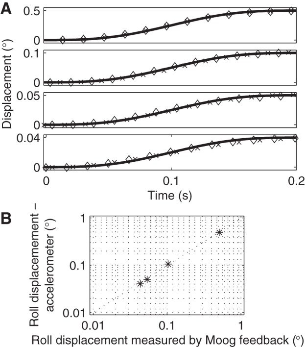
A: actual device position with (◇) and without (x) a human subject closely matches the theoretical motion (line) for various displacement magnitudes. Device position from a 60-Hz Moog position feedback signal is shown. Displacements of 0.04°, 0.05° and 0.10° are shown because they span the thresholds at 5 Hz for the three testing conditions, as well as the displacements for trials at fixed ratios (1.30, 1.55, 1.80) of an initial estimate of threshold. B: an accelerometer used to measure tilt verified that the Moog feedback signal accurately reported device displacement at 5 Hz for motions near threshold and larger.

Experimental procedure.

Subjects were seated upright in a racing-style chair and secured with a five-point harness. The subject's head was fixed relative to the chair and platform with a foam-lined helmet that could be tightened until snug. We attempted to minimize the influence of cues other than visual and vestibular. Wind cues were reduced by covering all skin surfaces (gloves, long sleeves, clear plastic visor over face). Tactile cues were reduced to the extent possible using foam padding. Auditory cues were masked with noise-canceling headphones playing white noise (∼60 dB). Vestibular-only trials were performed in the dark in a light-tight room. Relative success of these techniques to reduce task-relevant cues is demonstrated by elevated thresholds measured in patients suffering total vestibular loss (Valko et al. 2012).

After motion, subjects were required to push a button in their left hand if they perceived leftward motion or a button in their right hand if they perceived rightward motion. Subjects were instructed to make their best guess if they were unsure. Each trial started from upright, and a subthreshold motion returned the platform to upright after each trial. A computerized voice indicated to subjects that motion was commencing (“start”), and that motion was complete and that they needed to respond (“respond”). Before each condition, practice trials spanning a range of stimuli magnitudes were administered to assure that subjects understood the task. For the visual and visual-vestibular conditions, a computer-controlled light turned on 3 s before motion and turned off after the subject responded, and thus the subjects had no visual cues while they moved back to the origin.

For study A, seven frequencies spanning 2 decades, 0.05, 0.1, 0.2, 0.5, 1, 2 and 5 Hz, were tested. Motion magnitudes were selected by an adaptive procedure, a three-down, one-up staircase paradigm (Leek 2001), meaning that stimuli magnitude reduced after three consecutive correct responses, and increased after one incorrect response. Testing started at stimuli magnitudes well above typical thresholds (0.76°/s at 0.05 Hz, 1.53°/s at 0.1 Hz, 3.18°/s at 0.2 Hz, 2.55°/s at 0.5, 1 and 2 Hz, 2.04°/s at 5 Hz). Testing ended after the adaptive track reached the third minimum direction reversal, which occurs when the subject responds incorrectly following at least three correct responses. Each frequency was tested on two separate occasions to reduce measurement error, and thresholds were determined using the pooled data across both blocks. With three conditions this resulted in a total of 42 blocks per subject. On average there were four blocks per test-session. Study A included a total of 9,545 trials for all subjects, with each threshold (i.e., for each subject and frequency, with two blocks combined) based on between 46 and 120 trials, and a mean of 76 trials.

Study B focused on a more narrow range of 1, 2, 3, 4 and 5 Hz. For each frequency, all three conditions were tested on the same day to reduce possible day-to-day variation in thresholds, and subjects were required to take breaks between conditions. For study B, we desired to have lower measurement variability than in study A to be able to test the optimal integration hypothesis. To more precisely measure thresholds, we used a two-stage approach to adaptively select stimuli magnitude. In the first stage, a three-down, one-up staircase, starting at 4°/s, was used. After each trial, a real-time psychometric fit was performed, and the coefficient of variation (CV) of the threshold was computed as a measure of goodness of fit. The first stage ended when CV was less than 0.25. In the second stage, the method of constant stimuli was utilized: testing occurred at three magnitudes that were provided at fixed ratios (1.30, 1.55, 1.80) of the threshold calculated at the end of the first phase, with motion in both directions. These ratios were selected because they tailored the stimuli for each subject to yield a large amount of information for each trial (Wetherill 1963). Testing continued until CV was less than 0.10. Each block had between 183 and 578 trials with a mean of 240 trials per block. Study B included a total of 18,027 trials for all subjects.

Two small supporting studies are described in the discussion. The first measured visual thresholds using the methods described for study A, but tested a single frequency only (1 Hz), and varied the size of the round aperture to test the effects of changing FOV. The second measured visual-vestibular thresholds using the methods described for study A, but compared thresholds with and without the round aperture.

Each frequency was tested in a block of contiguous trials. The order of frequencies and conditions (vestibular, visual, visual-vestibular) was randomized across subjects. In each block, an adaptive one-interval two-alternative categorical forced choice procedure (Leek 2001; Treutwein 1995) was used.

Threshold determination.

Thresholds were determined using a psychometric curve fit. A Gaussian cumulative distribution psychometric function defined by two parameters, sigma and bias, was fit to the data of each block, using a maximum likelihood fit (MATLAB Statistics Toolbox version 7.0) determined using a generalized linear model and probit link function (Haburcakova et al. 2012; Zupan and Merfeld 2008). The Gaussian distribution was chosen (Wichmann and Hill 2001), as in every similar study of which we are aware (e.g., Butler et al. 2010; MacNeilage et al. 2010; Roditi and Crane 2012b; Soyka et al. 2011), because it correctly fits the second-order statistics (i.e., variance of the underlying distribution). Although a logistic distribution may also provide an appropriate fit, the differences between the logistic and Gaussian distributions are small (Dobson and Barnett 2008) and inconsequential, and the most appropriate distribution cannot be determined without extensive data collection. The underlying Gaussian probability distribution is described by “bias,” which represents an offset from zero, and “sigma” which represents the noise standard deviation (Dobson and Barnett 2008; Haburcakova et al. 2012; Merfeld 2011). We report all thresholds as “1-sigma thresholds” i.e., T_σ = σ, which can be converted to the commonly reported 79.4% threshold targeted by a three-down/one-up staircase, using T_79.4% = 0.82σ (Merfeld 2011).

Theoretical framework.

Signal detection theory relates the variability of an underlying noisy sensory estimate to the threshold for perceptual responses (Green and Swets 1966; Merfeld 2011). Figure 4 shows the assumed relationship between sensory stimuli and noisy sensory estimates as defined by a standard deviation σ, which, in the absence of any vestibular bias, equals the stimulus level where 84% of motion directions will be correctly recognized (Green and Swets 1966). In this hypothetical example, vestibular has the largest variability, with σ_vestibular = 1, visual has a slightly lower variability with σ_visual = 0.85, and visual-vestibular has lower variability than either cue individually with a standard deviation σ_{vestibular+visual} = 0.65. Since precision is defined as the inverse of variance, i.e., 1/σ², and since we use 1-sigma thresholds, threshold ${\mathrm{T}}_{\mathrm{\sigma }}\mathrm{=}\mathrm{\sigma }\mathrm{=}\mathrm{1}\mathrm{/}\sqrt{\mathrm{p}\mathrm{r}\mathrm{e}\mathrm{c}\mathrm{i}\mathrm{s}\mathrm{i}\mathrm{o}\mathrm{n}}$. Thus an improvement in precision is indicated by a smaller threshold. The term reliability, used by some related studies, is analogous to precision (Faisal et al. 2008).

Fig. 4.

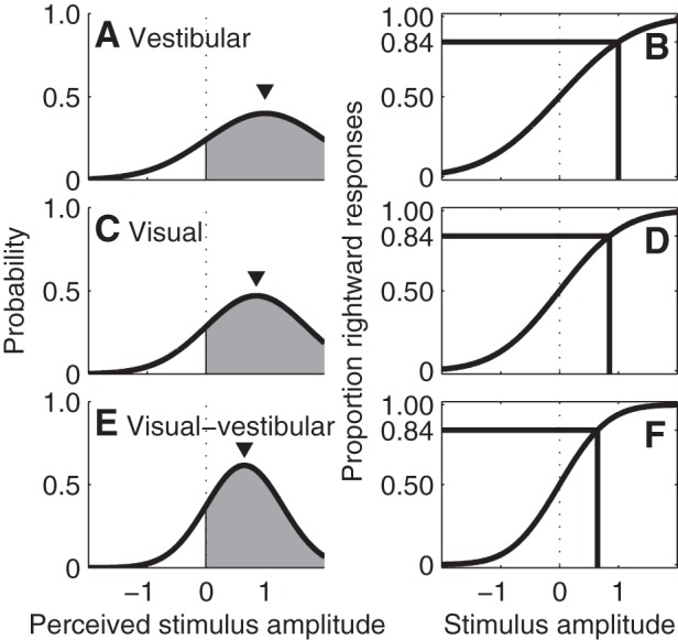
Hypothetical relationships between noise and thresholds. A: vestibular noise has a standard deviation of 1.0, yielding the probability density function (PDF) showing the likely perceived stimulus given an actual stimulus amplitude (▼) of 1.0. The gray area shows the probability the brain will perceive the motion to be rightward (i.e., positive). In this example, the area is 84.1% because the stimulus amplitude equals the noise standard deviation. B: the psychometric function shows the probability that a subject will respond that the motion is rightward, which is equal to the gray area under the PDF when the PDF is centered at that stimulus amplitude. Lines show the threshold, i.e., the stimulus amplitude that leads to 84.1% correct responses, which occurs when the stimulus amplitude equals the noise standard deviation. In these examples no bias is assumed. C and D: PDF and psychometric function, respectively, for a visual input with a standard deviation of 0.85 and stimulus amplitude of 0.85, yielding a lower threshold than for vestibular inputs. E and F: PDF and psychometric function, respectively, for combined visual-vestibular stimulation, assuming that precision improves by having both cues together, which corresponds to a smaller standard deviation than individual cues. The smaller standard deviation corresponds to a narrower PDF and steeper psychometric function.

Bayesian optimal integration results in a sensory estimate that has the highest possible precision for the linear weighting of static individual cues (e.g., Ernst and Banks 2002; Gelb 1992; Gu et al. 2008; Landy et al. 1995). The predicted optimal (e.g., maximum likelihood) integration occurs when the weights are inversely proportional to the precision of each cue, if one assumes that the sensory cues have Gaussian distributions, independent noise sources, and uniform priors. For two cues, the predicted optimal visual-vestibular threshold occurs when the vestibular weight w_vestibular = (1/σ_vestibular²)/(1/σ_vestibular² + 1/σ_visual²) and visual weight w_visual = (1/σ_visual²)/(1/σ_vestibular² + 1/σ_visual²), and can be determined using the relationship (e.g., Ernst and Banks 2002; Gu et al. 2008; Landy et al. 1995): 1/σ̂_{vestibular+visual}² = 1/σ_vestibular² + 1/σ_visual².

The exact same relationship can be derived using minimum-variance unbiased estimation (Gelb 1992). In Fig. 4, we show the psychometric curve for visual-vestibular if it were to follow static optimal weighting, so that

$${\sigma }_{\text{vestibular}+\text{visual}}={\widehat{\sigma }}_{\text{vestibular}+\text{visual}}=\sqrt{\frac{1}{\frac{1}{{1.0}^2}+\frac{1}{{0.85}^2}}}=\mathrm{0.65.}$$

Statistical analysis.

All statistical calculations across subjects were performed after taking the logarithm of the threshold, because population studies have shown that human vestibular thresholds follow a log-normal distribution (Benson et al. 1986, 1989), including means, standard deviations, and tests of statistical significance. For presentation, mean and standard error bars were transformed back to physical units.

After viewing the data, we hypothesized that there was one frequency region in which visual thresholds were lower than vestibular thresholds, and another range in which the opposite was true. To test these hypotheses, comparisons of thresholds in these two conditions across multiple frequencies were performed using an ANOVA with one random factor (subject) and two fixed factors (frequency, condition) that combined the results of study A and study B using an unbalanced design, and used α = 0.05 to reject the null hypothesis. We used a single statistical test for each hypothesis. Therefore, multiple-comparison correction is not applicable.

To determine whether static optimal integration occurred, four hypotheses were tested using planned comparisons to explain how vestibular and visual thresholds combine to give the visual-vestibular thresholds: 1) they depend only on vestibular thresholds, 2) they depend only on visual thresholds, 3) they are the minimum of vestibular or visual thresholds at each frequency, 4) they depend on the linear optimal maximum likelihood estimate for integration of vestibular and visual cues. For each of the hypotheses, a visual-vestibular predicted threshold was determined and compared with the visual-vestibular actual threshold using ANOVA. The optimal integration hypothesis would be supported if the prediction differed significantly from the data for all but the fourth hypothesis.

RESULTS

Figure 5, A–C, shows results for one subject at 5 Hz in the vestibular, visual, and visual-vestibular conditions, respectively. The experimental data show the proportion of trials at each stimulus amplitude in which the subject responded that motion was rightward. In all conditions, when there are large, positive (rightward) motions, the subject selected rightward in close to 100% of trials. When there are large negative (leftward) motions, the subject selected rightward in close to 0% of trials. For tiny motions, the subject selected rightward in close to 50% of trials, indicating that they were guessing. The data are fit by a Gaussian cumulative distribution function to give the psychometric curve fit (black curve). The thresholds σ at the P = 84.1% level are shown with black lines. For this subject and frequency, the threshold is smaller for the vestibular condition (Fig. 5A) than visual condition (Fig. 5B). In this illustrative example, the threshold for the visual-vestibular condition (Fig. 5C) is less than for either visual or vestibular, suggesting that, when the brain has both cues, it recognizes motion direction more precisely.

Fig. 5.

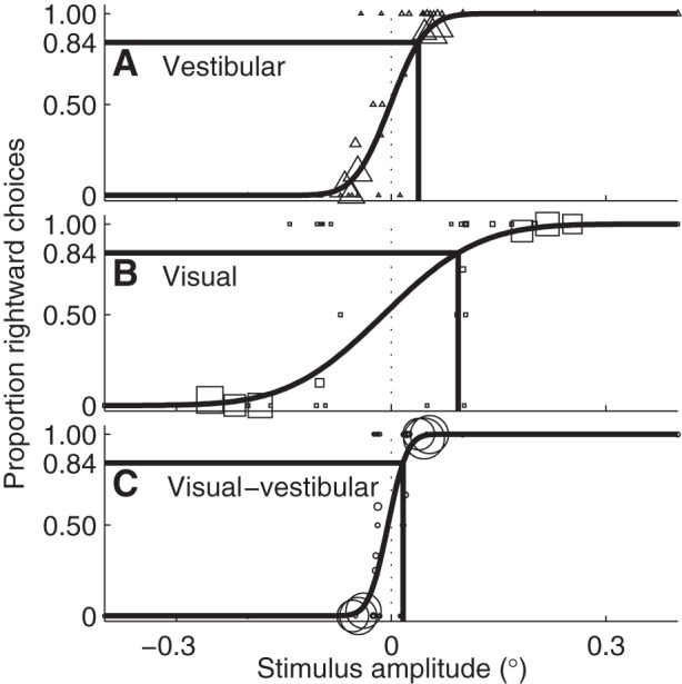
Example of psychometric curves from one subject at 5 Hz. A: the triangles represent the proportion of rightward choices at each stimulus amplitude with vestibular cues. The size of the symbols reflects the number of trials at that amplitude. The psychometric curve is fit to these data, and the black lines indicate the threshold, the place where the stimulus amplitude at which subjects will report rightward motion 84.1% of the time. B and C: the same fits for visual cues (□), and vestibular and visual cues (○), respectively.

Frequency responses of vestibular, visual and visual-vestibular thresholds.

In study A, we measured vestibular, visual and visual-vestibular thresholds over 2 decades of temporal motion frequencies from 0.05 to 5 Hz (Fig. 6A). We plot both displacement (Fig. 6A) and velocity (Fig. 6C) at threshold to show that there are threshold variations in both domains. Each data point is the geometric mean of six subjects. The average vestibular threshold (triangle) is 1.53° at 0.05 Hz, when the motion takes 20 s, meaning that roll tilt direction was on average correctly recognized 84.1% of the time for a displacement of 1.53°. As frequency increases, the displacement threshold decreases, reaching 0.047° at 5 Hz, i.e., a 0.2-s motion. The visual thresholds (squares) also decrease with frequency, decreasing from 1.40° at 0.05 Hz to 0.088° at 5 Hz. Visual-vestibular thresholds (circles) follow the same overall pattern as the individual cues, gradually decreasing from 1.27° at 0.05 Hz to 0.04° at 5 Hz.

Fig. 6.

The frequency response of roll tilt recognition thresholds for vestibular (△), visual (□) and visual-vestibular (○) cues. The predicted visual-vestibular threshold for static optimal integration of individual thresholds is also shown (x's). A and B: displacement thresholds from studies A and B, respectively. Each point is the geometric average across subjects (six in A, five in B), with the bars indicating standard error of the mean. While study A measured across 2 decades of frequency, study B focused on a narrow range of frequencies. For quantitative evaluation, vestibular, visual and visual-vestibular displacement thresholds are presented numerically along the top. Caution is required for direct comparisons of study A and B thresholds because they use different subjects and slightly different methods. C and D: the thresholds in peak velocity, which are most relevant at higher frequencies where velocity cues are more salient.

In study B we made more precise (i.e., more trials, lower variability) measurements (Fig. 6, B and D) at five closely-spaced frequencies (1, 2, 3, 4, 5 Hz) after finding that visual and vestibular thresholds are similar around 2 Hz in study A. Each data point is the geometric mean of five subjects. Vestibular thresholds (triangles) decreased from 0.28° at 1 Hz to 0.040° at 5 Hz. Visual thresholds (squares) decreased more gradually from 0.20° at 1 Hz to 0.072° at 5 Hz. Visual-vestibular thresholds (circles) decreased from 0.16° at 1 Hz to 0.034° at 5 Hz.

Differences in the frequency response of visual and vestibular perceptual thresholds.

We examined the dynamics of vestibular (triangles) and visual (squares) thresholds in both studies A and B (Fig. 6, A and B), and found that:

• 1) Vestibular and visual thresholds are very close at 0.05 Hz.

• 2) There is a cross-over at 2 Hz where vestibular and visual thresholds are very close.

• 3) Vestibular thresholds were lower than visual thresholds above the 2 Hz cross-over (ANOVA, P = 0.0013).

• 4) Visual thresholds were lower than vestibular thresholds for frequencies ranging from 0.1 Hz to 1 Hz (ANOVA, P < 0.001).

Optimal static vestibular-visual integration in roll tilt using two natural cues.

The optimal predictions for the visual-vestibular thresholds (Fig. 6, A and B, dotted lines) were computed based on the individual vestibular and visual thresholds at each frequency. The visual-vestibular thresholds (thin solid lines) closely followed the optimal prediction for visual-vestibular thresholds, suggesting that optimal or near-optimal vestibular-visual integration was occurring. There is not a significant difference between the experimental results and optimal predictions (ANOVA, P = 0.15). To further support the optimal hypothesis, we ruled out three other potential hypotheses. Specifically, we found that the visual-vestibular thresholds were significantly lower than visual thresholds alone (ANOVA, P = 0.005), vestibular thresholds alone (ANOVA, P < 0.001), and the best of these two individual thresholds (ANOVA, P < 0.001).

DISCUSSION

Dynamics of vestibular and visual perceptual thresholds.

To our knowledge, this is the first comparison of vestibular and visual motion perception thresholds across a broad range of frequencies. It shows for the first time that vestibular perceptual thresholds can be lower than visual thresholds for a range of frequencies that we regularly experience and that are behaviorally important. Specifically, we report that: 1) visual and vestibular thresholds were indistinguishable at 0.05 Hz and 2 Hz; 2) visual thresholds were lower than vestibular thresholds for frequencies ranging from 0.1 Hz to 1 Hz; and 3) visual thresholds were higher than vestibular thresholds above 2 Hz. For comparison, previous studies using linear motion found lower visual than vestibular thresholds, except when visual cues were intentionally degraded (Butler et al. 2010; Fetsch et al. 2009, 2012; Gu et al. 2008; MacNeilage et al. 2010). These earlier findings may, in part, be due to the frequency content (∼0.5–1 Hz) of the stimuli; we also found lower visual than vestibular thresholds in this frequency range.

Our findings appear consistent with other relevant studies. Our vestibular thresholds as a function of frequency in the dark are very similar to those recently reported for roll tilt by Valko et al. (2012), and also quite similar to those recently reported by other groups at 2 Hz (Crane 2012b) and for low-velocity tilts using a detection task (Janssen et al. 2011). Another study (Lagace-Nadon et al. 2009) reported that visual roll tilt thresholds decreased with increasing temporal frequency, consistent with our findings. Their thresholds were approximately 8× higher than ours, which can probably be attributed to visual display differences, as we chose to use a broader realistic scene as opposed to their narrower low-spatial-frequency scene. Beyond this, it is difficult to compare vestibular and visual precision using the results of these two studies because they used different subjects and different methods.

Our results complement previous studies reporting frequency-dependent differences between visual and vestibular reflexive responses. For example, gaze stability studies (Crawford 1964; Paige 1983; Robinson 1977) suggest that ocular stability is more vestibular dependent at high frequencies and visual dependent at low frequencies, since these studies report that the VOR gain acts like a high-pass filter, and optokinetic gain as a low-pass filter. Similar findings have been reported for postural stability (Bles et al. 1983; Peterka and Benolken 1995) and when controlling a vehicle (Zacharias and Young 1981). In both reflexes and perception, dynamics originate from the sensory periphery and central processing (as well as motor responses for reflexes), but these dynamics are not necessarily the same. For example, there are qualitative differences in sensory processing between the VOR and vestibular perception (Merfeld et al. 2005a, 2005b), and differences in the frequency response between VOR thresholds and vestibular perceptual thresholds (Haburcakova et al. 2012). In addition, perception usually involves a host of processes, including cognitive, that could be the source of our measured perceptual dynamics and differences between vestibular and visual perceptual precision.

Given the complex nature of visual processing, an important question is how broadly applicable are our findings. For several reasons, we think that our findings are broadly applicable. First, we made additional measurements (Fig. 7) of visual thresholds with different FOVs and found that visual thresholds were relatively invariant over a large range. Specifically, we found a small, but statistically insignificant, increase in visual threshold below 30° FOV. More importantly, there were no consistent threshold variations measured for FOVs between 34° and 63°, which includes the FOVs for the primary studies. Second, since our scene was realistic, the spatial frequencies in our visual scene were, by definition, representative of a typical indoor scene. Third, the physical images used for our visual scene avoided discrete pixel effects associated with digital displays. Finally, we eliminated relative motion cues and/or relative displacement cues, those in which space-fixed and body-fixed landmarks could be readily compared, by using a circular aperture. To demonstrate the importance of eliminating relative visual cues, we measured thresholds without the aperture present (Fig. 8) and found that the thresholds measured without the aperture were 30% lower than with the aperture, which was a significant difference (ANOVA, P = 0.009).

Fig. 7.

Field of view (FOV) above 30° shows little effect on visual thresholds. Although visual thresholds seem to be somewhat higher when FOV was much smaller (20°) than that used in our studies (63° in study A, 56° in study B, as indicated by arrows), none of the differences observed, nor the overall trend, are statistically significant. FOV was modified by changing the diameter of the circular aperture through which subjects viewed the visual scene, as demonstrated in the illustrations (a larger picture of the visual scene appears in Fig. 1). The visual scene was slightly closer in study B than study A, as shown by the larger forest poster size in the illustration, and thus 56° was not sampled for this FOV study. Subjects always viewed the scene binocularly. The stated FOV is for all areas that subjects could see, even if by only one eye, which became challenging at smaller diameters. At 20° FOV, the FOV with binocular coverage was between 3° and 6°, depending on the interpupilliary distance. Each point is the geometric average across four subjects, with the bars indicating standard error of the mean. The forest poster “Aspens, Ashley NF” is replicated with permission of photographer Alain Thomas.

Fig. 8.

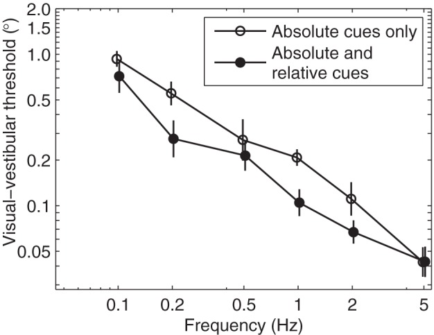
Thresholds are lower when relative visual cues are provided in addition to absolute visual cues. We define relative cues as those in which the motion of space-fixed and body-fixed landmarks can be compared, while absolute cues only provide motion of the visual scene relative to the retina. Open circles are the same condition presented for visual-vestibular (study A) thresholds in which the circular aperture is used to prevent subjects from using relative visual cues. Solid circles are visual-vestibular thresholds for which the aperture was not used, allowing subjects to look for relative cues; for example, one subject reported using their knee as a landmark to judge motion of the visual scene. Averaged across frequencies, thresholds are 30% lower when relative cues are provided. Although the effect of relative visual cues could have been more directly assessed using visual thresholds rather than visual-vestibular thresholds, this was not possible because of the limited space to mount the visual scene on the motion device. While a possible confound is that FOV also increased without the aperture, this is unlikely because visual thresholds are relatively insensitive to FOV, especially above 30° (Fig. 7). Thresholds are geometric means of five subjects, with the bars indicating standard error of the mean.

Optimal multisensory integration in roll tilt with natural cues.

Our study is consistent with other studies demonstrating static optimal integration of visual and vestibular cues (Butler et al. 2010, 2011; De Vrijer et al. 2009; Fetsch et al. 2009, 2012; Gu et al. 2008; Jurgens and Becker 2006). We highlight important similarities and differences below.

First, few studies of optimal integration have been performed using only natural cues. Since at least some studies caution that the way visual cues are presented can disrupt optimal integration (Butler et al. 2011; de Winkel et al. 2010), it was important to utilize a natural visual scene and manipulate thresholds by changing the motion frequency. This contrasts with prior approaches in which one cue is artificially degraded to alter its precision, as in some self-motion perception studies (Butler et al. 2010; Fetsch et al. 2009, 2012; Gu et al. 2008) and other multisensory integration studies (e.g., Ernst and Banks 2002; Landy et al. 1995). In these earlier self-motion studies, the visual cue was artificially manipulated using a 3D computer-generated scene with varying dot movement coherence. In contrast, our approach confirmed optimal static integration, mimicking the earlier findings, but did so without degrading either the visual or vestibular stimuli.

Furthermore, we did not provide conflicting vestibular and visual cues. Cue conflict is common in many self-motion perception studies (Butler et al. 2010; Fetsch et al. 2009, 2012; Jurgens and Becker 2006) and other multisensory integration studies (e.g., Ernst and Banks 2002; Landy et al. 1995). Cue conflict is not necessary to demonstrate optimal integration (e.g., Gu et al. 2008), although it allows the brain's weights for the two cues to be determined.

This study complements a limited number of studies that have investigated visual-vestibular integration in roll tilt. Bayesian integration for static roll orientation has been demonstrated (Clemens et al. 2011; De Vrijer et al. 2009), and perceptual visual-vestibular interaction has been studied in roll tilt (e.g., Dichgans et al. 1972; Zacharias and Young 1981), but this is the first experimental study to examine optimal integration using thresholds determined with dynamic roll tilt stimuli.

Our results are consistent with static linear optimal integration, but other hypotheses could also explain the data. For example, cue integration could occur in a dynamic nonlinear manner. This possibility also exists for related studies (e.g., Butler et al. 2010; Ernst and Banks 2002; Fetsch et al. 2009, 2012; Gu et al. 2008).

Recent work has suggested that individual subjects may use different strategies for integration of self-motion yaw-rotation cues, and that some subjects behave in a manor inconsistent with optimal integration (de Winkel et al. 2013). Most of our individual subject responses seem consistent with optimal integration (Fig. 9), although our measurement variability for each subject was larger than that in the de Winkel et al. study, precluding the use of statistical tests to test individual subject responses.

Fig. 9.

The frequency responses of roll tilt recognition thresholds for individual subjects in studies A and B.

Contribution of other sensory modalities.

When tilted, the component of body weight supported by the side of the chair results in a force that provides tactile cues (Valko et al. 2012). In addition (or alternatively), somatic graviception (e.g., Mittelstaedt 1996) could contribute. Although thresholds measured during motion may include nonvestibular sensory contributions, this would not fundamentally alter any of our conclusions regarding sensory integration, because, even if measured “vestibular” thresholds included significant tactile/somatosensory contributions, visual-vestibular thresholds measured herein would include all of the same vestibular and nonvestibular contributions.

Furthermore, a recent report (Valko et al. 2012) suggests that vestibular cues predominate in the dark. Patients with total bilateral vestibular loss were reported to have higher thresholds in the dark than normal subjects for several different motion directions, including roll tilt. For roll tilt in the dark, the average thresholds for total vestibular loss patients were significantly greater than normal for the frequency range tested herein, which suggests that, for this task in the dark, vestibular cues predominate over all other cues combined. Finally, another recent report suggests that motion direction recognition thresholds are relatively unaffected by device vibration, providing further support for the importance of vestibular cues in motion direction recognition (Chaudhuri et al. 2013).

Reasons for using dynamic roll tilts.

We chose to investigate dynamic roll tilts because this allowed us to study how the brain combines both static (displacement) and dynamic (motion) cues. Such dynamic stimuli are particularly relevant and interesting because both the visual and vestibular systems provide dynamic time-varying motion and displacement signals. Specifically, motion of the visual scene provides both velocity and displacement cues (e.g., Nakayama and Tyler 1981). Similarly, the SCC provide a velocity signal, while the otolith organs provide a tilt (or displacement) signal. Roll tilt thresholds depend on both SCC and otolith cues (Lewis et al. 2011), which was determined by comparing roll tilt thresholds with roll rotation thresholds collected with the subject supine and reliant on SCC cues. Furthermore, preliminary evidence suggests that the brain integrates SCC and otolith cues to determine self-motion more precisely than with either cue individually, as demonstrated by control data collected from one of our subjects in Fig. 10. [This investigation of SCC-otolith integration is described in more detail in a conference abstract (Lim et al. 2009)].

Fig. 10.

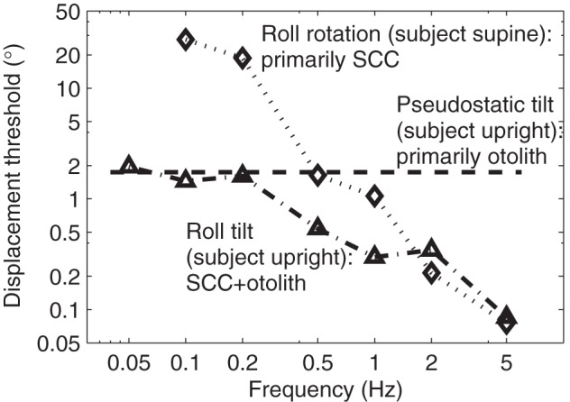
Roll tilt thresholds in the dark likely rely on the integration of semicircular canal (SCC) and otolith organ cues. Roll rotation thresholds (◇) are collected with the subject supine, so that the SCC are the primary motion cue. Pseudostatic-tilt thresholds (dashed line) are collected using very slow constant velocity tilts which stimulate primarily the otolith organ and are consistent with “otolith” thresholds determined by others (Janssen et al. 2011). At low frequencies, roll tilt thresholds are consistent with the pseudostatic-tilt threshold, suggesting the brain relies primarily on otolith organ cues. At high frequencies, roll tilt thresholds are consistent with roll rotation thresholds, suggesting that the brain relies primarily on SCC cues. At intermediate frequencies, roll tilt thresholds are lower than either roll rotation or pseudostatic-tilt thresholds, suggesting that the brain integrates cues to improve precision. (These control data were collected using subject 6 from study A.)

Another advantage of roll-tilt visual motion is that, by definition, it occurs in a plane perpendicular to the line of sight, minimizing potential three-dimensional perspective changes and parallax cues. Furthermore, our design minimizes potential artifacts from the VOR, even if uncompensated centrally (Wade and Curthoys 1997), because torsional VOR gains are ∼0.15 (Bockisch and Haslwanter 2001), much lower than horizontal and vertical VOR gains (Bockisch et al. 2005). While any such artifact would be small, it is also important to note that any such torsional VOR would reduce visual motion on the fovea during the visual-vestibular condition; thus any resulting artifact would make the combined thresholds larger and more suboptimal, rather than leading to a false finding of optimality. It is also unlikely that the oculogyral effect contributes to our results, since it has only been demonstrated for a head-fixed visual target and yaw rotation (e.g., Clark and Stewart 1969), while we used a space-fixed visual scene and roll tilt. While we are unaware of any published studies demonstrating this effect for roll tilt, an abstract has reported that the oculogyral effect did not occur for roll tilt (Kolev and Merfeld 2010).

Rationale for experimental design.

Despite some overlap and differences between studies A and B, each was important to support the primary findings. First, only a single frequency in study A is above the cross-over frequency of 2 Hz, where the data show that vestibular perception can be more precise than visual perception; this necessitated additional data collection above 2 Hz in study B. Second, since optimal integration yields the largest improvement when the individual cues have similar precision (e.g., Ernst and Banks 2002), we chose to do additional testing at frequencies near the cross-over frequency of 2 Hz. While other studies have yielded similar cue precision by degrading visual cues (e.g., Ernst and Banks 2002; Gu et al. 2008), we chose to search for the frequency range where the cues naturally had similar precision. Specifically, if two cues have equal precision, optimal integration yields a combined precision 29% lower than the individual cues' precisions, while, if one cue is three times as precise as the other, optimal integration yields a combined precision that is only 5% lower than the better cue's precision, making statistical evaluation more challenging. Furthermore, statistical testing was aided by making more meticulous thresholds measurements in study B by asking subjects to perform approximately three times as many trials at each frequency. Since most subjects from study A were unavailable or unwilling to participate in further testing, we designed study B as a stand-alone companion study to focus on the range around 2 Hz. Retesting new volunteers at all frequencies would have been a significant burden on volunteers; since total testing time was ∼180 h. Small differences in experimental parameters (e.g., FOV), which were the result of our equipment moving to a different room, had little or no effect. Since we do not directly compare results from studies A and B, any potential subtle differences have no impact on the reported findings.

GRANTS

This research was supported by National Institute of Deafness and Other Communications Disorders Grant R01-DC04158.

DISCLOSURES

No conflicts of interest, financial or otherwise, are declared by the author(s).

AUTHOR CONTRIBUTIONS

Author contributions: F.K. and D.M.M. conception and design of research; F.K. and K.L. performed experiments; F.K. and K.L. analyzed data; F.K., K.L., and D.M.M. interpreted results of experiments; F.K. prepared figures; F.K. drafted manuscript; F.K. and D.M.M. edited and revised manuscript; F.K., K.L., and D.M.M. approved final version of manuscript.

REFERENCES

- Angelaki DE, Yakusheva TA. How vestibular neurons solve the tilt/translation ambiguity. Comparison of brainstem, cerebellum, and thalamus. Ann N Y Acad Sci 1164: 19–28, 2009 [DOI] [PMC free article] [PubMed] [Google Scholar]
- Benson AJ, Hutt EC, Brown SF. Thresholds for the perception of whole body angular movement about a vertical axis. Aviat Space Environ Med 60: 205–213, 1989 [PubMed] [Google Scholar]
- Benson AJ, Spencer MB, Stott JR. Thresholds for the detection of the direction of whole-body, linear movement in the horizontal plane. Aviat Space Environ Med 57: 1088–1096, 1986 [PubMed] [Google Scholar]
- Bles W, Vianney de Jong JM, de Wit G. Compensation for labyrinthine defects examined by use of a tilting room. Acta Otolaryngol (Stockh) 95: 576–579, 1983 [DOI] [PubMed] [Google Scholar]
- Bockisch CJ, Haslwanter T. Three-dimensional eye position during static roll and pitch in humans. Vision Res 41: 2127–2137, 2001 [DOI] [PubMed] [Google Scholar]
- Bockisch CJ, Straumann D, Haslwanter T. Human 3-D aVOR with and without otolith stimulation. Exp Brain Res 161: 358–367, 2005 [DOI] [PubMed] [Google Scholar]
- Butler JS, Campos JL, Bulthoff HH, Smith ST. The role of stereo vision in visual-vestibular integration. Seeing Perceiving 24: 453–470, 2011 [DOI] [PubMed] [Google Scholar]
- Butler JS, Smith ST, Campos JL, Bulthoff HH. Bayesian integration of visual and vestibular signals for heading. J Vis 10: 23, 2010 [DOI] [PubMed] [Google Scholar]
- Chaudhuri SE, Karmali F, Merfeld DM. Whole-body motion-detection tasks can yield much lower thresholds than direction-recognition tasks: implications for the role of vibration. J Neurophysiol 110: 2764–2772, 2013 [DOI] [PMC free article] [PubMed] [Google Scholar]
- Clark B, Stewart JD. Effects of angular acceleration on man: thresholds for the perception of rotation and the oculogyral illusion. Aerospace Med 40: 952–956, 1969 [PubMed] [Google Scholar]
- Clemens IA, De Vrijer M, Selen LP, Van Gisbergen JA, Medendorp WP. Multisensory processing in spatial orientation: an inverse probabilistic approach. J Neurosci 31: 5365–5377, 2011 [DOI] [PMC free article] [PubMed] [Google Scholar]
- Crane BT. Fore-aft translation aftereffects. Exp Brain Res 219: 477–487, 2012a [DOI] [PMC free article] [PubMed] [Google Scholar]
- Crane BT. Roll aftereffects: influence of tilt and inter-stimulus interval. Exp Brain Res 223: 89–98, 2012b [DOI] [PMC free article] [PubMed] [Google Scholar]
- Crawford JD. Living without a balance mechanism. Br J Ophthalmol 48: 357–360, 1964 [DOI] [PMC free article] [PubMed] [Google Scholar]
- Cullen KE. The neural encoding of self-motion. Curr Opin Neurobiol 21: 587–595, 2011 [DOI] [PubMed] [Google Scholar]
- De Vrijer M, Medendorp WP, Van Gisbergen JA. Accuracy-precision trade-off in visual orientation constancy. J Vis 9: 9–15, 2009 [DOI] [PubMed] [Google Scholar]
- de Winkel KN, Soyka F, Barnett-Cowan M, Bulthoff HH, Groen EL, Werkhoven PJ. Integration of visual and inertial cues in the perception of angular self-motion. Exp Brain Res 231: 209–218, 2013 [DOI] [PubMed] [Google Scholar]
- de Winkel KN, Weesie J, Werkhoven PJ, Groen EL. Integration of visual and inertial cues in perceived heading of self-motion. J Vis 10: 1, 2010 [DOI] [PubMed] [Google Scholar]
- Dichgans J, Held R, Young LR, Brandt T. Moving visual scenes influence the apparent direction of gravity. Science 178: 1217–1219, 1972 [DOI] [PubMed] [Google Scholar]
- Dobson A, Barnett A. An Introduction to Generalized Linear Models. Boca Raton, FL: Chapman and Hall/CRC, 2008 [Google Scholar]
- Ernst MO, Banks MS. Humans integrate visual and haptic information in a statistically optimal fashion. Nature 415: 429–433, 2002 [DOI] [PubMed] [Google Scholar]
- Faisal AA, Selen LP, Wolpert DM. Noise in the nervous system. Nat Rev Neurosci 9: 292–303, 2008 [DOI] [PMC free article] [PubMed] [Google Scholar]
- Fetsch CR, DeAngelis GC, Angelaki DE. Visual-vestibular cue integration for heading perception: applications of optimal cue integration theory. Eur J Neurosci 31: 1721–1729, 2010 [DOI] [PMC free article] [PubMed] [Google Scholar]
- Fetsch CR, Pouget A, DeAngelis GC, Angelaki DE. Neural correlates of reliability-based cue weighting during multisensory integration. Nat Neurosci 15: 146–154, 2012 [DOI] [PMC free article] [PubMed] [Google Scholar]
- Fetsch CR, Turner AH, DeAngelis GC, Angelaki DE. Dynamic reweighting of visual and vestibular cues during self-motion perception. J Neurosci 29: 15601–15612, 2009 [DOI] [PMC free article] [PubMed] [Google Scholar]
- Garcia-Perez MA, Alcala-Quintana R. Shifts of the psychometric function: distinguishing bias from perceptual effects. Q J Exp Psychol B 66: 319–337, 2013 [DOI] [PubMed] [Google Scholar]
- Gelb A. Applied Optimal Estimation. Cambridge, MA: MIT, 1992 [Google Scholar]
- Grabherr L, Nicoucar K, Mast FW, Merfeld DM. Vestibular thresholds for yaw rotation about an earth-vertical axis as a function of frequency. Exp Brain Res 186: 677–681, 2008 [DOI] [PubMed] [Google Scholar]
- Green DM, Swets JA. Signal Detection Theory and Psychophysics. New York: Wiley, 1966 [Google Scholar]
- Gu Y, Angelaki DE, DeAngelis GC. Neural correlates of multisensory cue integration in macaque MSTd. Nat Neurosci 11: 1201–1210, 2008 [DOI] [PMC free article] [PubMed] [Google Scholar]
- Haburcakova C, Lewis RF, Merfeld DM. Frequency dependence of vestibuloocular reflex thresholds. J Neurophysiol 107: 973–983, 2012 [DOI] [PMC free article] [PubMed] [Google Scholar]
- Janssen M, Lauvenberg M, van d V, Bloebaum T, Kingma H. Perception threshold for tilt. Otol Neurotol 32: 818–825, 2011 [DOI] [PubMed] [Google Scholar]
- Jurgens R, Becker W. Perception of angular displacement without landmarks: evidence for Bayesian fusion of vestibular, optokinetic, podokinesthetic, and cognitive information. Exp Brain Res 174: 528–543, 2006 [DOI] [PubMed] [Google Scholar]
- Karmali F, Lim K, Adatia A, Claret R, Nicoucar K, Merfeld DM. Perceptual roll tilt thresholds demonstrate visual-vestibular fusion. In: Proceedings of the Eighth Symposium on the Role of the Vestibular Organs in Space Exploration. Washington, DC: NASA Human Research Program, 2011 [Google Scholar]
- Karmali F, Nicoucar K, Lim K, Merfeld DM. Visual-vestibular fusion in sensory recognition thresholds for roll tilt direction. Program No. 677.7/PP1. 2010 Neuroscience Meeting Planner. San Diego, CA: Society for Neuroscience, 2010. [Online] [Google Scholar]
- Kolev O, Merfeld DM. Thresholds for self-motion perception in roll about earth-verical and earth-horizontal axes with and without fixation targets (in Abstracts of the XXVI Barany Society Meeting, Reykjavik, Iceland, August 18–21, 2010). J Vestib Res 20: 287, 2010 [Google Scholar]
- Kolev O, Mergner T, Kimmig H, Becker W. Detection thresholds for object motion and self-motion during vestibular and visuo-oculomotor stimulation. Brain Res Bull 40: 451–457, 1996 [DOI] [PubMed] [Google Scholar]
- Lagace-Nadon S, Allard R, Faubert J. Exploring the spatiotemporal properties of fractal rotation perception. J Vis 9: 3, 2009 [DOI] [PubMed] [Google Scholar]
- Landy MS, Maloney LT, Johnston EB, Young M. Measurement and modeling of depth cue combination: in defense of weak fusion. Vision Res 35: 389–412, 1995 [DOI] [PubMed] [Google Scholar]
- Leek MR. Adaptive procedures in psychophysical research. Percept Psychophys 63: 1279–1292, 2001 [DOI] [PubMed] [Google Scholar]
- Lewis RF, Priesol AJ, Nicoucar K, Lim K, Merfeld DM. Abnormal motion perception in vestibular migraine. Laryngoscope 121: 1124–1125, 2011 [DOI] [PMC free article] [PubMed] [Google Scholar]
- Lim K, Nicoucar K, Merfeld DM. Perceptual direction-detection thresholds for whole body roll tilts about an earth-horizontal axis. Program No. 357.20/AA12. 2009 Neuroscience Meeting Planner. Chicago, IL: Society for Neuroscience, 2009. [Online] [Google Scholar]
- MacNeilage PR, Banks MS, DeAngelis GC, Angelaki DE. Vestibular heading discrimination and sensitivity to linear acceleration in head and world coordinates. J Neurosci 30: 9084–9094, 2010 [DOI] [PMC free article] [PubMed] [Google Scholar]
- Mardirossian V, Karmali F, Merfeld DM. Thresholds for Human Perception of Roll Tilt Motion Depend on Visual-Vestibular Integration. In: Abstracts of the American Neurotology Society Meeting, San Diego, CA. Springfield, IL: American Neurotology Society, 2012 [Google Scholar]
- Merfeld DM. Signal detection theory and vestibular thresholds. I. Basic theory and practical considerations. Exp Brain Res 210: 389–405, 2011 [DOI] [PMC free article] [PubMed] [Google Scholar]
- Merfeld DM, Karmali F, Nicoucar K, Lim K. Perceptual roll tilt thresholds demonstrate visual-vestibular fusion. J Vestib Res 20: 292–293, 2010 [Google Scholar]
- Merfeld DM, Park S, Gianna-Poulin C, Black FO, Wood S. Vestibular perception and action employ qualitatively different mechanisms. I. Frequency response of VOR and perceptual responses during translation and tilt. J Neurophysiol 94: 186–198, 2005a [DOI] [PubMed] [Google Scholar]
- Merfeld DM, Park S, Gianna-Poulin C, Black FO, Wood S. Vestibular perception and action employ qualitatively different mechanisms. II. VOR and perceptual responses during combined tilt and translation. J Neurophysiol 94: 199–205, 2005b [DOI] [PubMed] [Google Scholar]
- Mittelstaedt H. Somatic graviception. Biol Psychol 42: 53–74, 1996 [DOI] [PubMed] [Google Scholar]
- Nakayama K, Tyler CW. Psychophysical isolation of movement sensitivity by removal of familiar position cues. Vision Res 21: 427–433, 1981 [DOI] [PubMed] [Google Scholar]
- Paige GD. Vestibuloocular reflex and its interactions with visual following mechanisms in the squirrel monkey. I. Response characteristics in normal animals. J Neurophysiol 49: 134–151, 1983 [DOI] [PubMed] [Google Scholar]
- Peterka RJ, Benolken MS. Role of somatosensory and vestibular cues in attenuating visually induced human postural sway. Exp Brain Res 105: 101–110, 1995 [DOI] [PubMed] [Google Scholar]
- Robinson DA. Linear addition of optokinetic and vestibular signals in the vestibular nucleus. Exp Brain Res 30: 447–450, 1977 [DOI] [PubMed] [Google Scholar]
- Roditi RE, Crane BT. Directional asymmetries and age effects in human self-motion perception. J Assoc Res Otolaryngol 13: 381–401, 2012a [DOI] [PMC free article] [PubMed] [Google Scholar]
- Roditi RE, Crane BT. Suprathreshold asymmetries in human motion perception. Exp Brain Res 219: 369–379, 2012b [DOI] [PMC free article] [PubMed] [Google Scholar]
- Soyka F, Robuffo GP, Beykirch K, Bulthoff HH. Predicting direction detection thresholds for arbitrary translational acceleration profiles in the horizontal plane. Exp Brain Res 209: 95–107, 2011 [DOI] [PMC free article] [PubMed] [Google Scholar]
- Treutwein B. Adaptive psychophysical procedures. Vision Res 35: 2503–2522, 1995 [PubMed] [Google Scholar]
- Valko Y, Priesol AJ, Lewis RF, Merfeld DM. Contributions of the vestibular labyrinth to human whole-body motion discrimination. J Neurosci 32: 13537–13542, 2012 [DOI] [PMC free article] [PubMed] [Google Scholar]
- Wade SW, Curthoys IS. The effect of ocular torsional position on perception of the roll-tilt of visual stimuli. Vision Res 37: 1071–1078, 1997 [DOI] [PubMed] [Google Scholar]
- Watamaniuk SN, Heinen SJ. Human smooth pursuit direction discrimination. Vision Res 39: 59–70, 1999 [DOI] [PubMed] [Google Scholar]
- Wetherill GB. Sequential estimation of quantal response curves. J R Stat Soc Series B Stat Methodol 25: 1–48, 1963 [Google Scholar]
- Wichmann FA, Hill NJ. The psychometric function. I. Fitting, sampling, and goodness of fit. Percept Psychophys 63: 1293–1313, 2001 [DOI] [PubMed] [Google Scholar]
- Zacharias GL, Young LR. Influence of combined visual and vestibular cues on human perception and control of horizontal rotation. Exp Brain Res 41: 159–171, 1981 [DOI] [PubMed] [Google Scholar]
- Zupan LH, Merfeld DM. Interaural self-motion linear velocity thresholds are shifted by roll vection. Exp Brain Res 191: 505–511, 2008 [DOI] [PMC free article] [PubMed] [Google Scholar]