SIMULATION OF PLANAR SOFT TISSUES USING A STRUCTURAL CONSTITUTIVE MODEL: FINITE ELEMENT IMPLEMENTATION AND VALIDATION

Abstract

Computational implementation of physical and physiologically realistic constitutive models is critical for numerical simulation of soft biological tissues in a variety of biomedical applications. It is well established that the highly nonlinear and anisotropic mechanical behaviors of soft tissues are an emergent behavior of the underlying tissue microstructure. In the present study, we have implemented a structural constitutive model into a finite element framework specialized for membrane tissues. We noted that starting with a single element subjected to uniaxial tension, the non-fibrous tissue matrix must be present to prevent unrealistic tissue deformations. Flexural simulations were used to set the non-fibrous matrix modulus because fibers have little effects on tissue deformation under three-point bending. Multiple deformation modes were simulated, including strip biaxial, planar biaxial with two attachment methods, and membrane inflation. Detailed comparisons with experimental data were undertaken to insure faithful simulations of both the macro-level stress-strain insights into adaptations of the fiber architecture under stress, such as fiber reorientation and fiber recruitment. Results indicated a high degree of fidelity and demonstrated interesting microstructural adaptions to stress and the important role of the underlying tissue matrix. Moreover, we apparently resolve a discrepancy in our 1997 study (J Biomech. 1997 Jul;30(7):753–6) where we observed that under strip biaxial stretch the simulated fiber splay responses were not in good agreement with the experimental results, suggesting non-affine deformations may have occurred. However, by correctly accounting for the isotropic phase of the measured fiber splay, good agreement was obtained. While not the final word, these simulations suggest that affine kinematics for planar collagenous tissues is a reasonable assumption at the macro level. Simulation tools such as these are imperative in the design and simulation of native and engineered tissues.

1. INTRODUCTION

Historically, the term “tissue engineering” is attributed in 1988 to Y.C. Fung (Woo and Seguchi, 1989). The term underscored the importance of “the application of principles and methods of engineering and life sciences toward a fundamental understanding of structure-function relationships in normal and pathologic mammalian tissues and the development of biological substitutes to restore, maintain, or improve tissue function.” Thus, it is imperative that fundamental structure-function understanding guides the reproduction of native tissue if it is to emulate its native counterpart successfully (Butler, Goldstein et al. 2000). A critical step in this process is the development of the constitutive model, which are of fundamental importance for computational simulation and analysis of the mechanical behavior of native and engineered soft biological tissues. For example, surgical simulations and medical device design require reliable constitutive model to accurately predict tissue behavior. Therefore, constitutive modeling of soft biological tissues remains an active, important, and challenging research area.

Traditionally, soft tissues are modeled as pseudo-hyperelastic materials using either phenomenological or structural approaches (Criscione et al., 2003; Holzapfel and Ogden, 2009; Sacks, 2000). A common phenomenological model is the Fung-type (Fung, 1993; Tong and Fung, 1976), in which the strain energy function is a quadratic exponential function of the Green-Lagrange strain tensor. The original form was based on the observed linear relation between tissue stiffness and stress under uniaxial conditions (Fung, 1993). However, phenomenological models lack physical interpretation and cannot, in general, be used for simulations beyond the strain range utilized in parameter estimation. This effect has been shown to be the case even when the strain magnitudes did not exceed the maximum values measured but where substantially far from the available experimental data (Sun et al., 2003). While the underlying reasons for this still need to be elucidated, models which possess greater links to the underlying physical mechanisms appear to be the next step.

Like any biological or synthetic biomaterial, the complex mechanical behavior of soft tissues results from the deformations and interactions of the constituent phases. For most soft tissues, these include collagen, elastin, muscular, and related matrix components such as glycosaminoglycans and proteoglycans. The idea of accounting for tissue structure into mechanical models of soft tissues goes back to at least the work on leather mechanics in 1945 by Mitton (Mitton). More contemporary work on structural approaches followed, with growing popularity in the 1970’s (Beskos and Jenkiins, 1975), with the concept of stochastic constituent fiber recruitment developed about the same time (Soong and Huang, 1973) based on related structural studies (Kenedi et al., 1965). In part a result of the availability of the first planar biaxial data for soft tissues, Lanir developed the first comprehensive, multidimensional structural constitutive model formulation (Lanir, 1979). With various modifications, Lanir et al. applied this approach to many soft tissues such as lung (Lanir, 1983), myocardium (Horowitz et al., 1988).

By linking tissue deformation at macroscopic scale and microscopic (fiber) scale through affine deformation assumption, the structural constitutive model can be considered a statistical multi-scale approach. Above all, structural constitutive modeling approaches can, in principle, provide valuable insight into tissue function. For example, Billiar and Sacks (Billiar and Sacks, 2000a, 2000b) demonstrated for aortic valve leaflets that, using a simplified leaflet structure, angular rotation of the fibers account for such important features such as pronounced mechanical anisotropy, axial coupling, and very large strains (>80%) even though the tissue is composed of collagen fibers that fail at less than ~12 % strain. Later, Sacks demonstrated that with the use of only an equi-biaxial test and the experimentally measured fiber orientation distribution, the complete in-plane biaxial response could be simulated (Sacks, 2003). More recently, structural approaches have been used for a wide range of native and engineered tissue applications, such as elastomeric tissue engineering scaffolds (Courtney et al., 2006), urinary bladder wall (Wognum et al., 2009), and many others (Fata et al., 2014; Hansen et al., 2009; Hollander et al., 2011; Kao et al., 2011).

Due to the need to solve soft tissue problems that involve complex anatomical geometries and boundary conditions, many constitutive models for soft tissues in various forms have been implemented into a computational framework (Driessen et al., 2007; Holzapfel et al., 1996; Prot et al., 2007; Sun and Sacks, 2005) (Hariton et al., 2007). Yet, robust evaluation and rigorous validation of structural constitutive models remain quite limited. Moreover, studies on structural model have mainly focused on either material parameter estimation (Jor et al., 2011) or comparison with different constitutive models (Bischoff, 2006; Cortes et al., 2010; Tonge et al., 2013). Structural models that incorporate fiber recruitment have rarely been used, largely due to computational demands of the additional integration. Recent ability to get detailed fiber recruitment data (e.g. (Chen et al., 2011; Fata et al., 2013; Gleason et al., 2008)) makes this approach all the more relevant. The deep insights that structural models can provide, such as the role of fiber structure and kinematics, still have yet to be fully explored by simulation.

Since many soft tissues are relatively thin, they can be modeled using shell or membrane elements in FE analysis, greatly speeding up the simulations. In the present study, we implemented a planar structural constitutive model into the commercial finite element (FE) package ABAQUS. By numerical simulation of one single element subjected to uniaxial tension, we first revealed that matrix must be present to prevent unrealistic tissue deformations. Flexural simulations were utilized to estimate the matrix modulus, since the underlying collagen fibers remain undulated due to the small extensional strains, and thus have little effect on tissue stress development. Strip biaxial strain and equi-biaxial tension simulations were also performed and compared with experimental collagen fiber measurements to demonstrate the effects of initial fiber orientation distribution on fiber reorientation. Simulation of membrane inflation tests were also applied to further test the structural model. In addition to prediction of macroscopic mechanical response of soft tissues, we demonstrate how the structural model can provide insights into tissue micro-structural events.

2. Methods

2.1 Theoretical formulation

Soft biological tissues primarily have two major load-bearing components: the fibrous network and the non-fibrous (i.e. amorphous) ground matrix. Based on Fung (Fung, 1993), we idealize the elastic behavior of soft tissues as pseudo-hyperelastic composite materials. Thus, the total strain energy function Ψ of soft tissue at a represent volume element (RVE) is defined using

$$\mathrm{\Psi }(\tilde{\mathbf{C}})=\sum _{\mathrm{i}=1}^{\mathrm{n}}{\mathrm{\varphi }}_{\mathrm{f}}^{\mathrm{i}}{\mathrm{\Psi }}_{\mathrm{f}}^{\mathrm{i}}+{\mathrm{\varphi }}_{\mathrm{m}}{\mathrm{\Psi }}_{\mathrm{m}}+\mathrm{p}(\mathrm{J}-1)$$ (1),

where Ψ_f and Ψ_m are the strain energy functions for the fiber and matrix phases, respectively, ${\mathrm{\varphi }}_{\mathrm{f}}^{\mathrm{i}}$ and ϕ_m are the volume fraction of fiber and matrix respectively, with $\sum _{\mathrm{i}=1}^{\mathrm{n}}{\mathrm{\varphi }}_{\mathrm{f}}^{\mathrm{i}}+{\mathrm{\varphi }}_{\mathrm{m}}=1$, J = det (F̃) and p the Lagrange multiplier to enforce incompressibility due to soft tissue’s high water content. The contributions of the non-fibrous components and fluid phases are assumed to be responsible for the incompressibility of the tissue. Based on previous results (Buchanan and Sacks, 2013), we model the matrix phase (which compromises all non-fibrous components) as a single isotropic hyperelastic Neo-Hookean material with the strain energy function Ψ_m = C₁(I_C − 3). Here, I_C is the first invariant of the right Cauchy-Green tensor C̃=F̃^TF̃, and to be consistent with linear elasticity C₁ = μ / 2, where μ is the shear modulus. Using S = ∂Ψ / ∂E, the resulting 2^nd-Piola Kirchhoff stress is given by

$${\mathbf{S}}_{\mathrm{m}}={\mathrm{\varphi }}_{\mathrm{m}}\frac{{\mathrm{C}}_1}{2}({\mathrm{I}}_1-3)-\mathrm{p}{\tilde{\mathbf{C}}}^{-1}$$ (2).

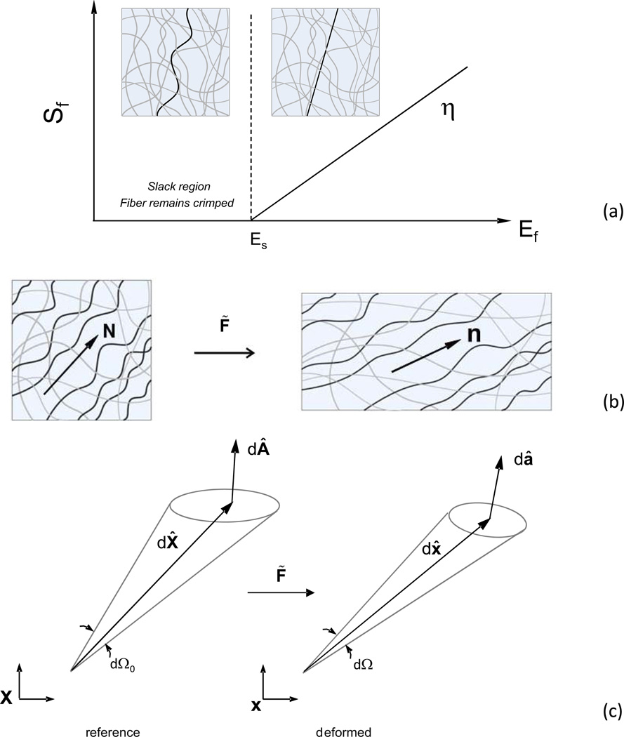
Next, without loss of generality, we focus on a single, undulated Type I collagen fiber type with planar structures and a plane stress state. As in related work on collagenous tissues (Lanir, 1983; Sacks, 2003), we assume a linear S_f = ηE_f relationship for the individual collagen fibers

$${\mathrm{\Psi }}_{\mathrm{f}}({\mathrm{E}}_{\mathrm{f}})=\frac{\mathrm{\eta }}{2}{\mathrm{E}}_{\mathrm{f}}^2$$ (3),

where η is the elastic modulus of individual straight collagen fibers (Fig. 1-a). Due to their crimped structure, we express individual fiber’s true fiber strain using ${\mathrm{E}}_{\mathrm{t}}=\frac{{\mathrm{E}}_{\mathrm{f}}-{\mathrm{E}}_{\mathrm{s}}}{1+2{\mathrm{E}}_{\mathrm{s}}}$ where E_s is the fiber slack strain (Fig. 1-a). The resulting individual collagen fiber strain energy is thus

$${\mathrm{\Psi }}_{\mathrm{f}}({\mathrm{E}}_{\mathrm{t}})=\frac{\mathrm{\eta }}{2}{\mathrm{E}}_{\mathrm{t}}^2=\frac{\mathrm{\eta }}{2}{\left(\frac{{\mathrm{E}}_{\mathrm{f}}-{\mathrm{E}}_{\mathrm{s}}}{1+2{\mathrm{E}}_{\mathrm{s}}}\right)}^2$$ (4).

Figure 1.

(a) Assumed stress-strain response of a single undulated fiber. Graphical depiction of a (b) fiber ensemble and (c) material line, area, and stereo-angle elements before and after deformation.

To develop the first level homogenization, we define a fiber ensemble as the collection of all fibers within the RVE with a common direction N̂ = [cos(θ) sin(θ) 0] (Fig. 1-b). The collective mechanical contribution from the ensemble is represented by its strain energy Ψ_ens. Assuming affine deformation (Lanir, 1983; Sacks, 2003), the fiber ensemble strain E_ens in the direction N̂ is related to the macroscopic tissue-level Green-Lagrange strain tensor $\tilde{\mathbf{E}}=\frac{1}{2}(\tilde{\mathbf{C}}-\tilde{\mathbf{I}})$ by

$${\mathrm{E}}_{\text{ens}}(\mathrm{\theta })={\widehat{\mathbf{N}}}^{\mathbf{T}}\tilde{\mathbf{E}}\widehat{\mathbf{N}}$$ (5).

We make the distinction between fiber and ensemble strains here since individual collagen fibers will have a different strain levels due to their undulations. Note that the non-linearity of the tissue evolves from the gradual recruitment of the linearly elastic collagen fibers (Lanir, 1983), and is thus a structural as opposed to a material property.

To stochastically account for the gradual recruitment of the collagen fiber in each fiber ensemble with strain, we define the function D(E_s) over the ensemble strain range E_ens ∈ [E_lb,E_ub]. Here, E_lb and E_ub represent the lower and upper bounds of collagen fiber ensemble recruitment strain levels, with E_ub > E_lb > 0 and ${\int }_{{\mathrm{E}}_{\text{lb}}}^{{\mathrm{E}}_{\text{ub}}}\mathrm{D}(\mathrm{x})\mathrm{d}\mathrm{x}=1$. The ensuing fiber ensemble strain energy and stress-strain relation are then described as the sum of individual fiber strain energies of the ensemble weighted by the distribution of slack strains D, so that

$${\mathrm{\Psi }}_{\text{ens}}=\frac{\mathrm{\eta }}{2}{\int }_0^{{\mathrm{E}}_{\text{ens}}}\mathrm{D}(\mathrm{x}){\left(\frac{{\mathrm{E}}_{\text{ens}}-\mathrm{x}}{1+2\mathrm{x}}\right)}^2\mathrm{d}\mathrm{x}{\mathrm{S}}_{\text{ens}}=\mathrm{\eta }{\int }_0^{{\mathrm{E}}_{\text{ens}}}\mathrm{D}(\mathrm{x})\frac{{\mathrm{E}}_{\text{ens}}-\mathrm{x}}{{(1+2\mathrm{x})}^2}\mathrm{d}\mathrm{x}$$ (6).

D was represented as a Beta distribution B defined over E_s ∈ [E_lb,E_ub],

$$\mathrm{D}(\mathrm{x})=\{\begin{array}{cc}\frac{{\mathrm{x}}^{\mathrm{\alpha }-1}{(1-\mathrm{x})}^{\mathrm{\beta }-1}}{\mathrm{B}(\mathrm{\alpha },\mathrm{\beta })({\mathrm{E}}_{\text{ub}}-{\mathrm{E}}_{\text{lb}})},\hfill & \text{for}\mathrm{x}\in [0,1]\hfill \\ 0,\hfill & \text{otherwise}\hfill \end{array},\mathrm{x}=({\mathrm{E}}_{\text{ens}}-{\mathrm{E}}_{\text{lb}})/({\mathrm{E}}_{\text{ub}}-{\mathrm{E}}_{\text{lb}})$$ (7),

where α and β are the shape factors. Note that for simplicity we chose E_lb = 0, although generally it is not (Fata et al., 2013).

In situations where computational demands are very high, we also present an alternative formulation for the ensemble stress-strain relation using simplified exponential form that emulates the recruitment behavior at both low and high strains. The novel aspect here is that the terminal stiffness of the fiber ensemble is reproduced for ensemble strains above E_ub. This simple but important modification helps avoid unrealistically high fiber stresses at high strains when using an exponential model alone. For an exponential model, this becomes

$${\mathrm{S}}_{\text{ens}}({\mathrm{E}}_{\text{ens}})=\{\begin{array}{c}\mathrm{A}({\mathrm{e}}^{{\text{BE}}_{\text{ens}}}-1),\text{for}{\mathrm{E}}_{\text{ens}}\le {\mathrm{E}}_{\text{ub}}\\ \mathrm{A}({\mathrm{e}}^{{\text{BE}}_{\text{ub}}}-1)+\text{AB}{\mathrm{e}}^{{\text{BE}}_{\text{ub}}}({\mathrm{E}}_{\text{ens}}-{\mathrm{E}}_{\text{ub}}),\text{for}{\mathrm{E}}_{\text{ens}}>{\mathrm{E}}_{\text{ub}}\end{array}$$ (8),

where A and B are material constants. Note that the tangent modulus is continuous at E = E_ub.

In the final step, we homogenize the ensemble response to the tissue level by defining the tissue strain energy as the sum of the strain energy of fiber ensembles, weighted by the orientation distribution function (ODF) Γ(θ). Thus, we have

$${\mathrm{\Psi }}_{\mathrm{c}}={\int }_{-\mathrm{\pi }/2}^{\mathrm{\pi }/2}\mathrm{\Gamma }(\mathrm{\theta }){\mathrm{\Psi }}_{\text{ens}}({\mathrm{E}}_{\text{ens}})\mathrm{d}\mathrm{\theta }$$ (9),

with the normalization constraint ${\int }_{-\mathrm{\pi }/2}^{\mathrm{\pi }/2}\mathrm{\Gamma }(\mathrm{\theta })\mathrm{d}\mathrm{\theta }$. In summary, the total strain energy function of soft tissue in the RVE is expressed as

$$\mathrm{\Psi }=\frac{{\mathrm{\varphi }}_{\mathrm{f}}\mathrm{\eta }}{2}{\int }_{-\mathrm{\pi }/2}^{\mathrm{\pi }/2}\mathrm{\Gamma }(\mathrm{\theta })[{\int }_0^{{\mathrm{E}}_{\text{ens}}}\mathrm{D}(\mathrm{x}){\left(\frac{{\mathrm{E}}_{\text{ens}}-\mathrm{x}}{1+2\mathrm{x}}\right)}^2\mathrm{d}\mathrm{x}]\mathrm{d}\mathrm{\theta }+\frac{{\mathrm{\varphi }}_{\mathrm{m}}{\mathrm{\mu }}_{\mathrm{m}}}{2}({\mathrm{I}}_1-3)+\mathrm{p}(\mathrm{J}-1)$$ (10).

For the plane stress case, the out of plane stress component S₃₃ = 2 ∂Ψ / ∂C₃₃ = 0, so that the Lagrange multiplier p can be determined directly from

$$\mathrm{p}=-{\mathrm{\varphi }}_{\mathrm{m}}{\mathrm{\mu }}_{\mathrm{m}}{\mathrm{C}}_{33}$$ (11).

The total second Piola-Kirchhoff stress can be thus written as

$$\tilde{\mathbf{S}}={\mathrm{\varphi }}_{\mathrm{f}}{\mathrm{\eta }}_{\mathrm{f}}{\int }_{-\mathrm{\pi }/2}^{\mathrm{\pi }/2}\mathrm{\Gamma }(\mathrm{\theta })[{\int }_0^{{\mathrm{E}}_{\text{ens}}}\mathrm{D}(\mathrm{x})\frac{{\mathrm{E}}_{\text{ens}}-\mathrm{x}}{{(1+2\mathrm{x})}^2}\mathrm{d}\mathrm{x}](\widehat{\mathbf{N}}\otimes \widehat{\mathbf{N}})\mathrm{d}\mathrm{\theta }+{\mathrm{\varphi }}_{\mathrm{m}}{\mathrm{\mu }}_{\mathrm{m}}(\tilde{\mathbf{I}}-{\mathrm{C}}_{33}{\tilde{\mathbf{C}}}^{-1})$$ (12).

for the recruitment model, and

$$\tilde{\mathbf{S}}={\int }_{-\mathrm{\pi }/2}^{\mathrm{\pi }/2}\mathrm{\Gamma }(\mathrm{\theta }){\mathrm{S}}_{\text{ens}}[{\mathrm{E}}_{\text{ens}}(\mathrm{\theta })](\widehat{\mathbf{N}}\otimes \widehat{\mathbf{N}})\mathrm{d}\mathrm{\theta }+{\mathrm{\varphi }}_{\mathrm{m}}{\mathrm{\mu }}_{\mathrm{m}}(\tilde{\mathbf{I}}-{\mathbf{C}}_{33}{\tilde{\mathrm{C}}}^{-1})$$ (13).

for the simplified model (Eqn. 8).

2.2 Finite element implementation

The structural model was implemented into commercial finite element software ABAQUS/Standard (Dassault Systemes Simulia Corp., Providence, RI) via user defined material subroutine UMAT. The stress tensor components utilized in UMAT is defined in a co-rotational coordinate system in which the local material axes defined in the initial configuration rotates with the material (ABAQUS, 2011). Using polar decomposition theorem (Marsden and Hughes, 1983) we have F̃ = R̃Ũ, where R̃ is the rigid body rotation tensor and Ũ is the right symmetric stretch tensor. Also, the rotated Cauchy stress can be determined using t̃ = J⁻¹ŨS̃Ũ and the fourth-rank material elasticity tensor ℂ^SE are updated in the UMAT code (see appendix for details).

In the actual implementation, S̃ and ℂ^SE require integration over θ ∈ [−π / 2, π/ 2] as well as E_ens ∈ [E_lb,E_ub]. Since a closed form solutions are not available in general, a numerical integration scheme was used as follows. During implementation, the angle domain and the fiber strain domain were separated into twenty segments with equal size. In each segment, Gaussian quadrature integration rule (Hughes, 2000) was performed with five integration points.

2.2 Further model modifications and material parameter estimation

For the present work we merged (without loss of generality) the material parameters ϕ_m and μ_m for matrix component into μ_m, as well as ϕ_f and η for the fiber component were also combined into η. Due to its high collagen Type I content, generally planar tissue architecture, well characterized structure and mechanical properties, and previous use in structural models (Sacks, 2003) made native bovine pericardium natural choice for the representative tissue for simulations. To obtain the value for μ_m, we utilized flexural data from native bovine pericardium (Mirnajafi et al., 2005). In that study, a nearly linear moment-curvature relation has been observed. This suggested that the collagen fibers have little effect in flexure, which is consistent with the very low strains that occur in this deformation mode (so that the collagen fibers remain fully undulated and only the matrix contributes). We thus obtained μ_m by fitting the moment-curvature curve (Mirnajafi et al., 2005), using methods described in the next section.

The total fiber angular distribution function is expressed as a linear combination of Gaussian distribution and uniform distribution

$$\mathrm{\Gamma }(\mathrm{\theta })=\mathrm{d}\left[\frac{\text{exp}(-\frac{{\mathrm{\theta }}^2}{2{\mathrm{\sigma }}^2})}{\text{erf}(\frac{\mathrm{\pi }}{2\sqrt{2}\mathrm{\sigma }})\sqrt{2\mathrm{\pi }}\mathrm{\sigma }}\right]+\frac{(1-\mathrm{d})}{\mathrm{\pi }}$$ (14).

Eqn. (14) was chosen to allow graduations in aligned and isotropic fiber distributions to be simulated easily. Here σ denotes the standard deviation of the Gaussian distribution function, and the error function erf() is introduced so that the integration of the Gaussian distribution function over angle domain θ ∈[−π / 2,π/ 2] is equal to unity. The fiber angular distribution function was obtained previous measurements and fitting the experimental data with d=1 (Billiar and Sacks, 1997).

One way to evaluate the robustness and accuracy of the FE implementation is to examine applications where very large strains are known to occur, which induce large fiber rotations and stretches. Previous experimental results have revealed that the mechanical behavior of soft collagenous tissue are strongly dependent on gripping methods (Waldman and Lee, 2002). In particular, we noted in that study that clamps induced large rotations in the corner regions between the clamps. Thus, the material parameters from both model forms were obtained by fitting stress-strain curve from the equi-biaxial loading stress-strain data with suturing arrangement from (Waldman and Lee, 2002). This allowed us to directly compare the FE results to the experimental findings from that study.

2.4 Finite element simulations

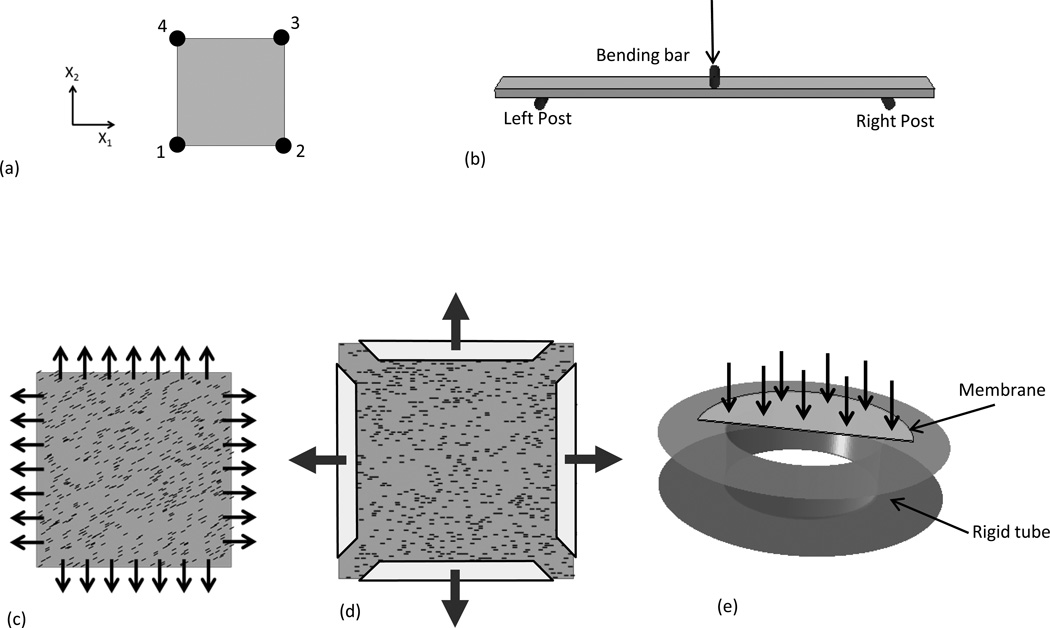
We start with a basic simulation of a single element under uniaxial tension to investigate the effects of matrix. For this example, a square element was subjected to uniaxial strain in X₁ direction (Fig. 2-a). Nodes 1 and 2 were constrained in X₂ direction, and nodes 1 and 4 were constrained in the X₁ direction, with uniform displacements applied to nodes 2 and 3 in X₁ direction. The preferred fiber orientation coincided with the X₁ direction. Next, to verify minimal fiber recruitment occurred during flexure, simulation of a bending test was performed. The length and width of the specimen used for bending simulation is 20.0 mm and 3.0 mm respectively, with the thickness of the tissue is 0.4 mm and the span 16.0 mm (Fig. 2-b). The loading was applied at the center of the tissue through the middle post, with the three posts were considered as rigid bodies. The friction coefficient was assumed to be zero for the tissue in contact with the left and right posts. All the material parameters for native bovine pericardium are summarized in Table 1.

Figure 2.

Schematic overview of the simulation setup. (a) One four node element, (b) three-point bending configuration, (c) strip biaxial tension with seven sutures along each side and initial fiber orientation, (d) equi-biaxial tension with clamped boundary condition and initial fiber orientation, (e) inflation of fetal membrane, with only half of the membrane was modeled due to symmetry.

Table 1.

Material Parameters for native bovine pericardium (BP) and the fetal membrane (FM)

Material	ϕfη(kPa)	σ	α	β	εub	ϕmμ (kPa)	ϕfA (kPa)	B
BP	20996.7	38°	6.43	1.01	0.25	100.0	0.157	31.256
FM	40480.0	-	10.74	1.06	0.75	21.0	-	-

To investigate the effects of both boundary conditions (as both localized point and distributed loads) on fiber reorientation, we simulated native bovine pericardium using sutures under strip biaxial tension using data from (Billiar and Sacks, 1997) and equi-biaxial tension using clamped boundary conditions using data from (Waldman et al., 2002). To simulate both high and low orientations, we utilized two levels of d (d=1.0 and d=0.25). For the first test, the dimensions of the specimen were 19.2 mm X 19.2 mm and the thickness is 0.4 mm. As in the original experiment, uniform displacements were applied on the seven suture attachment points along each side the specimen, with the initial preferred fiber orientation set to 27° from the X₁ axis (Fig. 2-c). Two loading cases were considered; 30% along X₁ direction/0% for the X₂, and 30% along the X₂ direction/0% along the X₁. For the clamped equi-biaxial tension test, the dimensions of the specimen were 22.0 mm X 22.0 mm (Fig. 2-d) and the thickness 0.4 mm. The tissue was stretched 10% in X₁ and X₂ directions. The initial fiber orientation was assumed to be the X₁ direction (Fig. 2-d).

As a final test, we simulated a fetal membrane (FM) inflation test using data from Joyce et al. (Joyce et al., 2009). Uniform pressure was applied on the top surface of a circular membrane and only half of the tissue was modeled due to symmetry (Fig. 2-e). The radius of the circular membrane was 21.0 mm and the thickness 0.228 mm. The tube was modeled as rigid body with an inner radius of 15.0 mm and the edge of the tissue fixed. SALS measurements of the intact FM (Joyce et al., 2009) revealed that the tissue contains no preferred collagen direction, therefore a uniform fiber angular distribution function Γ(θ) = 1 / π was utilized. The friction coefficient was assumed to be zero for the contact interaction of tissue with the rigid tube. Note that for flexural simulations, four-node quadrilateral shell elements were used, and for all the other simulations four-node quadrilateral membrane elements were used.

2.5 Simulation post processing

To provide insights into the deformations of soft tissue microstructure under strain, we implemented the following post-processing procedures. We start by describing generalized methods for transforming the ODF (eqn. 14) under a generalized affine deformation, following methods developed for plasticity (Dafalias, 2001). Within an infinitesimal region of tissue we consider a fiber direction in the undeformed configuration by the vector dX̂ (Fig. 1-c). Under deformation this vector is transformed into the current configuration to dx̂ by dx̂ = F̃ dX̂, with associated stretch $\mathrm{\lambda }=\mathrm{d}\widehat{\mathbf{x}}/\mathrm{d}\widehat{\mathbf{X}}=\sqrt{\widehat{\mathbf{N}}·\tilde{\mathbf{C}}·\widehat{\mathbf{N}}}$. A stereo-angle element dΩ₀ can be defined with respect to dX̂ in the reference configuration, which is transformed in the deformed state to dΩ. The projection of the area vector d onto dX̂ divided by the magnitude of dX̂ can be used to define the angle element dΩ₀, defined by the inner product d÷dX̃ / |dX̃|. This leads to expressions for the angle elements in the reference and current configurations

$$\mathrm{d}{\mathrm{\Omega }}_0=\frac{\mathrm{d}\tilde{\mathbf{A}}·\mathrm{d}\widehat{\mathbf{X}}}{|\mathrm{d}\widehat{\mathbf{X}}{|}^3}\mathrm{d}\mathrm{\Omega }=\frac{\mathrm{d}\widehat{\mathbf{a}}·\mathrm{d}\widehat{\mathbf{x}}}{|\mathrm{d}\widehat{\mathbf{x}}{|}^3}$$ (15).

A fundamental property of affine fiber kinematics states that the total number of fibers, N_f, contained within an angular increment must be preserved under deformation. Relating this condition to ODFs gives

$${\mathrm{N}}_{\mathrm{f}}\mathrm{\Gamma }({\mathrm{\Omega }}_0)\mathrm{d}{\mathrm{\Omega }}_0={\mathrm{N}}_{\mathrm{f}}{\mathrm{\Gamma }}_{\mathrm{t}}(\mathrm{\Omega })\mathrm{d}\mathrm{\Omega }$$ (16),

where Γ_t(Ω) is the fiber orientation deformation function in the deformed stated. This leads immediately to

$$\frac{{\mathrm{\Gamma }}_{\mathrm{t}}(\mathrm{\Omega })}{\mathrm{\Gamma }({\mathrm{\Omega }}_0)}=\frac{\mathrm{d}{\mathrm{\Omega }}_0}{\mathrm{d}\mathrm{\Omega }}$$ (17)

According to Nanson’s relation dâ = JF̃^−Td (Fung, 1965), hence dâ · dx̂ = JF̃^−Td · F̃dX̂ = Jd · dX̂, and with Eqn. 17, yields

$${\mathrm{\Gamma }}_{\mathrm{t}}(\mathrm{\Omega })=\mathrm{\Gamma }({\mathrm{\Omega }}_0)\frac{{\mathrm{\lambda }}^3}{\mathrm{J}}$$ (18).

Eqn. 18 provides a means to determine the ODF in the deformed state in terms of the reference ODF and F̃. Further, the three-dimensional relationship can be reduced to the following two-dimensional form

$${\mathrm{\Gamma }}_{\mathrm{t}}(\mathrm{\beta })=\mathrm{\Gamma }(\mathrm{\theta })\frac{{\mathrm{\lambda }}^2}{{\mathrm{J}}_{2\mathrm{D}}}=\mathrm{\Gamma }(\mathrm{\theta })\frac{\widehat{\mathbf{N}}·\tilde{\mathbf{C}}·\widehat{\mathbf{N}}}{\det \left[{\tilde{\mathbf{F}}}_{2\mathrm{D}}\right]}$$ (19),

where J_2D is the determinate of the in-plane deformation gradient. Note that Γ_t(β) should be plotted against the deformed fiber angle $\mathrm{\beta }={\text{tan}}^{-1}\left(\frac{{\mathrm{F}}_{21}\text{cos}(\mathrm{\theta })+{\mathrm{F}}_{22}\text{sin}(\mathrm{\theta })}{{\mathrm{F}}_{11}\text{cos}(\mathrm{\theta })+{\mathrm{F}}_{12}\text{sin}(\mathrm{\theta })}\right)$ since it refers to the deformed (convected) fiber direction.

In addition to its ability to provide high fidelity simulations of the stress-strain behaviors, the structural model also provides a great deal of information structural adaptation to within the RVE. These are usually overlooked in the literature. Thus, in the present study we defined the fractional ensemble fiber recruitment (FEFR) structural metric for a given direction as

$$\text{FEFR}(\mathrm{\theta })={\int }_0^{{\mathrm{E}}_{\text{ens}}(\mathrm{\theta })}\mathrm{D}(\mathrm{x})\mathrm{d}\mathrm{x}$$ (20).

In addition, the total fiber recruitment (TFR) structural metric for a given RVE was defined as

$$\text{TFR}={\int }_{-\mathrm{\pi }/2}^{\mathrm{\pi }/2}\mathrm{\Gamma }(\mathrm{\theta })[{\int }_0^{{\mathrm{E}}_{\text{ens}}(\mathrm{\theta })}\mathrm{D}(\mathrm{x})\mathrm{d}\mathrm{x}]\mathrm{d}\mathrm{\theta }$$ (21).

Note that both metrics are expressed using a percentile scale.

3. RESULTS

3.1 Uniaxial tension simulation

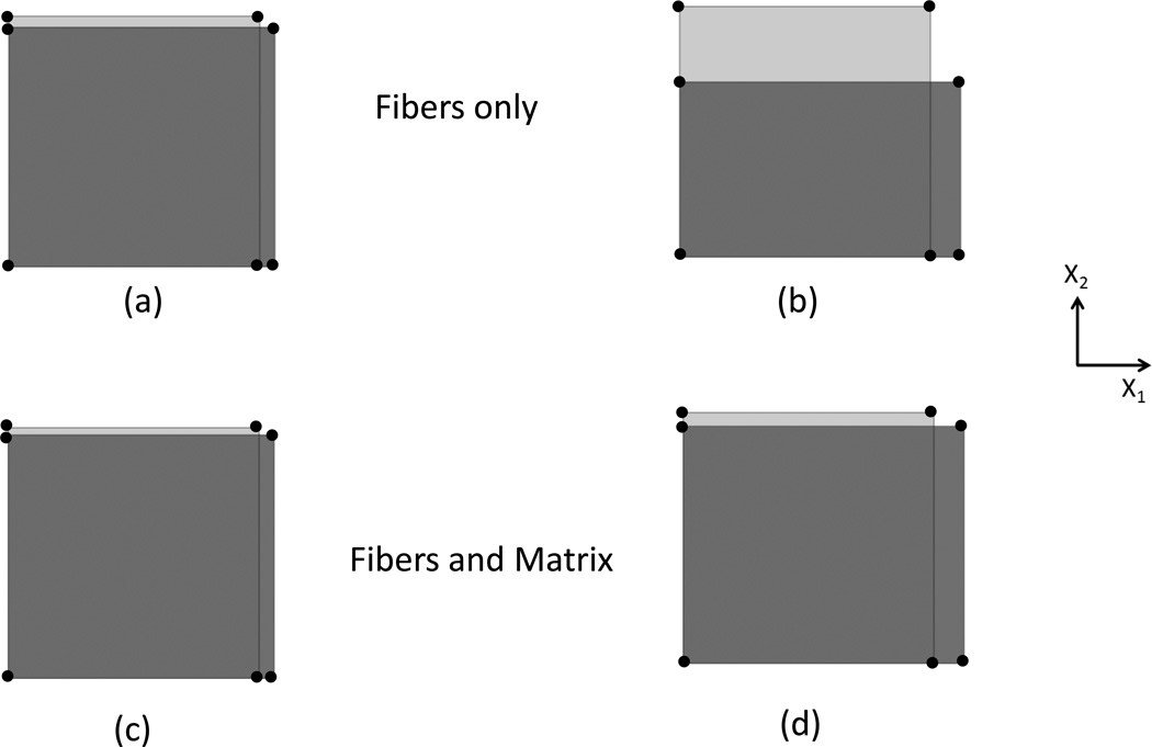
Overall, we determined that the matrix had a signification effect on the simulated deformation of soft tissue under uniaxial tension (Fig. 3). When the tissue is modeled with fibers only, the lateral deformation of the tissue may be unrealistic. Specifically, since under uniaxial tension the stress component in the X₂ direction is ${\mathrm{S}}_{22}={\int }_{-\mathrm{\pi }/2}^{\mathrm{\pi }/2}\mathrm{\Gamma }(\mathrm{\theta }){\mathrm{S}}_{\text{ens}}({\mathrm{E}}_{\text{ens}}){\text{sin}}^2(\mathrm{\theta })\mathrm{d}\mathrm{\theta }$, with S_ens = D(x) = 0 in this direction since the fibers cannot carry any load when compressed. Since Γ (θ) ≥ 0 and sin² (θ) ≥ 0, S₂₂ must be greater than zero, yet under uniaxial tension S₂₂=0, so that an equilibrium state cannot be achieved. For example, when the element is stretched 6% (Fig. 3-a) the Green-Lagrange strain E₁₁=0.618 and E₂₂=−0.0434 with a ratio of −E₂₂/E₁₁ of 0.702. When the element is stretched 12% (Fig. 3-b), the strain ratio −E₂₂/E₁₁ increased to 2.049. The deformation in X₂ direction is larger than that in X₁ direction, and the element collapses to a single line when the stretch ratio is greater than 15%. However, when the matrix is included, the strain ratio −E₂₂/E₁₁ is 0.459 and 0.424 as the element is stretched 6% (Fig. 3-c) and 12% (Fig. 3-d) respectively, so that the deformation of the element is acceptable. Thus for the present model a matrix should be present and in sufficient quantity in the structural model to prevent unphysical characterization of the mechanical behavior of soft tissues under uniaxial tension.

Figure 3.

Undeformed and deformed configuration of one single element under uniaxial tension, under the following conditions: With fibers only stretched 6% (a) and 12% (b), and with fibers and matrix 6% (c) and 12% (d).

3.2 Flexural simulations

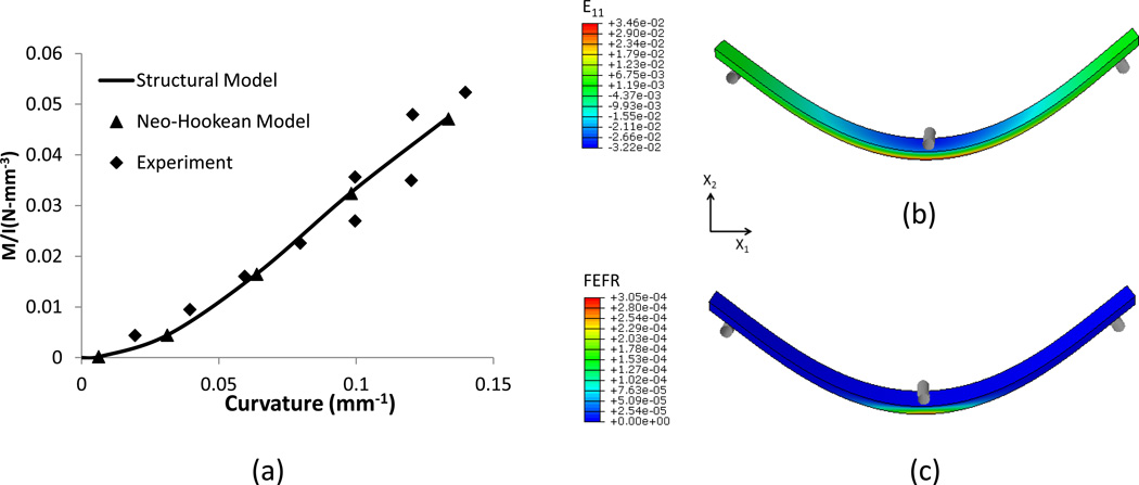
The moment-curvature curves from FE simulation using only the isotropic neo-Hookean model were in good agreement with the published experimental results (Mirnajafi et al., 2005) (Fig. 4-a). The simulation results also confirmed that collagen fiber contributions were negligible; the moment-curvature curves from FE simulations are the same using Neo-Hookean model and the structural model with both fiber and matrix (Fig. 4). The maximum tensile strain (Green-Lagrange strain) under bending was 0.0346 located at the bottom surface. Virtually all (>99%) of the fibers were still undulated in this loading configuration (Fig.4-c); supporting our use of these studies to determine ground matrix mechanical behavior.

Figure 4.

Effective deformations of fibers on soft tissues under three-point bending showing (a) the moment-curvature curve relation obtained using a Neo-Hookean model with matrix only and structural model with fiber and matrix, (b) Green Strain E₁₁ contour, (c) Fractional ensemble fiber recruitment contour in X₁ direction.

3.3 Biaxial test simulations – sutured boundary conditions

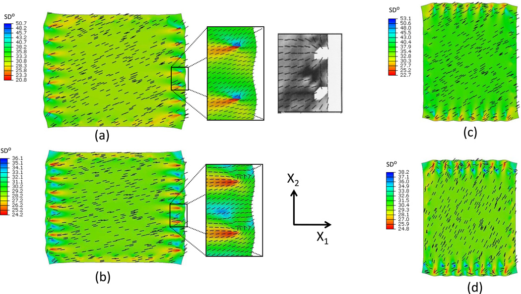
For the strip biaxial test stretched in the X₁ direction, fiber orientation from SALS measurements (Billiar and Sacks, 1997) revealed that the overall preferred fiber direction was reoriented towards the direction of stretch and the degree of fiber alignment was increased. When d=1.0 in the fiber angular density function, the preferred fiber direction rotated only about 4° toward the stretch direction (Fig. 5-a). However, for d=0.25, the preferred fiber direction rotated about 15° toward the stretch direction (Fig. 5-b), in agreement with SALS measurements (Billiar and Sacks, 1997). Around the suture points, the simulation results with d=0.25 (Fig. 5-b) demonstrated that the preferred fiber direction rotated towards the suture points, also in agreement with the SALS data (Billiar and Sacks, 1997). When the tissue was stretched in the X₂ direction with d=1.0, the overall preferred fiber direction reoriented only about 4° towards the stretch direction (Fig. 5-c). While for d=0.25, the overall preferred fiber direction reoriented about 35.0° towards the stretch direction (Fig. 5-d).

Figure 5.

Preferred fiber reorientation and standard deviation contour of fiber angular distribution function from simulation under strip biaxial stretch (a) in X₁ direction with d=1.0, (b) in X₁ direction with d=0.25, (c) in X₂ direction with d=1.0, (d) in X₂ direction with d=0.25. Inset – measured SALS data from the Billiar and Sacks 1997 study, showing very good agreement.

When the tissue was stretched in the X₁ (preferred) direction, more fibers are recruited in the X₁ direction than those in the X₂ direction. For d=0.25, the polar FEFR plot (Fig. 6-a) under different stretch ratios revealed the increasing FEFR in all directions. At λ = 1.18 the FEFR in all directions was less than 20%. As the stretch increased to 1.21, more than 40% of fibers were recruited in the X₁ direction. All the fibers in the X₁ direction were straighten when the strain in X₁ direction just reaches the upper bound strain at λ = 1.24, with all fibers within 24° from the X₁ direction straightened by a stretch of 1.4. The total fiber recruitment (TFR) is 40% uniformly distributed in the center region of the soft tissue (Fig. 6-b and Fig. 6-c). The maximum TFR occurs at the suture points (Fig. 6-b and Fig. 6-c) due to stress concentration.

Figure 6.

(a) Azimuthal plot of the fractional ensemble fiber recruitment under different stretch ratios, (b) Total percentage of fiber recruitment contour after stretch in X₁ direction, (c) Total percentage of fiber recruitment along the line X₁ and X₂ in (b).

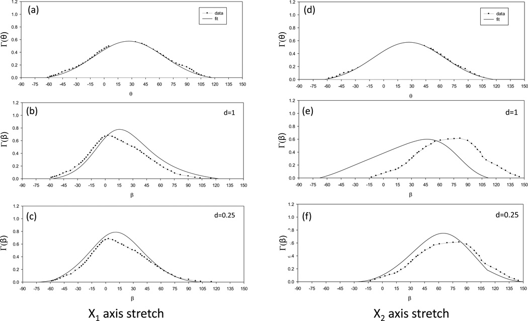
To obtain further insight as to why variations in d lead to different fiber reorganization patterns, we examined the angular distribution of fiber density at the center of the tissue before and after deformation with SALS data taken for bovine pericardium from the 1997 study (Billiar and Sacks, 1997) (Fig. 7). The angular distribution after deformation was computed using the deformation at the tissue center from simulation. Moreover, the fiber angular distribution was renormalized with the baseline removed for values of d of 1.0 and 0.25. As noted in the 1997 study, when the tissue was stretched in the X₁ direction with F=diag[1.3, 1.0], the experimentally determined mean preferred fiber direction shifted from ~30° (Fig. 7-a) to ~15° (Fig. 7-b). While both values of d simulated this shift well, a value of d=0.25 produced a better fit (Figs. 7-b,c). In contrast, when the tissue was stretched in the X₂ direction with F=diag[1.0, 1.3], the experimentally determined mean preferred fiber direction shifted from ~30° (Fig. 7-b) to ~75° (Fig. 7-e). For both deformation states, better agreement was obtained when d=0.25, especially when the tissue was stretched in the X₂ direction (Figs. 7-c,e).

Figure 7.

Fiber angular distribution before and after stretch from SALS data from the Billiar and Sacks 1997 paper and simulation results with d=1.0 and d=0.25. To emulate the original data processing, both the original and simulated distributions were renormalized with the baseline component of the distribution removed.

3.4 Biaxial test simulations – clamped boundary conditions

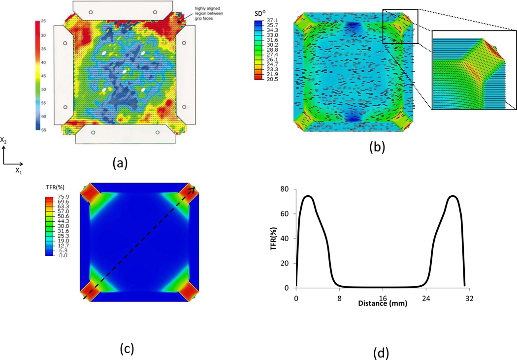
For the tissue with clamped boundary conditions, SALS measurements (Waldman et al., 2002) indicated that fibers between grip faces were highly aligned due to shearing (Fig. 8-a). The preferred fiber orientation rotated about 37.0° at the corner regions from simulation with d=0.25. The distribution of the standard deviation of fiber density from simulation is similar to the distribution of orientation index (OI) from SALS measurements. The structural model provided deep insights into the deformation of fibers. All the fibers initially undulated were straightened gradually with increasing load. Less than 1% of fibers were recruited in the center region of the tissue specimen and more than 70% of fibers in the corner regions were recruited. Along the diagonal line, the TFR is uniformly distributed around the center region of the tissue specimen. The TFR increased dramatically at the corner regions due to large shear strain.

Figure 8.

(a) SALS data (Waldman et al., 2002); (b) Preferred fiber orientation and standard deviation contour of fiber angular distribution function from simulation with d=0.25, (c) Total percentage of fiber recruitment contour, (d) Total percentage of fiber recruitment along the diagonal line in (c).

3.5 Membrane Inflation simulations

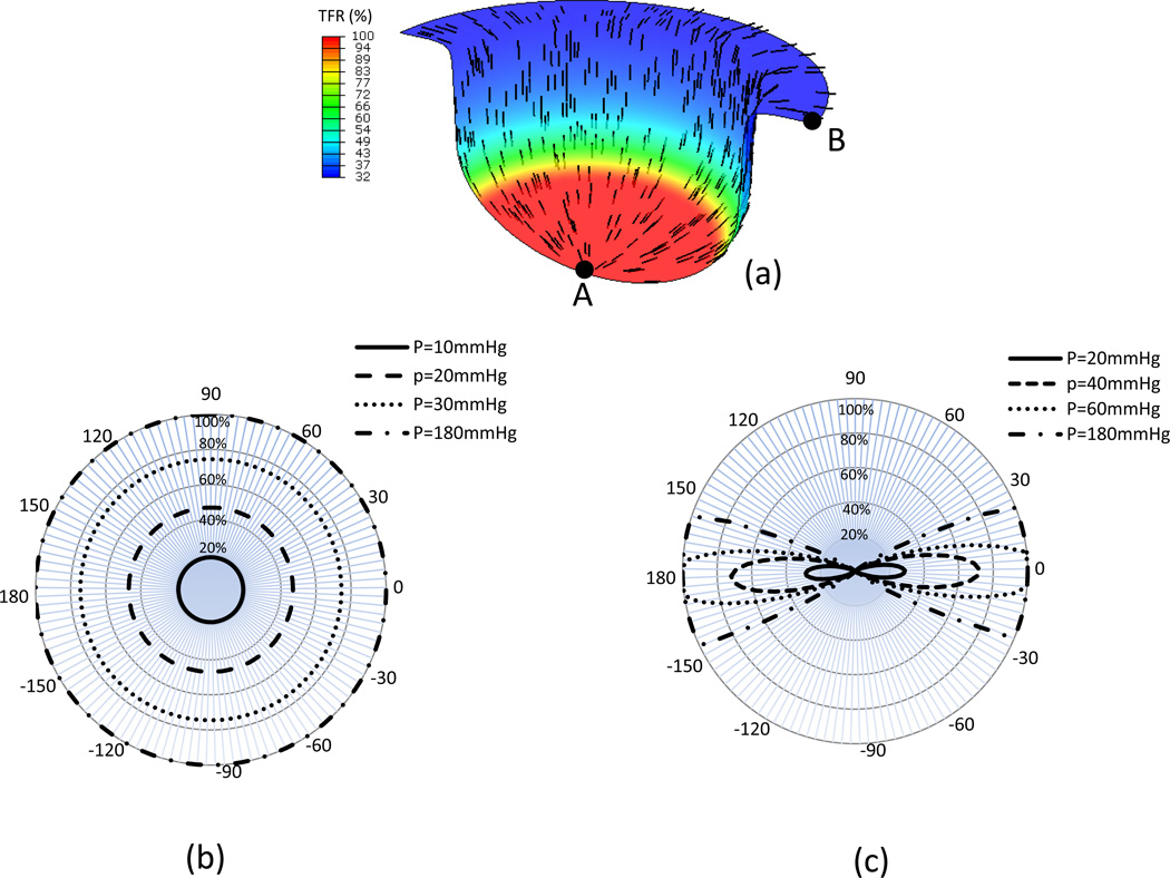
Simulation results revealed that all fibers around the center dome region were straightened (Fig. 9-a). The preferred fiber direction in the deformed shape was rotated to the radial direction of the tissue (Fig. 9-a). The total fiber recruitment decreased gradually from 100% in the center region to 32% at the edge (Fig. 9-a). For element A (Fig. 9-a) at the center of tissue, the strain is the same in each direction. Therefore the fractional ensemble fiber recruitment is equal in each direction (Fig. 9-b). However for location B (Fig. 9-a) at the tissue edge, the strain in the radial direction is larger than that in the circumferential direction. More fibers were recruited in the radial direction (Fig. 9-c).

Figure 9.

Results from the membrane inflation simulations showing (a) preferred fiber orientation and total percentage of fiber recruitment contour from simulation, and the azimuthal plot of the fractional ensemble fiber recruitment of the elements located at (b) element A and (c) element B. Note here that while increased pressure loading predictably increased the total amount of fiber recruitment at both locations, substantial angular variations with pressure was observed at element B.

4 DISCUSSION

4.1 Overall findings

A framework for the implementation of a structural constitutive model for soft tissues into a finite element framework was developed and validated. Simulation of a single element under uniaxial tension revealed that when using fiber systems with angular dispersion, a matrix phase must be present to prevent non-physiological deformations (Fig. 3). This finding may shed insight into how the non-collagenous components of soft tissues play an important role guiding the overall mechanical responses. For example, Lake and Barocas (Lake and Barocas, 2011) studied the effects of simulated non-fibrillar matrix using an agarose analog on the behavior of a collagen-agarose co-gel in uniaxial tension. They reported that the Poisson’s ratio of co-gel decreased from a range of 1.5–3.0 (with a large volume decrease) with no agarose to ~0.5 (i.e. nearly incompressible) with high concentration of agarose. Thus, both the experimental results and the present simulation results suggest that matrix phase may have significant effects on the mechanical behavior of soft tissues.

Biaxial tension simulations demonstrated that the presence of an isotropically oriented fiber phase can significantly affect the overall fiber orientation in the deformed configuration (Fig. 5). For d=1.0, the preferred fiber orientations were far from the SALS measurement for both strip biaxial tests and equi-biaxial tests (Fig. 7). However, simulation results with d=0.25 are in good agreement with the SALS measurement. Not surprisingly, this observation revealed that accurate measurement of the fiber ODF is critical to the structural model.

Invariant based (Spencer, 1972) constitutive models have also been developed for the arterial wall (Gasser et al., 2006) and the aortic valve (Freed et al., 2005). The advantage of these invariant based models is being computationally more efficient. Other have utilized generalized structure tensors in attempt to eliminate the need for numerical integration (Cortes et al., 2010; Federico and Gasser, 2010). However, in this approach the fiber strains are averaged over all orientations, and has lead to less effective fits to the data (Cortes et al., 2010). A closed-form solution using a von Mises distribution function and an exponential fiber stress-strain law has been also been utilized (Raghupathy and Barocas, 2009). However, the closed form is only available for some special statistical functions and not for the recruitment model.

4.2 Convexity of the strain energy function

Strain energy functions for hyperplastic materials must satisfy certain conditions to prevent unphysical material behavior characterization (Truesdell and Noll, 1965). The strong ellipticity condition (Marsden and Hughes, 1983; Truesdell and Noll, 1965) requires that elasticity tensor be positive definite. Moreover the material Jacobian matrix required for finite element simulation must be positive definite to avoid numerical instability. Holzapfel et al. (Holzapfel and Gasser, 2000) discussed the convexity of strain energy functions for several phenomenal models. Sun et al. (Sun and Sacks, 2005) proposed a necessary condition for fitting Fung-type strain energy functions about zero strain. The constraints condition enforced on material parameters guarantees that the second elasticity tensor is positive definite in the reference configuration. Federico et al. (Federico et al., 2008) proved that the necessary condition is also a sufficient condition for the convexity of Fung-type stain energy functions. The convexity of strain energy functions for invariant based structural model was proved by Holzapfel et al. (Gasser et al., 2006; Holzapfel et al., 2004). Lanir (Lanir, 1994, 1996) proved that the Coleman and Noll condition (Truesdell and Noll, 1965) and the strong ellipticity condition are satisfied for the structural model since the fiber’s stretch force increases monotonically with stretch.

4.3 New structural insights

Unlike phenomenological models, the structural model provides more than just stress-strain relationship at the tissue scale. By incorporating fiber orientation distribution and fiber recruitment distribution at tissue microscopic scale, the model can provide information on how soft tissues internally reorganize to external loads by adjusting their internal microstructure. The information include change of fiber angular density, change of preferred fiber orientation, change of fiber recruitment in any orientation, and change of the overall fiber recruitment. The new indices introduced herein provide both single ensemble and total tissue insights into how undulated fiber adapt to the local strain environment. These metrics are particularly useful in understanding structural adaptations and could be directly used in structural optimization studies in engineered tissue design.

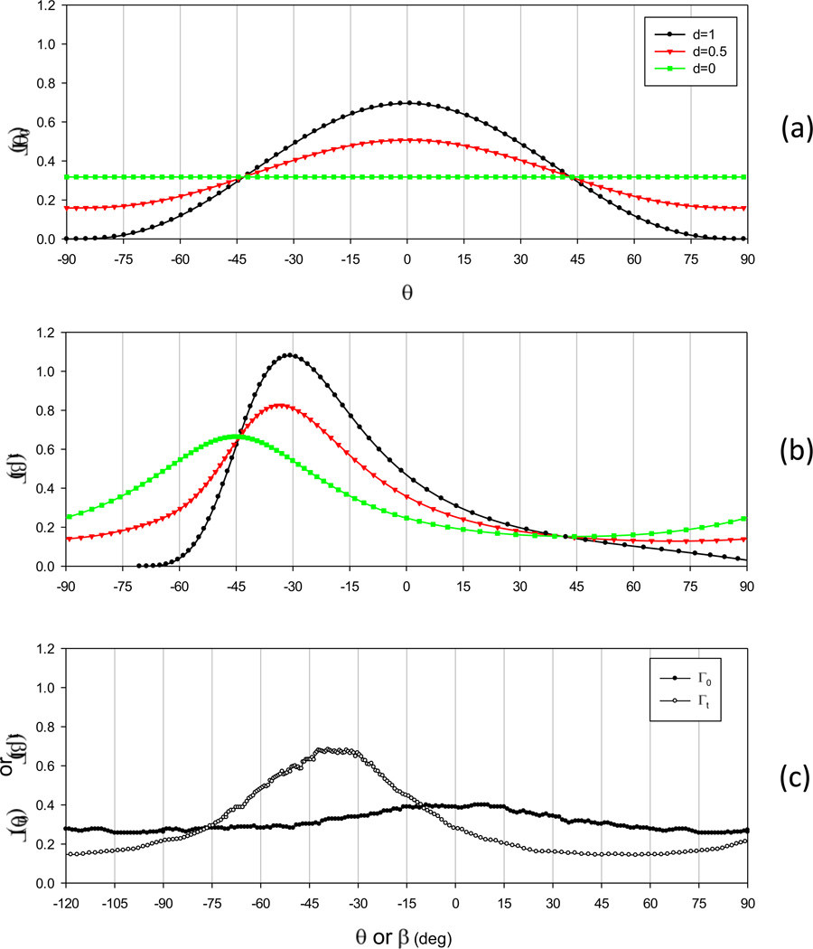
Another interesting aspect of the current study was the apparent resolution of an observed discrepancy in the SALS data in our original 1997 publication (Billiar and Sacks, 1997). In that work, we observed that under strip biaxial stretch the Γ(β) responses were not in good agreement with the experimental results (see Fig. 4 in (Billiar and Sacks, 1997)). At first, this result suggests non-affine deformations; yet the current simulations indicated that when d=0.25 good agreement was obtained (Fig. 7). To investigate this further, we performed affine transformation simulations using equation to determine how the addition of an isotropic oriented fiber phase affects the apparent mean fiber orientation. As the most demanding simulation in the current study we utilized the deformation gradient tensor from the clamped biaxial simulations in the corner region (Fig. 7-b). Using the dispersion of the splay of 30 degrees (typical of bovine pericardium), we observed that increasingly accurate distributions were obtained with smaller d values (Figs. 10-a,b). Next, we remeasured bovine pericardial structure using an upgraded SALS instrument and, unlike in the 1997 study, did not remove the baseline component (Fig. 10-c). When this data was subjected to the same affine deformation, we found a centroid value of ~42°, very close to the ~45° as measured. Note that the estimated value for d in the new bovine pericardial data was 0.2, similar to the 0.25 value used in our simulations (Fig. 5-b).

Figure 10.

Simulations of the effect of an isotropic baseline of a fiber angular distribution functions using the deformation gradient taken from the corner region of the clamped biaxial test in Fig. 7, with d=0, d=0.5 and d=1.0 in the (a) unloaded and (b) loaded configurations. Note in particular note here that as the baseline contribution term d is increased, the centroid of the distribution shifts towards the direction of greatest strain (−45 degrees in this example). (c) Under the same deformation state using pericardial data with the baseline component kept intact, we note that the centroid is now at −42 degrees, very close to the experimentally measured value in Fig. 7 of −45 degrees.

Removal of the baseline component of the SALS signal, as in the original study, was performed at that time since it was unclear whether the baseline contained actual structural information. As a precautionary measure, it was removed as done routinely in small angle x-ray studies (Guinier and Fournet, 1955). Since the time of the 1997 study, we have perfected the SALS technique to validate this procedure for each tissue study and no longer remove this component. While not the final word, these simulations suggest that affine kinematics for pericardial collagenous tissues is a reasonable assumption of the macro level. Moreover, the present results underscore the importance of collecting accurate orientation data in tissue modeling development and application.

4.4 Limitations

In this study, all the simulations were performed based on the assumption that the soft tissue was initially homogenous. However, the pericardium is not homogenous, this can include tissue thickness, fiber orientation, fiber angular distribution, fiber recruitment distribution and fiber volume fraction. We have already have begun to include such information into finite element models (Lee et al., 2013). The structural model presented in this study may be extended to characterize soft tissues with much more complex microstructures, such as multilayers (Stella and Sacks, 2007) and angular variations in structure (Gasser et al., 2012). For example, the strain energy function for fibers may be separated into two forms to model elastin fibers and collagen fibers separately using different fiber angular distribution functions and fiber recruitment functions. Further, variations in fiber properties and structure with orientation are a natural extension. Such model extensions have been contemplated by our group, but for the purposes of the current work we assume constant properties with orientation since applications with constant properties with angular orientation have served as a reasonable approximation.

The key assumption in the structural model is the affine kinematics down to the fiber level. It assumes that the deformation gradient of each fiber and matrix in the RVE are equal to the RVE deformation gradient. There are many reasons that this may not hold at the microlevel, due to such mechanisms as fiber-fiber interaction and fiber-matrix interactions locally. Moreover, most soft tissues have intermediate structures, such as sheets and layers, so that each fiber may not act with complete independence with respect to all other fibers. Additional extensions to this form of modeling that incorporate much more realistic tissue structures may help to further improve simulation accuracy. Moreover, complete 3D implementation of the structural model is currently underway in our laboratory.

4.5 Summary

A structural constitutive model for planar soft tissues was successfully implemented and demonstrated that an isotropic matrix played an essential role in obtaining realistic deformations under uniaxial deformation modes. Numerical simulation also revealed that the preferred fiber orientation in the deformed configuration was strongly related to the initial fiber orientation distribution. By incorporating fiber orientation distribution and fiber recruitment distribution into the strain energy function, the structural model can predict not only the mechanical behavior of soft tissues at the macroscopic scale, but also fiber deformations patterns (in a statistical sense) at the microscopic scale. The new indices introduced herein may be particularly useful in understanding structural adaptations and could easily be used in structural optimization studies in engineered tissue design. Moreover, the present results underscore the importance of architecture in tissue modeling development and application.

Appendix

The total second material elasticity tensor can be written as the sum of the material elasticity tensor of fiber and matrix as

$${\mathrm{ℂ}}^{\mathbf{\text{SE}}}={\mathrm{\varphi }}_{\mathrm{f}}{\mathrm{ℂ}}_{\mathrm{f}}^{\mathbf{\text{SE}}}+{\mathrm{\varphi }}_{\mathrm{m}}{\mathrm{ℂ}}_{\mathrm{m}}^{\mathbf{\text{SE}}}$$ (A1)

The second material elasticity tensor of fiber ${\mathrm{ℂ}}_{\mathrm{f}}^{\mathbf{\text{SE}}}$ is given by

$${\mathrm{ℂ}}_{\mathrm{f}}^{\mathbf{\text{SE}}}={\int }_{-\mathrm{\pi }/2}^{\mathrm{\pi }/2}\mathrm{\Gamma }(\mathrm{\theta })\frac{\partial {\mathrm{S}}_{\text{ens}}}{\partial {\mathrm{E}}_{\text{ens}}}[(\mathbf{N}\otimes \mathbf{N})\otimes (\mathbf{N}\otimes \mathbf{N})]\mathrm{d}\mathrm{\theta }$$ (A2)

The second material elasticity tensor of matrix ${\mathrm{ℂ}}_{\mathrm{m}}^{\mathbf{\text{SE}}}$ is given as

$${\mathrm{ℂ}}_{\mathrm{m}}^{\mathbf{\text{SE}}}=-2\mathrm{\mu }({\tilde{\mathbf{C}}}^{-1}\otimes \frac{\partial {\mathrm{C}}_{33}}{\partial \tilde{\mathbf{C}}}+{\mathrm{C}}_{33}\frac{\partial {\tilde{\mathbf{C}}}^{-1}}{\partial \tilde{\mathbf{C}}})$$ (A3)

Since $\frac{\partial {\mathrm{C}}_{33}}{\partial \tilde{\mathbf{C}}}=-{\mathrm{C}}_{33}{\tilde{\mathbf{C}}}^{-1}$, the second material elasticity tensor of matrix ${\mathrm{ℂ}}_{\mathrm{m}}^{\mathbf{\text{SE}}}$ can be written as

$${\mathrm{ℂ}}_{\mathrm{m}}^{\mathbf{\text{SE}}}=2\mathrm{\mu }{\mathrm{C}}_{33}({\tilde{\mathbf{C}}}^{-1}\otimes {\tilde{\mathbf{C}}}^{-1}-\frac{\partial {\tilde{\mathbf{C}}}^{-1}}{\partial \tilde{\mathbf{C}}})$$ (A4).

Because C̃ is a symmetric tensor, the components of the fourth tensor $\frac{\partial {\tilde{\mathbf{C}}}^{-1}}{\partial \tilde{\mathbf{C}}}$ can be written as

$${\left(\frac{\partial {\tilde{\mathbf{C}}}^{-1}}{\partial \tilde{\mathbf{C}}}\right)}_{\mathrm{i}\mathrm{j}\mathrm{k}\mathrm{l}}=-\frac{1}{2}({\mathrm{C}}_{\mathrm{i}\mathrm{k}}^{-1}{\mathrm{C}}_{\mathrm{j}\mathrm{l}}^{-1}+{\mathrm{C}}_{\mathrm{i}\mathrm{l}}^{-1}{\mathrm{C}}_{\mathrm{j}\mathrm{k}}^{-1})$$ (A5).

The Jaumann stress rate is used for continuum elements and Green-Naghdi stress rate is used for structural elements in ABAQUS/Standard. Therefore, the second material elasticity tensor ℂ^SE = ∂S̃ / ∂Ẽ was related to the corresponding spatial elasticity tensor (Simo and Hughes, 1998) to ensure rapid convergence. During implementation, the following symmetric tangent moduli were used.

$${\mathrm{ℂ}}_{\mathrm{i}\mathrm{j}\mathrm{k}\mathrm{l}}^{\text{UMAT}}={\mathrm{J}}^{-1}{\mathrm{U}}_{\mathrm{i}\mathrm{m}}{\mathrm{U}}_{\mathrm{j}\mathrm{n}}{\mathrm{U}}_{\mathrm{k}\mathrm{p}}{\mathrm{U}}_{\mathrm{l}\mathrm{q}}{\mathrm{ℂ}}_{\mathrm{m}\mathrm{n}\mathrm{p}\mathrm{q}}^{\mathbf{\text{SE}}}+\frac{1}{2}({\tilde{\mathbf{t}}}_{\mathrm{i}\mathrm{k}}{\mathrm{\delta }}_{\mathrm{j}\mathrm{l}}+{\tilde{\mathbf{t}}}_{\mathrm{j}\mathrm{k}}{\mathrm{\delta }}_{\mathrm{i}\mathrm{l}}+{\tilde{\mathbf{t}}}_{\mathrm{i}\mathrm{l}}{\mathrm{\delta }}_{\mathrm{j}\mathrm{k}}+{\tilde{\mathbf{t}}}_{\mathrm{j}\mathrm{l}}{\mathrm{\delta }}_{\mathrm{i}\mathrm{k}})$$ (A6).

REFERENCES

- ABAQUS. Abaqus User Subroutines Reference Manual. 2011. [Google Scholar]
- Beskos DE, Jenkiins JT. A mechanical model for mammalian tendon. Journal of Applied Mechanics. 1975;42:755. [Google Scholar]
- Billiar KL, Sacks MS. A method to quantify the fiber kinematics of planar tissues under biaxial stretch. J Biomech. 1997;30:753–756. doi: 10.1016/s0021-9290(97)00019-5. [DOI] [PubMed] [Google Scholar]
- Billiar KL, Sacks MS. Biaxial mechanical properties of the natural and glutaraldehyde treated aortic valve cusp--Part I: Experimental results. Journal of Biomechanical Engineering. 2000a;122:23–30. doi: 10.1115/1.429624. [DOI] [PubMed] [Google Scholar]
- Billiar KL, Sacks MS. Biaxial mechanical properties of the native and glutaraldehyde-treated aortic valve cusp: Part II--A structural constitutive model. Journal of Biomechanical Engineering. 2000b;122:327–335. doi: 10.1115/1.1287158. [DOI] [PubMed] [Google Scholar]
- Bischoff JE. Continuous versus discrete (invariant) representations of fibrous structure for modeling non-linear anisotropic soft tissue behavior. International Journal of Non-Linear Mechanics. 2006;41:167–179. [Google Scholar]
- Buchanan RM, Sacks MS. Interlayer micromechanics of the aortic heart valve leaflet. Biomech Model Mechanobiol. 2013 doi: 10.1007/s10237-013-0536-6. [DOI] [PMC free article] [PubMed] [Google Scholar]
- Chen H, Liu Y, Slipchenko MN, Zhao X, Cheng JX, Kassab GS. The layered structure of coronary adventitia under mechanical load. Biophys J. 2011;101:2555–2562. doi: 10.1016/j.bpj.2011.10.043. [DOI] [PMC free article] [PubMed] [Google Scholar]
- Cortes DH, Lake SP, Kadlowec JA, Soslowsky LJ, Elliott DM. Characterizing the mechanical contribution of fiber angular distribution in connective tissue: comparison of two modeling approaches. Biomech Model Mechanobiol. 2010;9:651–658. doi: 10.1007/s10237-010-0194-x. [DOI] [PMC free article] [PubMed] [Google Scholar]
- Courtney T, Sacks MS, Stankus J, Guan J, Wagner WR. Design and analysis of tissue engineering scaffolds that mimic soft tissue mechanical anisotropy. Biomaterials. 2006;27:3631–3638. doi: 10.1016/j.biomaterials.2006.02.024. [DOI] [PubMed] [Google Scholar]
- Criscione JC, Sacks MS, Hunter WC. Experimentally tractable, pseudo-elastic constitutive law for biomembranes:I. Theory. J Biomech Eng. 2003;125:94–99. doi: 10.1115/1.1530770. [DOI] [PubMed] [Google Scholar]
- Dafalias YF. Orientation distribution function in non-affine rotations. J Mech Phys Solids. 2001;49:2493–2516. [Google Scholar]
- Driessen NJ, Mol A, Bouten CV, Baaijens FP. Modeling the mechanics of tissue-engineered human heart valve leaflets. J Biomech. 2007;40:325–334. doi: 10.1016/j.jbiomech.2006.01.009. [DOI] [PubMed] [Google Scholar]
- Fata B, Carruthers CA, Gibson G, Watkins SC, Gottlieb D, Mayer JE, Sacks MS. Regional structural and biomechanical alterations of the ovine main pulmonary artery during postnatal growth. J Biomech Eng. 2013;135:021022. doi: 10.1115/1.4023389. [DOI] [PMC free article] [PubMed] [Google Scholar]
- Fata B, Zhang W, Amini R, Sacks M. Insights into Regional Adaptations in the Growing Pulmonary Artery Using a Meso-Scale Structural Model: Effects of Ascending Aorta Impingement. J Biomech Eng. 2014 doi: 10.1115/1.4026457. [DOI] [PMC free article] [PubMed] [Google Scholar]
- Federico S, Gasser TC. Nonlinear elasticity of biological tissues with statistical fibre orientation. J R Soc Interface. 2010;7:955–966. doi: 10.1098/rsif.2009.0502. [DOI] [PMC free article] [PubMed] [Google Scholar]
- Federico S, Grillo A, Giaquinta G, Herzog W. Convex fung-type potentials for biological tissues. Meccanica. 2008;43:279–288. [Google Scholar]
- Freed AD, Einstein DR, Vesely I. Invariant formulation for dispersed transverse isotropy in aortic heart valves: an efficient means for modeling fiber splay. Biomech Model Mechanobiol. 2005;4:100–117. doi: 10.1007/s10237-005-0069-8. [DOI] [PubMed] [Google Scholar]
- Fung YC. Foundations of Solid Mechanics. Englewood Cliffs: Prentice-Hall; 1965. [Google Scholar]
- Fung YC. Biomechanics: Mechanical Properties of Living Tissues. 2nd ed. New York: Springer Verlag; 1993. [Google Scholar]
- Gasser TC, Gallinetti S, Xing X, Forsell C, Swedenborg J, Roy J. Spatial orientation of collagen fibers in the abdominal aortic aneurysm's wall and its relation to wall mechanics. Acta Biomater. 2012;8:3091–3103. doi: 10.1016/j.actbio.2012.04.044. [DOI] [PubMed] [Google Scholar]
- Gasser TC, Ogden RW, Holzapfel GA. Hyperelastic modelling of arterial layers with distributed collagen fibre orientations. J R Soc Interface. 2006;3:15–35. doi: 10.1098/rsif.2005.0073. [DOI] [PMC free article] [PubMed] [Google Scholar]
- Gleason RL, Dye WW, Wilson E, Humphrey JD. Quantification of the mechanical behavior of carotid arteries from wild-type, dystrophin-deficient, and sarcoglycan-delta knockout mice. J Biomech. 2008;41:3213–3218. doi: 10.1016/j.jbiomech.2008.08.012. [DOI] [PMC free article] [PubMed] [Google Scholar]
- Guinier A, Fournet G. Small Angle Scattering of X-Rays. New York: Wiley; 1955. [Google Scholar]
- Hansen L, Wan W, Gleason RL. Microstructurally motivated constitutive modeling of mouse arteries cultured under altered axial stretch. J Biomech Eng. 2009;131:101015. doi: 10.1115/1.3207013. [DOI] [PMC free article] [PubMed] [Google Scholar]
- Hariton I, de Botton G, Gasser TC, Holzapfel GA. Stress-driven collagen fiber remodeling in arterial walls. Biomech Model Mechanobiol. 2007;6:163–175. doi: 10.1007/s10237-006-0049-7. [DOI] [PubMed] [Google Scholar]
- Hollander Y, Durban D, Lu X, Kassab GS, Lanir Y. Experimentally validated microstructural 3D constitutive model of coronary arterial media. J Biomech Eng. 2011;133:031007. doi: 10.1115/1.4003324. [DOI] [PMC free article] [PubMed] [Google Scholar]
- Holzapfel GA, Eberlein R, Wriggers P, Weizascker HW. Large strain analysis of soft biological membranes: Formulatin and finite element analysis. Comput. Methods Appl. Mech. Engrg. 1996;132:45–61. [Google Scholar]
- Holzapfel GA, Gasser TC. A new constitutive framework for arterial wall mechanics and a comparative study of material models. Journal of Elasticity. 2000;61:1–48. [Google Scholar]
- Holzapfel GA, Gasser TC, Ogden RW. Comparison of a multi-layer structural model for arterial walls with a fung-type model, and issues of material stability. J Biomech Eng. 2004;126:264–275. doi: 10.1115/1.1695572. [DOI] [PubMed] [Google Scholar]
- Holzapfel GA, Ogden RW. Constitutive modelling of passive myocardium: a structurally based framework for material characterization. Philos Transact A Math Phys Eng Sci. 2009;367:3445–3475. doi: 10.1098/rsta.2009.0091. [DOI] [PubMed] [Google Scholar]
- Horowitz A, Lanir Y, Yin FC, Perl M, Sheinman I, Strumpf RK. Structural three-dimensional constitutive law for the passive myocardium. J Biomech Eng. 1988;110:200–207. doi: 10.1115/1.3108431. [DOI] [PubMed] [Google Scholar]
- Hughes TJR. The finite element method: linear static and dynamic finite element analysis. Dover Publications; 2000. [Google Scholar]
- Jor JW, Nash MP, Nielsen PM, Hunter PJ. Estimating material parameters of a structurally based constitutive relation for skin mechanics. Biomech Model Mechanobiol. 2011;10:767–778. doi: 10.1007/s10237-010-0272-0. [DOI] [PubMed] [Google Scholar]
- Joyce EM, Moore JJ, Sacks MS. Biomechanics of the fetal membrane prior to mechanical failure: review and implications. Eur J Obstet Gynecol Reprod Biol. 2009;144(Suppl 1):S121–S127. doi: 10.1016/j.ejogrb.2009.02.014. [DOI] [PMC free article] [PubMed] [Google Scholar]
- Kao PH, Lammers S, Tian L, Hunter K, Stenmark KR, Shandas R, Qi HJ. A microstructurally-driven model for pulmonary artery tissue. Journal of biomechanical engineering. 2011;133:051002. doi: 10.1115/1.4002698. [DOI] [PMC free article] [PubMed] [Google Scholar]
- Kenedi RM, Gibson T, Daly CH. Biomechanics and Related Bio-Engineering Topics. In: Kenedi RM, editor. Bioengineering studies of human skin. Oxford: Pergamon Press; 1965. pp. 147–158. [Google Scholar]
- Lake SP, Barocas VH. Mechanical and structural contribution of non-fibrillar matrix in uniaxial tension: a collagen-agarose co-gel model. Annals of biomedical engineering. 2011;39:1891–1903. doi: 10.1007/s10439-011-0298-1. [DOI] [PMC free article] [PubMed] [Google Scholar]
- Lanir Y. A Structural Theory for the Homogeneous Biaxial Stress-Strain Relationships in Flat Collageneous Tissues. Journal of Biomechanics. 1979;12:423–436. doi: 10.1016/0021-9290(79)90027-7. [DOI] [PubMed] [Google Scholar]
- Lanir Y. Constitutive Equations for Fibrous Connective Tissues. journal of biomechanics. 1983;16:1–12. doi: 10.1016/0021-9290(83)90041-6. [DOI] [PubMed] [Google Scholar]
- Lanir Y. Plausibility of structural constitutive equations for isotropic soft tissues in finite static deformations. J. Appl. Mech. 1994;61:695–702. [Google Scholar]
- Lanir Y. Plausibility of structural constitutive equations for swelling tissues--implications of the C-N and S-E conditions. J Biomech Eng. 1996;118:10–16. doi: 10.1115/1.2795935. [DOI] [PubMed] [Google Scholar]
- Lee CH, Amini R, Gorman RC, Gorman JH, 3rd, Sacks MS. An inverse modeling approach for stress estimation in mitral valve anterior leaflet valvuloplasty for in-vivo valvular biomaterial assessment. J Biomech. 2013 doi: 10.1016/j.jbiomech.2013.10.058. [DOI] [PMC free article] [PubMed] [Google Scholar]
- Marsden JE, Hughes TJR. Mathematical Foundations of Elasticity. Dover: Don Mills; 1983. [Google Scholar]
- Mirnajafi A, Raymer J, Scott MJ, Sacks MS. The effects of collagen fiber orientation on the flexural properties of pericardial heterograft biomaterials. Biomaterials. 2005;26:795–804. doi: 10.1016/j.biomaterials.2004.03.004. [DOI] [PubMed] [Google Scholar]
- Mitton R. J Soc Leather Trades' Chem. 29:169–194. [Google Scholar]
- Prot V, Skallerud B, Holzapfel G. Transversely isotropic membrane shells with application to mitral valve mechanics. Constitutive modelling and finite element implementation. Int J Numer Methods Eng. 2007;71:987–1008. [Google Scholar]
- Raghupathy R, Barocas VH. A closed-form structural model of planar fibrous tissue mechanics. J Biomech. 2009;42:1424–1428. doi: 10.1016/j.jbiomech.2009.04.005. [DOI] [PMC free article] [PubMed] [Google Scholar]
- Sacks M. Biaxial mechanical evaluation of planar biological materials. Journal of Elasticity. 2000;61:199–246. [Google Scholar]
- Sacks MS. Incorporation of experimentally-derived fiber orientation into a structural constitutive model for planar collagenous tissues. J Biomech Eng. 2003;125:280–287. doi: 10.1115/1.1544508. [DOI] [PubMed] [Google Scholar]
- Simo JC, Hughes TJR. Computational inelasticity. New York: Springer; 1998. [Google Scholar]
- Soong TT, Huang WN. A stochastic model for biological tissue elasticity in simple elongation. Journal of Biomechanics. 1973;6:451–458. doi: 10.1016/0021-9290(73)90004-3. [DOI] [PubMed] [Google Scholar]
- Spencer A. Deformations of fibre-reinforced materials. Glasgow: Oxford university press; 1972. [Google Scholar]
- Stella JA, Sacks MS. On the biaxial mechanical properties of the layers of the aortic valve leaflet. J Biomech Eng. 2007;129:757–766. doi: 10.1115/1.2768111. [DOI] [PubMed] [Google Scholar]
- Sun W, Sacks MS. Finite element implementation of a generalized Fung-elastic constitutive model for planar soft tissues. Biomech Model Mechanobiol. 2005 doi: 10.1007/s10237-005-0075-x. [DOI] [PubMed] [Google Scholar]
- Sun W, Sacks MS, Sellaro TL, Slaughter WS, Scott MJ. Biaxial mechanical response of bioprosthetic heart valve biomaterials to high in-plane shear. Journal Biomechanical Engineering. 2003;125:372–380. doi: 10.1115/1.1572518. [DOI] [PubMed] [Google Scholar]
- Tong P, Fung YC. The stress-strain relationship for the skin. J Biomech. 1976;9:649–657. doi: 10.1016/0021-9290(76)90107-x. [DOI] [PubMed] [Google Scholar]
- Tonge TK, Voo LM, Nguyen TD. Full-field bulge test for planar anisotropic tissues: part II--a thin shell method for determining material parameters and comparison of two distributed fiber modeling approaches. Acta Biomater. 2013;9:5926–5942. doi: 10.1016/j.actbio.2012.11.034. [DOI] [PubMed] [Google Scholar]
- Truesdell C, Noll W. The Nonlinear Field Theories. In: Flugge S, editor. Handbuch der Physik. Berlin: Springer-Verlag; 1965. pp. 119–126. [Google Scholar]
- Waldman SD, Lee JM. Boundary conditions during biaxial testing of planar connective tissues. Part 1: dynamic behavior. J Mater Sci Mater Med. 2002;13:933–938. doi: 10.1023/a:1019896210320. [DOI] [PubMed] [Google Scholar]
- Waldman SD, Sacks MS, Lee JM. Boundary conditions during biaxial testing of planar connective tissues: Part II: Fiber orientation. Journal of Materials Science Letters. 2002;21:1215–1221. [Google Scholar]
- Wognum S, Schmidt DE, Sacks MS. On the mechanical role of de novo synthesized elastin in the urinary bladder wall. J Biomech Eng. 2009;131:101018. doi: 10.1115/1.4000182. [DOI] [PubMed] [Google Scholar]
- Woo SLY, Seguchi Y. In: Tissue Engineering—1989. BED, editor. New York: Asme; 1989. [Google Scholar]