Quantile Lower Bounds to Population Reliability Based on Locally Optimal Splits

Abstract

Extending the theory of lower bounds to reliability based on splits given by Guttman (1945), this paper introduces quantile lower bound coefficients λ_4(Q) that refer to cumulative proportions of potential locally optimal “split-half” coefficients that are below a particular point Q in the distribution of split-halves based on different partitions of variables into two sets. Interesting quantile values are Q = .05,.50,.95,1.00 with λ_4(.05) ≤ λ_4(.50) ≤ λ_4(.95) ≤ λ_4(1.0). Only the global optimum λ_4(1.0), Guttman’s maximal λ₄, has previously been considered to be interesting, but in small samples it substantially overestimates population reliability ρ. The three coefficients λ_4(.05), λ_4(.50), and λ_4(.95) provide new lower bounds to reliability. The smallest λ_4(.05), provides the most protection against capitalizing on chance associations and thus overestimation, λ_4(.50) is the median of these coefficients, while λ_4(.95) tends to overestimate reliability but also exhibits less bias than previous estimators. Computational theory, algorithm, and publicly available code based in R are provided to compute these coefficients. Simulation studies evaluate the performance of these coefficients and compare them to coefficient alpha and the greatest lower bound under several population reliability structures.

In spite of its controversial nature and despite the availability of newer coefficients with more advantageous properties, coefficient α remains the most widely used descriptor of internal consistency reliability; see e.g., Sijtsma (2009) and discussants. Actually, almost 70 years ago when Guttman (1945) defined his coefficient λ₃, now known as Cronbach’s α, he had already recognized that better lower bounds to reliability were available. One of these, his maximum λ₄ coefficient, is easy to think about conceptually, simply being the largest possible λ₄ coefficient based on two parts that are item composites obtained from an optimal allocation of items to one of two sets. Unfortunately, Guttman provided no way to actually compute his coefficient in practice. Obtaining all possible allocations of items to two sets and computing the associated λ₄ is only feasible with small item sets. With a large number of items, the number of splits to consider may require consideration of trillions of possibilities. In part, this difficulty may explain the absence of λ_4(max) as a practical alternative to coefficient α.

Actually, practical computational methods for λ_4(max) have been proposed, but these appear to have been studied only by their developers. While focusing on computations for the greatest lower bound (glb, ρ₊) to population reliability ρ, Bentler and Woodward (1980) noted that a special case of their computational method would yield λ_4(max). Similarly, Callender and Osburn (1977) and Osburn (2000) provided a recursive partitioning computational methodology for approximating λ_4(max) in small item sets.Osburn’s (2000) results support λ_4(max) as the most consistent and accurate computable lower bound to reliability with population covariance matrices. Nevertheless, the latter authors also made the important point that an estimator λ̂_4(max) might well overestimate reliability in small samples due to capitalization on chance associations arising from data-based allocation of items to one or another of two sets in order to maximize λ₄. These observations provide the motivation for our work. We aim to produce an estimator λ̂_4(1.0) that is consistent for λ_4(max) and also feasible to compute even in large problems, as well as placement of λ̂_4(1.0) into a chain of coefficients λ̂_4(Q) that improve on α̂ while minimizing the chances of overestimation of population reliability ρ in small samples.

When developing a chain of λ₄ coefficients, it is possible to consider two different approaches that define coefficients with different properties. The first approach involves quantiles in the distribution of λ₄ coefficients associated with the entire distribution of possible split halves. In this case every possible split is considered, and the results are summarized with quantile coefficients λ_4[Q]. In practice, due to the increasing computational requirements, larger problems necessitate systematic or randomly sampled points in this distribution. Since many such λ₄ coefficients will be very small and, hence, of no interest in lower-bound reliability estimation, we consider a second approach in which a systematic methodology is used to move away, if possible, from any uninteresting split towards a locally optimal split that yields a greater value of λ₄. For example, there is no justification for keeping items assigned to two sets if a simple move of an item from one set to the other would increase λ₄. If no further simple reassignments increase λ₄, the resulting coefficient represents a locally optimal λ₄ coefficient. The distribution of these locally optimal coefficients is summarized by the quantile coefficients λ_4(Q). While the varying coefficients in a chain will differ in these two approaches, e.g., their minima λ_4[min] and λ_4(min) and other quantile points will be different, their maxima λ_4[max] and λ_4(max) will be the same since both represent the global maximum. This paper addresses only the distribution of locally optimal quantile coefficients λ_4(Q).

The plan of the paper is as follows. A general overview is given in the next section. The subsequent section provides a computational theory for the new coefficients as well as details on implementation. Empirical results observed from three simulation studies follow in the next section. The paper concludes with a discussion.

General Theory and Expectations

While coefficient α (Cronbach, 1951) receives by far the most emphasis in assessment of internal consistency reliability, research has also addressed coefficients that may be better lower bounds to reliability ρ (e.g., Guttman, 1945; Novick & Lewis, 1967; Bentler, 1972; Jackson & Agunwamba, 1977; Woodhouse & Jackson, 1977; Bentler & Woodward, 1980, 1983; ten Berge, Snijders, & Zegers, 1981; Shapiro, 1982). A good recent review is given by Sijtsma (2009) and his various discussants. In general, with the exception of Woodward and Bentler (1978), who provided a “statistical” lower bound to α that would with high probability yield a coefficient not exceeding population reliability, existing coefficients are utilized without concern for whether properties established for a population coefficient also hold in a sample. However, a given coefficient that is an excellent coefficient in a population may be grossly biased for some purposes in medium to small samples. For example, a coefficient that is an unbiased estimator under appropriate conditions cannot be an acceptable lower bound coefficient since it will exceed its population counterpart a substantial amount of the time (half the time if the sampling distribution is unimodal and symmetric). Bias in the sample glb ρ̂₊ and λ̂_4(max) is easy to see when the population covariance matrix is diagonal. In such a case, their population values will be zero, but sample covariances will not all be zero. Then, non-zero common variance exists and, hence, ρ̂₊ > ρ₊; and some allocation of items to two parts will be possible so that λ̂_4(max) > λ_4(max). More generally, ρ̂₊ has been found to exhibit unacceptable overestimation bias in samples less than 1000 (Cronbach, 1988; ten Berge & Sočan, 2004). While research has aimed to provide methods to estimate and correct for this bias (Verhelst, 1998; Shapiro & ten Berge, 2000; Li & Bentler, 2011), this work has not provided a statistical lower-bound to population reliability. Similarly, until a bias corrected method is proposed and validated, coefficient α will remain ubiquitous in circumstances where it may or may not be appropriate. The dominance of α means that other potentially useful estimates for calculating reliability will be ignored (Yuan & Bentler, 2002; ten Berge & Socan, 2004; Sijtsma, 2009; Revelle & Zinbarg, 2009).

Due to the difficulty of constructing an accurate distribution of λ_4(Q) coefficients, in practice the quantiles must be computationally approximated. Although the entire distribution of λ̂_4(Q) may be approximated, in practice only certain points, such as λ̂_4(.05), λ̂_4(.50), and λ̂_4(.95), may be of interest, with λ̂_4(.05) providing the most protection for capitalization on chance, λ̂_4(.50) an intermediate amount, and λ̂_4(.95) providing some minimal protection for large samples. Of course, Guttman (1945) had recommended λ_4(max) as the best possible lower bound; but as noted, previous research (Callender & Osburn, 1977; Osburn, 2000; Yuan & Bentler, 2002; ten Berge & Socan, 2004) can make one doubt the relevance of λ̂_4(max) = λ̂_4(1.0) for small and intermediate sized sample data.

Although the main focus of this paper is on various λ̂_4(Q) coefficients, α̂ and ρ̂₊ are also computed to yield comparative information. Very old results (Cronbach, 1951; Novick & Lewis, 1967) lead one to expect that α̂ should perform well at all sample sizes when the population matrix fits a very restricted 1-factor model with equal factor loadings, but should perform poorly otherwise. Also, ρ̂₊ should perform very well asymptotically, but should be substantially biased at smaller sample sizes. We should expect λ̂_4(1.0) to overestimate population reliability at the smaller sample sizes, but prior research provides no hint on whether λ̂_4(1.0) or ρ̂₊ is liable to be less biased. We expect our various new coefficients to typically outperform α̂. We expect λ̂_4(.05) to perform well generally, especially at the smallest samples sizes. Finally, we expect that λ̂_4(.95) will outperform Guttman’s λ̂_4(1.0), but to be positively biased in all but the largest sample sizes.

Computational Theory

First we give an overview of the computational method that we use to find a candidate coefficient λ̂₄ (or λ₄ with population covariance matrices). A given coefficient or estimate is obtained as the solution to a mathematical minimization problem subject to constraints. As noted by Bentler and Woodward (1980, 1983), such a methodology only finds local minima. In order to locate the global minimum, the procedure is repeated from different random starting positions a large number of times. We recommend use of at least 1000 repetitions, and thus obtainment of a vector of 1000 λ̂₄ estimates. An ordering of these values allows us to obtain λ̂_4(Q) for any quantile values of interest. We take Q = .05, .50, .95, and 1.0.

Function to be Optimized

For optimization purposes, we drop the notational distinction between the population and samples since our methodology works with any covariance matrix. We will let Σ be the p by p (population or sample) covariance matrix to be analyzed. Let t₁ and t₂ be p-vectors of 0 and 1 elements such that t₁+t₂ = 1, a unit-vector. Then, any split-half coefficient can be defined as

$${\lambda }_4=\left(\frac{4\cdot t_1^{\prime }\mathrm{\sum }{t}_2}{{\mathit{1}}^{\prime }\mathrm{\sum }\mathit{1}}\right)=\left(\frac{4t_1^{\prime }\mathrm{\sum }{t}_2}{t_1^{\prime }\mathrm{\sum }{t}_1+t_2^{\prime }\mathrm{\sum }{t}_2+2t_1^{\prime }\mathrm{\sum }{t}_2}\right)=2\left(1-\frac{t_1^{\prime }\mathrm{\sum }{t}_1+t_2^{\prime }\mathrm{\sum }{t}_2}{{\mathit{1}}^{\prime }\mathrm{\sum }\mathit{1}}\right).$$ (1)

There are many such coefficients that depend on whether specific items are assigned to one composite or the other. Obviously, the specific vectors t₁ and t₂ that globally maximize (1) yield λ_4(max) = λ_4(1.0). Rather than work with two different vectors, we relate them to one vector t with +1 and -1 elements where $t_1=\frac{1}{2}(t+\mathit{1})$ and $t_2=\frac{1}{2}(\mathit{1}-\mathit{t})$. Then, we may write (1) as

$${\lambda }_4=1-\frac{t\prime \mathrm{\sum }t}{\mathit{1}\prime \mathrm{\sum }\mathit{1}}=1-\frac{t\prime {\mathrm{\sum }}_{0}t+\mathit{1}\prime {\mathit{D}}_{\mathrm{\sum }}\mathit{1}}{\mathit{1}\prime \mathrm{\sum }\mathit{1}}$$ (2)

where Σ₀ is Σ except that 0s replace it’s diagonal and D_Σ is the diagonal matrix of Σ. From this expression it is clear that maximizing λ₄ is equivalent to minimizing

$$f^{\ast }=t\prime \mathrm{\sum }t=t\prime {\mathrm{\sum }}_{0}t+\mathit{1}\prime {\mathit{D}}_{\mathrm{\sum }}\mathit{1}.$$ (3)

Since the term 1′ D_Σ1 is a constant, namely the sum of the p variances, minimizing f* only requires minimizing t′Σ₀t.

We now provide an approach to optimization that does not require the use of calculus. To do this, we concentrate on a particular element in t and provide a rationale for updating it to its most optimal value (either +1 or -1). Let $t=\left(\begin{array}{c}{t}_i\\ t_{0i}\end{array}\right)$ where i = 1, …, p is an index for variables. The value of t_i is either +1 or -1, and t_0i is the vector of remaining +1 or -1 elements in t. Similarly, let ${\mathrm{\sum }}_0=\left(\begin{array}{cc}0& {\mathrm{\sigma }}_{0i}^{\prime }\\ {\mathrm{\sigma }}_{0i}& {\mathrm{\sum }}_{00}\end{array}\right)$, where the i^th row and column of Σ₀ have been distinguished, i.e., σ_0i is any i^th column not just the first; it excludes the diagonal element. Then, to obtain an optimal λ₄ we need to minimize

$$f=t^{\prime }{\mathrm{\sum }}_{0}t=2t_i{\mathrm{\sigma }}_{0i}^{\prime }{t}_{0i}+t_{0i}^{\prime }{\mathrm{\sum }}_{00}{t}_{0i}.$$ (4)

In this expression the right-most term is constant when considering t_i as an element to be updated and t_0i as constant for the moment. Then it is only necessary to minimize t_iσ_0i′t_0i, since σ_0i ′t_0i can be considered fixed when we want to update t_i only.

To be even more concrete, we introduce a notation that distinguishes between the current values and potential updated values of the vector t. Specifically, we have $t_i^k$ and want to get $t_i^{k+1}$. These are tied to the current function $t_i^k{\mathrm{\sigma }}_{0i}^{\prime }{t}_{0i}^k$ and we want to choose $t_i^{k+1}$ to minimize $t_i^{k+1}{\mathrm{\sigma }}_{0i}^{\prime }{t}_{0i}^k$. That is, for this i^th variable, we want to minimize

$$f_i=t_i^{k+1}{\mathrm{\sigma }}_{0i}^{\prime }{t}_{0i}^k.$$ (5)

The only choices for $t_i^{k+1}$ are +1 and -1. Clearly, f_i will be minimized using the following decision rule:

$$\mathrm{If}{\mathrm{\sigma }}_{0i}^{\prime }{t}_{0i}^k<0\mathrm{then}{t}_i^{k+1}=+1,\mathrm{otherwise}{t}_i^{k+1}=-1.$$ (6)

This update makes the function value $f_i=t_i^{k+1}{\mathrm{\sigma }}_{0i}^{\prime }{t}_{\mathit{oi}}^k$ negative, and provides the basis for our algorithm.

Iterative Algorithm

A systematic way to use the above theory is to

1. Randomly pick a variable i that is in the range 1 to p.

2. Randomly generate a vector t of +1 and -1 elements.

3. Randomly pick an order of j^th elements for the t vector in #2 (j ≠ i), and update each t-value (or not) according to equation (6) until all (p -1) values of t have been updated.

4. Compute λ₄ using the final t from #3 using equations (1) or (2) and save it.

5. Redo Steps 1-4 1000 times, yielding 1000 values of λ₄.

6. Compute the quantile λ₄ values of interest, such as λ_4(.05) ≤ λ_4(.50) ≤ λ_4(.95) ≤ λ_4(1.0).

Steps 1-4 that produce a single estimate of λ₄ produce only a local minimum of functions (1) or (2). The randomized choices in Steps 1-3 are used to avoid reaching the same local minimum whenever these steps are run. An illustration of the monotonic convergence of this algorithm is given in Figure 1, which plots λ̂₄ function values against potential sequential sign changes for 100 runs of Steps 1-4 for an 8-item 2-factor congeneric data structure in a sample of size 320. Each line summarizes the function change or non-change due to Step 6. Minimization with Equations (5) and (6) maximizes λ₄ in Equation (2), which is plotted in the figure. Although the initial λ̂₄ function values range from below .3, all 100 functions increase monotonically to a substantially higher maximum with the largest being near .8.

Figure 1.

Trajectories of 100 randomized starts through 8 iterations of an 8-item two-factor congeneric data structure with n=320.

Because Steps 1-4 are only guaranteed to find local optima, Step 5 is used to create a reasonably large sampling of possible λ₄ values for the Σ being analyzed. Basically, the number of repetitions in Step 5 should be as large as possible, subject to practicality. In the population, the resulting coefficients are computational approximations to true quantile values that could only be obtained with an infinite set of repetitions (instead of 1000) in Step 5. In the analysis of sample data, the algorithm gives computational approximations to sample quantile values. Information about the R implementation of the above optimization methodology is given in the appendix. Additionally, the R package Lambda4, developed by the author, includes the function (Hunt, 2012).

Simulations

A series of three simulation studies was designed to compare the performance of the various new quantile λ̂_4(Q) coefficients to α̂ and ρ̂₊. The glb ρ̂₊ is computed using glb.algebraic (Moltner & Revelle, 2012). The new quantile λ̂_4(Q) coefficients can be calculated using quant.lambda4 (Hunt, 2012) or the code that is included in the appendix. We increased the number of start iterations to 2500 instead of the minimally recommended 1000 in hopes of decreasing the standard deviations in the sampling distributions. The number of variables (items) selected to be studied was taken as sixteen, large enough to be computationally challenging while being small enough to avoid nearing the upper asymptote of 1.0 for the various coefficients.

Procedure

Simulations were conducted in R system for statistical computing (R Development Core Team, 2011) using the psych package (Revelle, 2008). Any given simulation consisted of the following steps: (1) A population covariance structure model was specified with given parameters; (2) A random multivariate normal sample of a given size was obtained from this population, the sample covariance matrix was computed and six internal consistency coefficients were computed from it; (3) Step 2 was repeated 500 times; and (4) Summary statistics based on Step 3 were computed and saved, specifically, for each coefficient, its mean estimate ρ̂, its standard deviation S, and its bias δ = ρ̂ − ρ was computed and saved. Steps 1-4 were repeated for 5 different sample sizes of 50, 100, 400, 1000, and 2000 cases. All of this was repeated for three different population covariance structures.

Population Models and Reliabilities

The first population covariance matrix Σ₁ is based a one-factor model with tau-equivalent items. Factor loadings are all equal to .6 and error variances are set at .6, .7, .8, and .9, repeated 4 times. This is a model setup where coefficient α is known to perform well (Novick, 1966; and Novick & Lewis, 1967; Sijtsma, 2009). The second population covariance matrix Σ₂ is based on two factors. The factor-loading matrix consists of a simple cluster structure (no complex loadings) with equal loadings of .6 and error variances set at .6, .7, .8, and .9, repeated twice for both factors. The factors correlate 0.30. The third population covariance matrix Σ₃ is also based on a factor-loading matrix with a simple cluster structure, but factor loadings vary across items. The loadings repeat with values of .9, .8, .7, and .6 and error variances repeat .6, .7, .8, and .9 across the 16 items, while the factors also correlate 0.30.

The three population covariance structures can be represented as special cases of the confirmatory factor model Σ = ΛΦΛ′ + Ψ. In all three populations, Ψ is a 16×16 diagonal matrix. In Σ₁, Λ is 16×1 and Φ = 1, while in Σ₂ and Σ₃, Λ is 16×2 and Φ is a 2×2 correlation matrix. Population internal consistency reliabilities are defined in all cases as

$$\rho =\frac{\mathit{1}\prime \mathrm{\Lambda \Phi \Lambda }\prime \mathit{1}}{\mathit{1}\prime \mathrm{\sum }\mathit{1}}=1-\frac{\mathit{1}\prime \mathrm{\Psi }\mathit{1}}{\mathit{1}\prime \mathrm{\sum }\mathit{1}}.$$ (7)

The specific values of (7) for the three populations are .9092, .8669, and .9105.

Results

The results for the first population with covariance matrix Σ₁ are shown in Table 1. As shown in the left side of the table, the results are tabulated by sample size (from 50-2000) and within each sample size, the mean estimate ρ̂, the standard deviation S of the estimates, and the mean bias δ = ρ̂ − ρ are reported. The six columns of the table provide these results for each of the six coefficients of interest. The results for populations 2 and 3 based on their covariance matrices Σ₂ and Σ₃ are presented in the same format in Tables 2 and 3, respectively.

Table 1.

One-factor model with equal loadings and ρ = .9092.

Sample Size	λ4(.05)	λ4(.50)	λ4(.95)	λ4(1.00)	ρ+	α
50
ρ̂	0.9099	0.9309	0.9486	0.9585	0.9652	0.9061
S	0.0151	0.0122	0.0098	0.0101	0.0087	0.0202
δ	0.0007	0.0216	0.0393	0.0493	0.0559	-0.0031
100
ρ̂	0.9026	0.9197	0.9352	0.9456	0.9504	0.9065
S	0.0111	0.0095	0.0082	0.0083	0.0077	0.0135
δ	-0.0066	0.0105	0.0260	0.0363	0.0411	-0.0027
400
ρ̂	0.8995	0.9098	0.9195	0.9282	0.9313	0.9088
S	0.0068	0.0062	0.0056	0.0056	0.0053	0.0065
δ	-0.0097	0.0005	0.0102	0.0189	0.0220	-0.0004
1000
ρ̂	0.9027	0.9093	0.9155	0.9215	0.9236	0.9092
S	0.0043	0.0040	0.0037	0.0037	0.0036	0.0040
δ	-0.0065	0.0000	0.0063	0.0122	0.0144	-0.0000
2000
ρ̂	0.9044	0.9090	0.9135	0.9177	0.9192	0.9090
S	0.0032	0.0030	0.0029	0.0030	0.0029	0.0030
δ	-0.0048	-0.0002	0.0042	0.0085	0.0100	-0.0003

Table 2.

Two-factor model with equal loadings and ρ = .8669.

Sample Size	λ4(.05)	λ4(.50)	λ4(.95)	λ4(1.00)	ρ+	α
50
ρ̂	0.8642	0.8957	0.9221	0.9352	0.9465	0.8274
S	0.0259	0.0205	0.0161	0.0155	0.0132	0.0393
δ	-0.0027	0.0288	0.0553	0.0684	0.0796	-0.0395
100
ρ̂	0.8568	0.8819	0.9042	0.9175	0.9254	0.8312
S	0.0186	0.0159	0.0135	0.0131	0.0120	0.0254
δ	-0.0100	0.0150	0.0373	0.0506	0.0585	-0.0357
400
ρ̂	0.8533	0.8683	0.8824	0.8937	0.8976	0.8348
S	0.0105	0.0095	0.0087	0.0085	0.0081	0.0122
δ	-0.0136	0.0014	0.0155	0.0269	0.0307	-0.0320
1000
ρ̂	0.8570	0.8669	0.8760	0.8839	0.8863	0.8351
S	0.0065	0.0060	0.0057	0.0057	0.0055	0.0075
δ	-0.0098	-0.0000	0.0091	0.0171	0.0194	-0.0317
2000
ρ̂	0.8600	0.8669	0.8735	0.8794	0.8810	0.8355
S	0.0048	0.0045	0.0044	0.0044	0.0044	0.0057
δ	-0.0069	0.0000	0.0066	0.0125	0.0142	-0.0313

Table 3.

Two-factor model with unequal loadings and ρ = .9105.

Sample Size	λ4(.05)	λ4(.50)	λ4(.95)	λ4(1.00)	ρ+	α
50
ρ̂	0.9025	0.9257	0.9450	0.9565	0.9650	0.8719
S	0.0171	0.0134	0.0105	0.0100	0.0082	0.0270
δ	-0.0080	0.0152	0.0345	0.0460	0.0544	-0.0386
100
ρ̂	0.8985	0.9168	0.9328	0.9434	0.9499	0.8736
S	0.0146	0.0123	0.0105	0.0102	0.0091	0.0209
δ	-0.0120	0.0063	0.0223	0.0329	0.0394	-0.0369
400
ρ̂	0.8998	0.9101	0.9196	0.9276	0.9314	0.8751
S	0.0077	0.0071	0.0065	0.0061	0.0059	0.0101
δ	-0.0107	-0.0004	0.0091	0.0171	0.0209	-0.0354
1000
ρ̂	0.9019	0.9090	0.9155	0.9211	0.9239	0.8754
S	0.0046	0.0043	0.0041	0.0041	0.0039	0.0059
δ	-0.0086	-0.0015	0.0050	0.0106	0.0134	-0.0351
2000
ρ̂	0.9031	0.9087	0.9136	0.9178	0.9199	0.8756
S	0.0031	0.0030	0.0029	0.0029	0.0027	0.0041
δ	-0.0074	-0.0018	0.0031	0.0073	0.0094	-0.0349

Population 1

It is expected that α̂ will perform well at all sample sizes, and, as shown in the last column of Table 1, this expectation is fulfilled. The mean bias is minimal at all sample sizes. Similarly, λ̂_4(.05) has virtually the same minimal level of bias at all sample sizes. As expected, λ̂_4(1.00) and ρ̂₊ substantially overestimate ρ at all but the largest sample size, with the bias shown by the glb to exceed that of Guttman’s λ̂_4(1.00). While λ̂_4(.95) reduces this bias, the reduction is not as successful as that observed with λ̂_4(.50). Actually, λ̂_4(.50) has much lower bias than ρ̂₊, with λ̂_4(.50) always being an improvement over the glb and having minimal bias when sample size is 100 or greater.

Population 2

On the 2-factor model with equal factor loadings, α̂ can no longer be expected to perform well; and as shown in Table 2, it does not do so. Across various sample sizes, α̂ on average underestimates population reliability by about .03-.04. Both λ̂_4(.05) and λ̂_4(.50) yield a bias that is smaller than that exhibited by α̂ across the various sample sizes; further, this improvement is consistently accomplished with a smaller standard error. There may be a reason to prefer λ̂_4(.05) since it never overestimates ρ on average, while λ̂_4(.50) only avoids overestimation when sample sizes are greater than 400. As in population 1, the maximized coefficients λ̂_4(1.00) and ρ̂₊ always overestimate population reliability, although the positive bias is small when sample size is 1000 or more. As before, the bias of λ̂_4(1.00) is always smaller than that of ρ̂₊. Interestingly, as seen from the S entries, the standard errors of all coefficients are smaller than those obtained by α̂.

Population 3

The results for the 2-factor model with varyingly-sized factor loadings, shown in Table 3, essentially mirror all the results just described for population 2 with its 2-factor model with equal factor loadings. Although the details are important, they need not be repeated.

Discussion

We have presented a theory to extend the idea of Guttman’s λ₄ coefficients to an entire chain of locally optimal quantile-based split-half reliability coefficients λ_4(Q) and provided a computational methodology for obtaining these coefficients in practice. In this initial report on these coefficients, we concentrated on four specific values of Q = .05,.50,.95,1.00 although other values may be worth studying as well. Only the coefficient λ_4(1.00) has previously been considered interesting; and in the population, it is certainly the coefficient we should utilize. However, due to its inherent capitalization on chance associations in sample data, it seemed unlikely to be the best estimated quantile λ̂_4(Q) coefficient to use in practice. Although we were open to the possibility that λ̂_4(.05) or λ̂_4(.95) might perform better in practice than λ̂_4(.50), a priori we leaned toward the latter coefficient as a moderate member of the λ_4(Q) chain. The generally best performing lower bound λ̂_4(Q) coefficient in our simulations with covariance matrices of order 16 is λ̂_4(.05). Not only did this coefficient come to within about .01 of the population reliability on average under various model structures and sample sizes, it had the virtue of essentially never overestimating population reliability.¹ In contrast, in the more realistic multiple factor population models, coefficient α̂ substantially underestimated population reliability in general. On the other hand, one of the recently recommended alternatives to α̂, namely ρ̂₊, the greatest lower bound (see Jackson & Agunwamba, 1977; Bentler & Woodward, 1980, 1983), essentially always overestimated population reliability. While Guttman’s (1945) maximal λ̂_4(1.00) did yield less overestimation than that by ρ̂₊, the degree of overestimation of reliability was still substantial and unacceptable at all but the largest sample sizes. As far as we can tell, the proposed methodology is the first in about 35 years to be concerned with obtaining a sample-based lower bound to population reliability. Although our proposed approach is promising as we have shown, other approaches to the development of statistical lower bounds to population reliability should be considered. Future research can be directed at obtaining confidence intervals for our Lambda4 coefficients and adapting these to lower bound estimation of population reliability as demonstrated by Woodward and Bentler (1978). Confidence intervals and hypothesis testing techniques available for other estimators of population reliability (Feldt, Woodruff, & Salih, 1987; Raykov & Shrout, 2002; Raykov 2002; Maydeu-Olivares, Coffman, & Hartmann 2007) also could be adapted to obtaining statistical lower bounds to population reliability. Such work will be considered elsewhere.

The statistical basis of our approach is that sample quantiles are known to be consistent estimators of their population counterparts. We relied naively on λ̂_4(Q) ≤ λ̂_4(1.0), especially for small values of Q, but in future work we could use a specialized bootstrap approach (Chatterjee, 2011) to obtain the standard error of λ̂_4(1.0) and adapt Woodward and Bentler’s (1978) method to provide a probabilistic quantile lower bound. The choice of probability level with which λ̂_4(1.0) ≤ λ_4(1.0) would, of course, remain subjective.

A drawback to the practical use of lower bound λ̂_4(Q) coefficients as currently proposed is that the choice of the specific value of Q to use in any particular situation is somewhat arbitrary. Based on our research, Q=.05 is a good value; but as noted by a reviewer, another value such as .01 or .07 also might work well, with smaller values being more appropriate for smaller samples to minimize the effect of chance associations in smaller sample sizes. Nevertheless, as the sample size increases, the distribution of the Q coefficients becomes more leptokurtic and the quantiles converge to very similar estimates of reliability (see Tables 1, 2, and 3). An advantage of λ̂_4(.05) as shown in the tables is that it is hardly affected by sample size. At this point, we would feel comfortable to report λ_4(.05) if it is a good bit larger than α̂ since, if there is any overestimation in λ̂_4(.05), it will be much less than that exhibited by its alternatives, such as the frequently recommended glb.

It should be recognized that our approach to computation of λ_4(Q) coefficients is not that of a simple global optimization problem. Use of global optimization or approximate global optimization methods would be appropriate when one is interested only in λ_4(1.0), and then many methods become available (e.g., in psychometrics, Brusco, Singh, & Steinley, 2009; in the optimization literature, Wolsey, 1998, and Floudas & Gounaris, 2009). However, we seek to define a distribution of locally maximized λ₄ coefficients. Our combination of randomized initial splits with local optimization is an effective approach to finding the quantiles in the distribution of local maxima. The random restarts are designed to provide samples from that distribution. As illustrated at the starting points of Figure 1, random starts will encounter very low values of λ₄ that no reliability theorist would consider for use as a lower bound to reliability. The subsequent local minimization fairly quickly finds better solutions in the neighborhood of these start values if they exist.

Although computations involving quantile λ_4(Q) coefficients are heavy compared to the computation of coefficient α, these computations are trivial on current computer systems and promise to become even more trivial in the future. Nonetheless, it has to be acknowledged that as the number of variables increases, the size of the potential pool of split-half coefficients increases exponentially; and it will be increasingly difficult to be sure that the chosen quantiles in the distribution of λ_4(Q) coefficients can be computed with enough precision. In practice, this may mean that the number of random restarts of our iterative algorithm needs to be increased when working with a very large covariance matrix. With a large number of items the computation time in R will increase, so cursory testing is recommended to determine the stability of the estimates. Further code development in faster languages such as Fortran or C could render computation speed concerns unwarranted. If one chooses to use 1000 iterations the distribution may not be as symmetrical or smooth; but, as seen in seen in Figures 2, 3, and 4,² the distributional qualities are similar. This issue is outside the scope of the current paper, but clearly research is needed to make meaningful empirically-based recommendations in this regard.

Figure 2.

Frequency distribution from 10000 repetitions of Algorithm Step 5.

Figure 3.

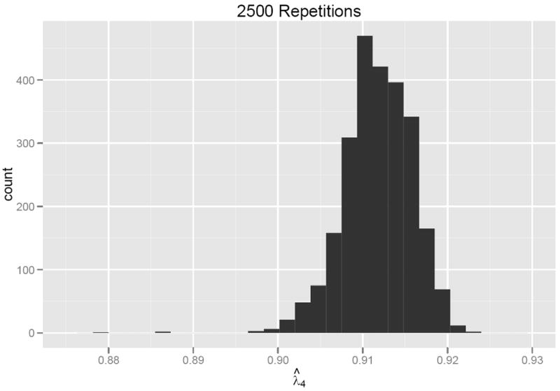
Frequency distribution from 2500 repetitions of Algorithm Step 5.

Figure 4.

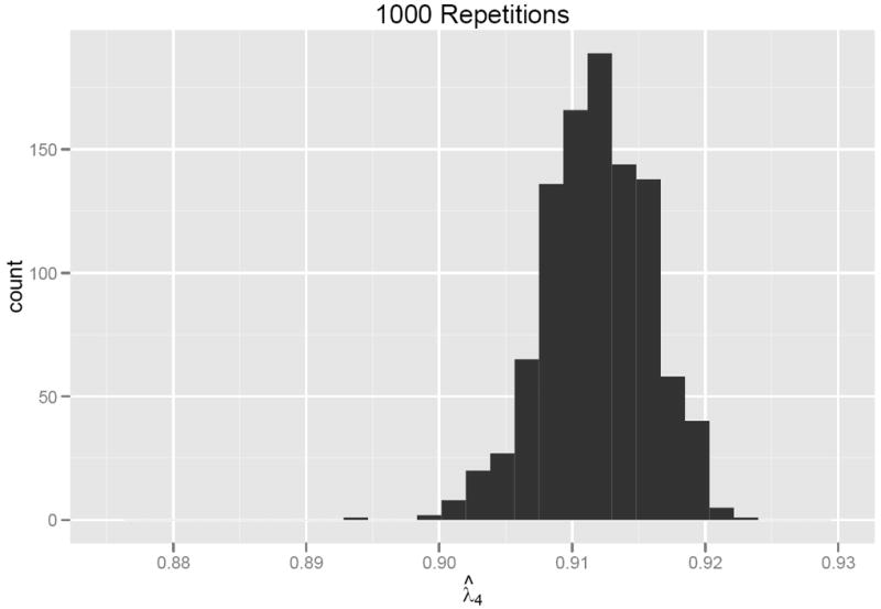
Frequency distribution from 1000 repetitions of Algorithm Step 5.

The theoretical and empirical research described above is quite encouraging with regards to the use of λ̂_4(Q) coefficients in practice. Of course, the limited simulations done in this report need to be augmented with further research under a greater variety of population structures, loading and unique variance parameters, distributional conditions, and with a widely varying number of items in order to evaluate whether the conclusions from this research generalize to such wider contexts. Furthermore, this paper has only studied the usefulness of locally optimal λ_4(Q) coefficients. It would be worthwhile to evaluate the usefulness of quantiles of split-half λ_4[Q] coefficients that describe the entire distribution of λ₄ coefficients. Values that achieve good lower bound properties will no doubt be different from those found here. For example, the median value λ_4[.50] should be comparable to coefficient α which, under narrow circumstances, is the mean of all (population) split half reliabilities (Cronbach, 1951; Novick & Lewis, 1967).³ To improve on α with λ_4[Q] coefficients most likely will require Q > 0.50. Issues such as this are the focus of our ongoing further research.

Appendix

R Implementation for Computation of Various λ_4(Q) Coefficients

quant.lambda4<-function(x, starts=1000, quantile=.5, show.lambda4s=FALSE) {
l4.vect<-rep(NA, starts)
#Determines if x is a covariance or data matrix and establishes a covariance matrix for estimation.
p <- dim(x)[2]
if (dim(x)[1] == p) sigma <- as.matrix(x) else sigma <- var(x, use=“pairwise”)
items<-ncol(sigma)
#Creates an empty matrix for the minimized tvectors
splitmtrx<-matrix(NA, nrow=items, ncol=starts)
# creates the row and column vectors of 1s for the lambda4 equation.
onerow<-rep(1,items)
onerow<-t(onerow)
onevector<-t(onerow)
f<-rep(NA,starts)
for(y in 1:starts) {
#Random number generator for the t-vectors
trow<-(round(runif(items, min=0, max=1))-.5)*2
trow<-t(trow)
tvector<-t(trow)
#Creating t vector and row
tk1<-(tvector)
tk1t<-t(tk1)
tk2<-(trow)
tk2t<-t(tk2)
#Decision rule that determines which split each item should be on. Thus minimizing the numerator.
sigma0<-sigma
diag(sigma0)<-0
random.order<-sample(1:items)
for (o in 1:items) {
oi<-sigma0 [, random.order [o]]
fi<-oi%*%tk1
if (fi < 0) {tk1 [random.order [o] , 1] <- 1}
if (fi >= 0) {tk1 [random.order [o] , 1]<- -1}
}
t1<- (1/2) * (tk1+1)
fk1 <-tk1t%*%sigma0%*%tk1
t1t<-t (t1)
t2<-(1-t1)
t2t<- t(t2)
f [y]=fk1
splitmtrx [,y]<-t1
l4.vect[y]<-(4*(t1t%*%sigma%*%t2)) / (onerow%*%sigma%*%onevector)
}
quants<-quantile (l4.vect, quantile)
lambda4.quantile=quants
if (show.lambda4s==FALSE) {
result<-list (lambda4.quantile=lambda4.quantile)
}
if(show.lambda4s==TRUE) {
result<-list (lambda4.quantile=lambda4.quantile, l4.vect=l4.vect)
}
return (result)
}
#Example computation
quant.lambda4 (USJudgeRatings, starts=2500, quantile=c(.05, .5, .95))
$lambda4.quantile
5% 50% 95%
0.9772899 0.9846840 0.9902834
$lambda4.optimal
[1] 0.9919463

References

- Bentler PM. A lower-bound method for the dimension-free measurement of internal consistency. Social Science Research. 1972;1:343–357. [Google Scholar]
- Bentler PM, Woodward JA. Inequalities among lower bounds to reliability: With applications to test construction and factor analysis. Psychometrika. 1980;45:249–267. [Google Scholar]
- Bentler PM, Woodward JA. The greatest lower bound to reliability. In: Wainer H, Messick S, editors. Principals of modern psychological measurement: A Festschrift for Frederic M Lord. Hillsdale, NJ: Erlbaum; 1983. pp. 237–253. [Google Scholar]
- Brusco MJ, Singh R, Steinley D. Variable neighborhood search heuristics for selecting a subset of variables in principal component analysis. Psychometrika. 2009;74:705–726. [Google Scholar]
- Callender JC, Osburn HG. A method for maximizing split-half reliability coefficients. Educational & Psychological Measurement. 1977;37:819–826. [Google Scholar]
- Chatterjee A. Asymptotic properties of sample quantiles from a finite population. Annals of the Institute of Statistical Mathematics. 2011;63:157–179. [Google Scholar]
- Cronbach LJ. Coefficient alpha and the internal structure of tests. Psychometrika. 1951;16:297–334. [Google Scholar]
- Cronbach LJ. Internal consistency of tests: Analyses old and new. Psychometrika. 1988;53:63–70. [Google Scholar]
- Feldt LS, Woodruff DJ, Salih FA. Statistical inference for coefficient alpha. Applied Psychological Measurement. 1987;11(1):93–103. [Google Scholar]
- Floudas CA, Gounaris CE. A review of recent advances in global optimization. Journal of Global Optimization. 2009;45:3–38. [Google Scholar]
- Guttman LA. A basis for analyzing test-retest reliability. Psychometrika. 1945;10:255–282. doi: 10.1007/BF02288892. [DOI] [PubMed] [Google Scholar]
- Hunt T. Lambda4: Estimation techniques for the reliability estimate: Maximized Lambda4. R package version 2.0. 2012 URL http://cran.r-project.org/web/packages/Lambda4/index.html.
- Jackson PH. A note on the relation between coefficient alpha and Guttman’s “split-half” lower bounds. Psychometrika. 1979;44:251–252. [Google Scholar]
- Jackson PH, Agunwamba CC. Lower bounds for the reliability of the total score on a test composed of non-homogeneous items: I. Algebraic lower bounds. Psychometrika. 1977;42:567–578. [Google Scholar]
- Li L, Bentler PM. The greatest lower bound to reliability: Corrected and resampling estimators. Modeling and Data Analysis. 2011;1:87–104. [Google Scholar]
- Moltner A, Revelle W. glb.algebraic {psych}. Find the greatest lower bound to reliability. R Graphical Manual. 2012 http://rgm2.lab.nig.ac.jp/RGM2/func.php?rd_id=psych:glb.algebraic.
- Novick MR. The axioms and principal results of classical test theory. Journal of Mathematical Psychology. 1966;3:1–18. [Google Scholar]
- Novick MR, Lewis CL. Coefficient alpha and the reliability of measurements. Psychometrika. 1967;32:1–13. doi: 10.1007/BF02289400. [DOI] [PubMed] [Google Scholar]
- Osburn HG. Coefficient alpha and related internal consistency reliability coefficients. Psychological Methods. 2000;5:343–355. doi: 10.1037/1082-989x.5.3.343. [DOI] [PubMed] [Google Scholar]
- Raykov T. Analytic estimation of standard error and confidence interval for scale reliability. Multivariate Behavioral Research. 2002;37(1):89–103. doi: 10.1207/S15327906MBR3701_04. [DOI] [PubMed] [Google Scholar]
- Raykov T, Shrout PE. Reliability of scales with general structure: Point and interval estimation using a structural equation modeling approach. Structural Equation Modeling. 2002;9(2):195–212. [Google Scholar]
- R Development Core Team. R: A language and environment for statistical computing. R Foundation for Statistical Computing; Vienna, Austria: 2011. http://www.R-project.org. [Google Scholar]
- Revelle W. psych: Procedures for psychological, psychometric, and personality research. R package version 1.0-51. 2008 URL http://cran.r-project.org/web/packages/psych/index.html.
- Revelle W, Zinbarg RE. Coefficients alpha, beta, omega, and the glb: Comments on Sijtsma. Psychometrika. 2009;74(1):145–154. [Google Scholar]
- Shapiro A. Rank reducibility of a symmetric matrix and sampling theory of minimum trace factor analysis. Psychometrika. 1982;47:187–199. [Google Scholar]
- Shapiro A, ten Berge JMF. The asymptotic bias of minimum trace factor analysis, with applications to the greatest lower bound to reliability. Psychometrika. 2000;65:413–425. [Google Scholar]
- Sijtsma K. On the use, the misuse, and the very limited usefulness of Cronbach’s alpha. Psychometrika. 2009;65:23–28. doi: 10.1007/s11336-008-9101-0. [DOI] [PMC free article] [PubMed] [Google Scholar]
- ten Berge JMF, Snijders TAB, Zegers FE. Computational aspects of the greatest lower bound to reliability and constrained minimum trace factor analysis. Psychometrika. 1981;46:201–213. [Google Scholar]
- ten Berge JMF, Sočan G. The greatest lower bound to the reliability of a test and the hypothesis of unidimensionality. Psychometrika. 2004;69:613–625. [Google Scholar]
- Verhelst ND. Estimating the reliability of a test from a single test administration. Arnhem: CITO; 1998. Measurement and Research Department Report No. 98-2. [Google Scholar]
- Wolsey LA. Integer programming. New York: Wiley; 1998. [Google Scholar]
- Woodhouse B, Jackson PH. Lower bounds for the reliability of a test composed of nonhomogeneous items II: A search procedure to locate the greatest lower bound. Psychometrika. 1977;42:579–591. [Google Scholar]
- Woodward JA, Bentler PM. A statistical lower-bound to population reliability. Psychological Bulletin. 1978;85:1323–1326. [PubMed] [Google Scholar]
- Yuan KH, Bentler P. On the robustness of the normal-theory based asymptotic distributions of three reliability coefficient estimates. Psychometrika. 2002;67(2):251–259. [Google Scholar]