Empirical Bayes Correction for the Winner's Curse in Genetic Association Studies

Abstract

We consider an Empirical Bayes method to correct for the Winner's Curse phenomenon in genome-wide association studies. Our method utilizes the collective distribution of all odds ratios (ORs) to determine the appropriate correction for a particular single-nucleotide polymorphism (SNP). We can show that this approach is squared error optimal provided that this collective distribution is accurately estimated in its tails. To improve the performance when correcting the OR estimates for the most highly associated SNPs, we develop a second estimator that adaptively combines the Empirical Bayes estimator with a previously considered Conditional Likelihood estimator. The applications of these methods to both simulated and real data suggest improved performance in reducing selection bias.

Introduction

For the past 7 years, hundreds of disease-associated genetic variants have been identified via genome-wide association studies (GWAS), where very large cohorts of disease cases and controls are simultaneously genotyped at hundreds of thousands of markers [Wang et al., 2005]. Typically, the analysis of the resulting data set involves testing many hypotheses, each looking for the presence of disease association at a single variant. Stringent multiple hypothesis testing corrections are normally used to ensure that the subset of the variants that will be investigated with the follow-up study (for instance, fine-mapping studies or molecular function studies) has few false positive signals. While the selection of only these significant single-nucleotide polymorphisms (SNPs) does reduce the proportion of false positives that are followed up, it also leads to a bias—in that the raw-estimated odds ratios (ORs) associated with the selected SNPs represent far more extreme deviations from the null hypothesis (i.e., an OR of 1) compared to the true ORs. This selection bias has been described as the “Winner's Curse” [Capen et al., 1971]. Numerous attempts have been made to correct it in GWAS settings as detailed below.

The problem was first addressed in Zollner and Pritchard [2007], who noted that the estimated probabilities of disease for each of the three genotypes (i.e., penetrance parameters) for the most highly associated SNPs are typically biased in a genome-wide scan. To correct for this bias, the authors suggested maximizing a likelihood conditional on the selection rule, in place of a regular likelihood. Since then, most work has focused on correcting the estimated OR, instead of the estimated penetrance parameters. As Zhong and Prentice [2008] mentioned, the estimation of the OR has received special attention in epidemiologic studies since it can be conveniently and consistently estimated by using techniques such as logistic regression, whereas estimating the penetrance requires a prior, out of sample, estimate of disease prevalance. An approach, that is computationally convenient and relatively simple, focuses on first standardizing the raw-estimated log odds ratio (log-OR) for each SNP (e.g., Xiao and Boehnke [2009, 2011], Zhong and Prentice [2008, 2010], and Ghosh et al. [2008]). In this approach, we compute:

$$Z_i=\frac{{\widehat{\beta }}_i}{SE({\widehat{\beta }}_i)},$$ (1)

where β̂_i is the estimated log-OR for the ith SNP (1 ≤ i ≤ N) and SE(β̂_i) is its standard error. (Note that in this manuscript we denote random variables in uppercase and their realized values in lowercase.) It is assumed $Z_i\stackrel{approx}{\sim }N({\mu }_i,1)$ and that SNPs are selected according to their associated Z-scores being larger than some threshold C in absolute value. For SNP i, with Z_i = z_i, the Conditional Likelihood function is defined as: L_c(μ_i) = φ(z_i − μ_i)/(Φ(−c + μ_i) + Φ(−c − μ_i)), where $\phi (z)=\frac{1}{\sqrt{2\pi }}{e}^{-\frac{z^2}{2}}$ and $\mathrm{\Phi }(z)={\int }_{-\infty }^z\phi (t)\mathrm{d}t$ for −∞ < μ_i < ∞. This is the conditional density of Z_i ∼ N(μ_i, 1), at z given the event {|Z_i| > C}. Typically $C={\mathrm{\Phi }}^{-1}(1-\frac{\alpha }{2})$, where α is a Bonferonicorrected significance level. This can be used to define various estimators of μ_i, via manipulation of this function. While using the Conditional Likelihood to correct the bias in the estimated log-ORs is a nice idea and does work, it can be suboptimal, since it processes each SNP marginally and hence ignores information that can be borrowed by looking at the set {z_i: i ≤ N} collectively. To see that we might be able to improve the estimation of a particular log-OR by using the Z-scores from the other SNPs, it is useful to first imagine we knew the empirical distribution of the “true” log-ORs over the hundreds of thousands of SNPs. For concreteness, we will consider two cases, as shown in Fig. 1. In the first case, represented by the upper panel, we assume that the distribution of the nonzero true log-ORs is normal. Under this assumption, if the largest estimated log-OR falls well outside the effective support of this distribution (as is indicated by the red cross), it is clear that one should shrink this estimated log-OR significantly. The lower panel represents a scenario where we know that there are three very important SNPs, indicated by asterixes, having true log-ORs far larger than the majority of associated SNPs. The largest estimated log-OR is in the vicinity of the hypothesized true log-ORs for these three SNPs. In this case, one might consider the largest estimated log-OR, represented by a red cross, as not being biased since we would a priori have expected the three important SNPs to have produced large estimated log-ORs of similar size (Fig. 1). The point being emphasized here is that the way we adjust the estimated log-ORs should depend on the distribution of the true log-OR when we know this distribution. In addition, information about the distribution of the true log-ORs is encoded in the empirical distribution {z_i:i ≤ N}. The Conditional Likelihood methods, which consider each SNP marginally, do not use the information in this empirical distribution and as a result can be inefficient.

Figure 1.

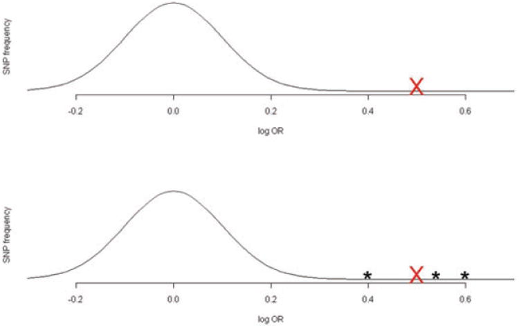
In the upper panel, the normal curve represents a hypothetical distribution of the true log-ORs of disease association for all SNPs on a genome-wide association platform. The lower panel represents an alternative scenario where there are 3 “outlier” SNPs with extremely large population level log-ORs, with the other log-ORs again following a normal distribution. In both scenarios, the largest estimated log-OR is represented by the red cross. It is intuitively clear that it is more appropriate to shrink the estimated OR in the first scenario compared to the second.

Methods

Our set up will follow [Zhong and Prentice, 2008] and others in that we will work with standardized log-ORs defined by $Z_i=\frac{{\widehat{\beta }}_i}{SE({\widehat{\beta }}_i)}$, see (1). Asymptotically, Z_i ∼ N(μ_i, 1), where μ_i = 0 if there is no association between that SNP and disease. Consider the true, but unknown distribution of the SNP-effects, {μ_i: i ≤ N}, for the particular disease of interest. We can conceptualize this distribution with a continuous density function, f, and regard the true standardized log-OR for a particular SNP, i, as a random draw, μ_i ∼ f, from this density. (In fact, we only assume a continuous density for ease of exposition—the squared error optimality explained below also holds for discrete f.) Note while there are a finite number of SNPs genotyped as part of the scan, this number is generally large enough in genome-wide association settings to think of the distribution of the true log-ORs over all SNPs as approximately continuous, with a possibly heavy concentration of mass very near zero. Our idea then is to use this true distribution f(μ) as a prior density, and use the resulting posterior mean as the corrected log-OR.

Squared Error Loss Optimality of Bayesian Shrinkage When f is Known

Here, we demonstrate optimality of the posterior mean for μ_i, E(μ_i|z_i) given Z_i = z_i, under squared error loss, when f, defined as above, is used as the prior distribution. (For brevity, we refer to E(μ_i|z_i) as simply “the posterior mean” in what follows.) This result is not new, and can be viewed as an application of the standard result from statistical decision theory that a Bayes estimator will minimize the Bayes risk over the class of all estimators for a particular prior distribution [Berger, 1985]. However, sketching a proof for this result restricted to our specific setting of correcting selection bias in GWAS is useful for intuition. Note first that there exists a random vector (Z_i, μ_i) corresponding to each SNP, i ≤ N, where μ_i can be thought of as a latent random draw from the distribution f and the observed random variable Z_i is generated conditional on μ_i using Z_i | μ_i ∼ N(μ_i, 1). Since the aforementioned process is assumed to take place independently for each SNP i, we can remove the subscripts i from μ and Z in the following discussion. Now consider, for a given SNP, the set of functions δ: ℝ → ℝ of the Z-score, Z, which represent estimators for the mean, μ, corresponding to that SNP. We would like to choose δ to minimize the average squared error loss over all SNPs. That is, we would like to find the δ̂ so that

$$\begin{array}{c}\widehat{\delta }={argmin}_{\delta }\left\{\frac{1}{N}\sum _{i=1}^N{E}_{Z_i|{\mu }_i}{(({\mu }_i-\delta (Z_i))}^2\right\}\\ \sim {argmin}_{\delta }\{{\int }_{-\infty }^{\infty }{E}_{Z|\mu }{((\mu -\delta (Z))}^{2}f(\mu )\mathrm{d}\mu \}\\ ={argmin}_{\delta }\left\{{\int }_{-\infty }^{\infty }\right({\int }_{-\infty }^{\infty }{(\mu -\delta (z))}^2\phi (z-\mu )\mathrm{d}z)f(\mu )\mathrm{d}\mu \}.\end{array}$$ (2)

Note that the right-hand side of the first equality in the above equation can be thought of as the expectation of E_Z|μ((μ – δ(Z))² with respect to the empirical distribution: {μ_i: i ≤ N}, which is then approximated with the continuous density f Letting p(z) denote ${\int }_{-\infty }^{+\infty }f(\mu )\phi (z-\mu )\mathrm{d}\mu$, that is the marginal distribution of Z at z from Fubini's theorem (valid so long as (2) is finite, see Dudley, 2002) it follows that we can rewrite φ(z − μ)f(μ) = p(z)f(μ | z), where f(μ| z) is the posterior distribution of μ given Z = z, and change the order of integration in (2) so that

$$\widehat{\delta }={argmin}_{\delta }{\int }_{-\infty }^{\infty }\{{\int }_{-\infty }^{\infty }{(\mu -\delta (z))}^{2}f(\mu |z)\mathrm{d}\mu \}p(z)\mathrm{d}z.$$ (3)

Noting that the posterior mean minimizes the expression in braces for each value of z

$$E(\mu |z)={argmin}_{\delta }{\int }_{-\infty }^{\infty }{(\mu -\delta (z))}^{2}f(\mu |z)\mathrm{d}\mu ,$$ (4)

it follows that δ̂(z)= E (μ | z). Note that a similar argument demonstrates the optimality of the posterior mean under selection. For instance, if only SNPs such that |Z_i| ≥ C were selected, the analogue equation for (2) would be:

$$\widehat{\delta }={argmin}_{\delta }{\int }_{-\infty }^{\infty }\left[{\int }_{|z|>C}{(\mu -\delta (z))}^2\frac{\phi (z-\mu )}{P\{|Z|>C|\mu \}}\right]\mathrm{d}zP\times \{|Z|>C|\mu \}f(\mu )\mathrm{d}\mu ,$$ (5)

noting that the terms P{|Z| > C| μ} cancel in the numerator and denominator of this expression, and again that one can rewrite φ(z − μ)f(μ) as p(z)f(μ | z), it follows that

$$\widehat{\delta }={argmin}_{\delta }{\int }_{-C}^{\infty }\{{\int }_{-\infty }^{\infty }{(\mu -\delta (z))}^{2}f(\mu |z)\mathrm{d}\mu \}p(z)\mathrm{d}z,$$ (6)

which by the same argument as above is minimized by the posterior mean. A similar argument can be used for other selection rules (where P{|Z| > C|μ} would be replaced by P{Z ∈ S | μ}, for selecting Z in a set).

Empirical Bayes Estimation When f(μ) is Unknown

Unfortunately, investigators can only make an educated guess about the form of the desntiy f, so it seems at first that the above result is not usable in practice. However, recently Efron [2011] has investigated an Empirical Bayes alternative to E(μ | z), motivated by “Tweedie's formula,” which expresses the posterior mean and variance in terms of the marginal density function, p(z). While Tweedie's formula applies over general canonical exponential families, there is a particularly nice form for the posterior mean and posterior variance for μ given Z= z in the case of normally distributed unit variance Z, as shown below:

$$E(\mu |z)=z+\frac{\mathrm{d}}{\mathrm{d}z}logp(z).$$ (7)

$$Var(\mu |z)=1+\frac{{\mathrm{d}}^2}{{\mathrm{d}z}^2}logp(z).$$ (8)

The advantage of expressing the posterior mean in this form is that we can directly use the empirical density of the Z-scores in estimating (7). As in Efron [2009], we estimate log p using the following two steps:

1. Define bins B₁,…, B_b which together form an equally spaced partition of the interval [min{z₁,…, z_N}, max{z₁, …, z_N}]. Let us assume that the counts of the number of Zs falling within the bins are {C₁,…, C_b} and that the bin midpoints are {m₁, …, m_b}.

2. Regress the bin counts against a set of natural spline basis functions with knots at the bin-midpoints, and 7degrees of freedom, using a Poisson generalized linear model. The fitted regression function at z is an estimate of log p(z), up to proportionality.

Here, we modify Efron's approach slightly by selecting the number of basis functions (or equivalently degrees of freedom) for the natural spline to minimize the Bayesian Information Criterion (BIC) for the Poisson regresion model. The effect of using some model selection is that the estimated density will generally have a greater degree of local curvature when the bin counts are large (or equivalently N is very large) than when N is small, reflecting the fact that local features of the marginal density can be reliably estimated when the number of SNPs is large. The results are quite insensitive to the choice of the number of bins, b, so long as b is reasonably large (see Supporting Information Fig. S1 for a sensitivity analysis with respect to b); here, we use b = 120, the same value as Efron assumed. Having estimated log p(z), it is straight forward to derive an estimate of the posterior mean, $\widehat{E}(\mu |z)=z+\frac{\mathrm{d}}{\mathrm{d}z}log\widehat{p}(z)$, by numerical differentiation as in (7).

Bayesian Confidence Intervals for the log-OR

Assuming approximate normality of the posterior distribution, it is natural to use (8) to derive approximate Bayesian confidence intervals for μ_i using $\widehat{E}(\mu |z_i)\pm z_{\alpha /2}\sqrt{\widehat{\mathrm{V}}\text{ar}(\mu |z_i)}$, i ≤ N, where z_α/2 is the 100(1 − α/2)% percentile of the standard normal distribution. However, this formula ignores the estimation error that occurs in estimating the posterior mean, which is given by $Var(\frac{\mathrm{d}}{\mathrm{d}z}log\widehat{p}(z_i))$, where p̂(z_i) is the estimated marginal density function for the standardized log-OR estimates evaluated at z_i. This second variance term may be relatively large if z_i is in the tails of the marginal density. Given an appropriate estimate of this variance, a more appropriate “pseduo” Bayesian confidence interval would be

$$\widehat{E}(\mu |z_i)\pm z_{\alpha /2}\sqrt{\widehat{\mathrm{V}}\text{ar}(\mu |z_i)+\widehat{\mathrm{V}}\text{ar}(\frac{\mathrm{d}}{\mathrm{d}z}log\widehat{p}(z_i))}.$$ (9)

This interval can be transformed to an interval for the OR by multiplying the end points by ŜE(logOR_i) and then exponentiating. In Efron [2009], an asymptotic expression for $Var(\frac{\mathrm{d}}{\mathrm{d}z}log\widehat{p}(z))$ was derived via the Poisson regression formulation for estimating p̂. However, in practice, we found it worked better to estimate this quantity by bootstraping the set of Z-scores, that is by resampling N Z-scores from {z₁, …, z_N} with replacement, and re-estimating the density p and subsequently ${\{\frac{\mathrm{d}}{\mathrm{d}z}log\widehat{p}(z_i)\}}_{i\le N}$ for each resample. It should be remembered that this procedure generates a credibility interval for μ, and not a confidence interval, and the coverage probability for μ may not be close to 1 − α. In practice, while Empirical Bayes generally gives more accurate point estimates (so long as $Var(\frac{\mathrm{d}}{\mathrm{d}z}log\widehat{p}(z))$ is relatively small), the coverage probability of the associated confidence interval is not as accurate as for the Conditional Likelihood-based confidence intervals (see Table I).

Table I. Coverage probability for Bayesian credibility interval or Conditional Likelihood confidence interval: C_x = contaminated normal with x-associated SNPs, DE_x = double exponential with x-associated SNPs, N_x = normal with x-associated SNPs.

Effect distribution	C_100	C_1,000	DE_100	DE_1,000	N_100	N_1,000
EB	0.948	0.898	0.931	0.921	0.914	0.907
EB 100	0.895	0.948	0.944	0.944	0.935	0.934
CL	0.953	0.952	0.949	0.954	0.950	0.951

Combining the Empirical Bayes and Conditional Likelihood Estimates

As mentioned in “Empirical Bayes estimation when f(μ) is unknown,” if somehow we knew, p, the true marginal distribution of the standardized ORs, we could exactly recover the posterior mean, which must be an optimal estimator in the sense of minimizing the average squared error loss over all N SNPs. Unfortunately, the Empirical Bayes estimator which replaces the marginal p(z) by an estimate p̂(z) does not necessarily share this property, particularly for i where z_i is in the extreme tail of the marginal distribution. Even more unfortunate is the fact that these are typically the SNPs for which investigators most desire to obtain a corrected estimate for the OR as observed in section “Comparison of different shrinkage methods.” The Conditional Likelihood estimator is often more accurate than the Empirical Bayes estimator in the extreme tail of the distribution. With this in mind, a good strategy for avoiding the excessive variability of the Empirical Bayes estimator in the tails is to compare the lengths of the respective 95% confidence and credibility intervals (as mentioned above, we used the bootstrap procedure to generate the credibility interval) and to use the estimator with the shorter such interval. The standardized version of this estimator can be expressed as:

$${\widehat{\mu }}_{\text{Combination}}=\widehat{E}(\mu |z)I\{|{CI}_{\text{Ebayes}}|\le |{CI}_{CL}|\}+{\widehat{\mu }}_{CL}I\{|{CI}_{\text{Ebayes}}|>|{CI}_{CL}|\},$$

where |CI_Ebayes| and |CI_CL| represent the respective lengths of the Conditional Likelihood and the Empirical Bayes intervals, and μ̂_CL and 1,000 controls using the genetic model: represents the Conditional Likelihood estimator. This somewhat ad hoc strategy works very well in practice, and can combine the near optimality of the Empirical Bayes estimator (when the marginal density can be well estimated), with the improved performance of the Conditional Likelihood estimator in the tails of the distribution. In the “Results” section, we demonstrate that this procedure outperforms both the Empirical Bayes and Conditional Likelihood estimators in both simulation and real data analysis.

Results

Simulated Data

Description of simulations

For each of 100,000 independent SNPs, genotype data was simulated for 1,000 disease cases and 1,000 controls using the genetic model: $log(\frac{p\{D|G_i\}}{1-p(D|G_i)})={\beta }_{0,i}+{\beta }_{1,i}{G}_i$, where G_i ∈ {0,1,2} is the number of minor alleles that the individual has at variant i, and p(D | G_i) is the probability of disease given G_i minor alleles at the variant i, where i = 1,…, 10⁵. β₁, _i can be interpreted as the log-OR for disease association comparing heterozygous carriers of the minor variant at SNP i, to homozygous carriers of the common variant. The number of truely associated SNPs,{ i: β_{1, i} ≠0}, was either 100 or 1,000 and the distribution of {β, ₁,_i |β_{1, i} ≠0} was simulated by first generating variates, X_i, from one of the following three distributions:

1. Normal: N(0, σ² = 0.07);

2. Contaminated normal: N(0, σ² = 0.07) + “outliers” (see below); and

3. Double exponential: | exp(μ = 0.07)| and letting

$${\beta }_{1,i}=|X_i|\text{with probability}0.9-|X_i|\text{with probability}0.1.$$

In the above, we assume 90% of the less common variants that are disease associated are damaging (in that the rare allele increases disease risk) and 10% are protective. (We also ran simulations where 50% of the minor alleles were damaging, but found no major difference in the results.) Unfortunately, the true distribution of the ORs for associated SNPs is still unknown for most diseases. The three distributions above where chosen to represent a range of possibilities for this truth. The normal distribution is a kind of canonical choice, that is also commonly assumed for the log-ORs in random effects models that are used to estimate heritability [Yang, 2010]. The contaminated normal allows the possibility of a few outlying SNPs having very large ORs, whereas the log-ORs, corresponding to the remainder of the SNPs, vary according to a normal distribution. For each simulated data set from the contaminated normal, there were three associated SNPs having large absolute value log-ORs of 0.4, 0.8, and 1.2, respectively (representing ORs of 1.49, 2.25, and 4.49). The phenomenon of a single or a few SNPs having extremely large ORs is real for some complex diseases; for instance, in the case of Crohn's disease, the rare variants in the gene NOD2 can have measured ORs for disease association of up to 4 [Ogura et al., 2001]. Finally, the double exponential distribution was chosen to provide a contrast to the normal distribution, allowing for the possibility of larger absolute-value effect sizes. In fact, the double exponential (or Laplace) prior is often implicitly assumed as the effect size distribution under sparse regression settings as it corresponds to Lasso regression (i.e., penalized regression using a L¹ penalty) in that the posterior mode for the regression coefficients from a Bayesian analysis should correspond to the Lasso solution. For a given choice of β_1,i and minor allele frequency MAF_i (which was simulated from the uniform [0.02,0.5] distribution), β_0,i was chosen so that the disease prevalence was 0.01. Finally, given the chosen β_0,i, β_1,i, and MAF_i, Baye's Rule was used to calculate the frequencies of each possible genotype in cases and controls for SNP i, assuming Hardy-Weinburg equilibrium for the population. The above simulation of genotypes was carried out independently for each of the 100,000 SNPs implying a multiplicative disease model. A total of 100 data sets were simulated for each of the six scenarios. Average disease heritability for a particular simulation can be calculated by using the formula: $H^2=\frac{2\sum {\beta }_{1,i}^2{MAF}_i(1-{MAF}_i)}{{1.6}^2+2\sum {\beta }_{1,i}^2{MAF}_i(1-{MAF}_i)}$ [Yi and Zhi, 2011] In Table II, we display the average disease heritability over the 100 simulations for each of the six scenarios.

Table II. Calculated heritability for each of the six simulated scenarios.

Number of truly associated markers	100	1,000
$H_{\text{Contaminated}-\text{Normal}}^2$	0.482	0.893
$H_{\text{Double}-\text{Exponential}}^2$	0.582	0.932
$H_{\text{Normal}}^2$	0.446	0.891

Comparison of different shrinkage methods

Given each simulated data set, we calculated z_i = β̂ _1,i/ŜE(β̂_1,i) for each SNP via fitting a logistic regression model that regressed the simulated phenotype onto the simulated genotype for that SNP. SNPs having absolute value Z-scores larger than Φ⁻¹(1 −0.025/100,000) (corresponding to genome-wide significance) were selected from each simulation. For this set of SNPs, six methods for shrinking the estimated ORs based on the Z-scores were compared:

• Empirical Bayes shrinkage (as calculated in section “Empirical Bayes estimation when f(μ) is unknown” using all of the SNPs not only the SNPs with Z-scores larger than Φ⁻¹(1 − 0.025/100,000)).

• The Conditional Maximum Likelihood estimator: μ̂_CL = argmax_μ∈ℝ L_c(μ) [Ghosh et al., 2008].

• The Conditonal Likelihood mean: ${\widehat{\mu }}_{CM}=\frac{\int \mu L_c(\mu )\mathrm{d}\mu }{\int L_c(\mu )\mathrm{d}\mu }$ [Ghosh et al., 2008].

• The “average” of the Conditional Maximum Likelihood estimator and mean: ${\widehat{\mu }}_{Ave}=\frac{1}{2}({\widehat{\mu }}_{CL}+{\widehat{\mu }}_{CM})$ [Ghosh et al., 2008].

• Empirical Bayes shrinkage (using all 100 simulations for each scenario to estimate the marginal desnity p(z)).

• The “combination” estimator (as described in section “Combining the Empirical Bayes and Conditional Likelihood estimates”).

In each case, the corrected log-OR was calculated via

$${\widehat{\beta }}_{1,i}^{cor}=\widehat{S}E({\widehat{\beta }}_{1,i}){\widehat{\mu }}^{corr}.$$ (10)

The average mean square error (MSE), $\frac{1}{\#\{i:p_i<0.05/{10}^5\}}{\sum }_{i:p_i<0.05/{10}^5}{({\widehat{\beta }}_{1,i}^{cor}-{\beta }_{1,i})}^2$ over the 100 simulated data sets is given for the 100 simulations. Fig. 2A–C show confidence intervals for the MSE for each scenario, calculated over 100 simulations.

Figure 2.

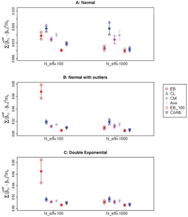
(A–C) Estimated mean and associated 95% confidence interval for the quantity ${({\widehat{\beta }}_{1,i}^{cor}-{\beta }_{1,i})}^2$, Where ${\widehat{\beta }}_{1,i}^{cor}$ is the corrected estimate for the log-OR for a particular SNP and β_1,i is the true underlying OR for the same SNP. The average was taken over genome-wide significant SNPs (having P < 0.05/10⁵) in 100 simulations of a given scenario—note that the number of selected SNPs for a given simulation, #{i: p_i < 0.05/10⁵}, is denoted as N_s in the y-axis label. Six methods were used to correct the log-ORs: Empircal Bayes (EB), Conditional Likelihood (CL), Conditional Mean (CM), the Average of CL and CM (Ave), the Empirical Bayes estimator using all 100 simulations to estimate the marginal distribution (EB_100), and the Combination estimator (Comb). The distribution of the true log-ORs were simulated according to a Contaminated Normal distribution (A), Double Exponential (B) or Normal Distribution (C). The number of nonzero log-ORs was either 100 or 1,000.

A few points are evident from these simulations as shown in Fig. 2A–C. First, for all three distributions, the Empirical Bayes method, EB in the figures, outperforms CM, CL, and Ave in the case where 1% of the SNPs are true signals, indicated by N_eff = 1,000 on the plots. However, in the cases where the number of effective SNPs is lower, the derivative of the log marginal density function becomes difficult to estimate because there are relatively fewer Z-scores in the tails, and as a result the density cannot be estimated as well. To emphasize that the deterioration in performance takes place as a result of misfitting the marginal distribution, we also display results from using all 100 simulations for a particular scenario to estimate the marginal distribution, before substituting the estimated marginal distribution into (7) (EB_100). In all six scenarios, EB_100 performs better than all other methods. Of course, the EB_100 estimator is unrealistic since in a real data situation one will not have the luxury of so many SNPs to estimate this marginal distribution. We include it here, just to emphasize that if the marginal distribution can be estimated well, the Empricial Bayes estimator will be optimal. In addition, comparing the three simulation distributions, it is worth noting that EB has the best relative performance when the log-ORs were generated from a normal distribution, since there are typically fewer extremely large log-ORs in this case compared to the simulations from the double exponential or contaminated normal; again, when there are some extremely large log-ORs and associated Z-scores, the tail of the marginal Z-scores distribution becomes more difficult to estimate and the performance of EB can break down. On a related note, we would expect the relative performance of EB to improve when the selection threshold is lowered, since again more information is available to estimate the marginal density function at lower values of Z. To emphasize this point, we examined the performance of all the shrinkage methods when a weak threshold of |Z| > 1.96 was used for selection of SNPs. (See Supporting Information Fig. S2 for more information.) In this case, the minimum observed mean square estimation error from the three Conditional Likelihood methods was a factor of between 4.28 and 129 times higher than the observed error for EB. As mentioned in “Methods” section, the combination estimator (denoted by Comb in Fig. 2) combines the strengths of the EB and the Conditional Likelihood estimators, by using one or the other depending on the length of the calculated confidence intervals. This strategy was very successful in reducing the overall squared error, and shows the best performance for the simulation models we considered.

In addition to the overall MSE, we estimate the MSE for specific Z-scores via loess regression (Supporting Information Fig. S3). To compare Empirical Bayes to Conditional Likelihood for a range of differing Z-values, it is necessary to choose different thresholds for significance when calculating the Conditional Likelihood estimator (here we choose thresholds of 1.96 and 5.02). The underlying message here is that the Empirical Bayes estimator is far more accurate for lower Z-scores (again where the marginal distribution is well estimated), but is outperformed by the Conditional Likelihood techniques for larger Z-scores in the tail of the marginal distribution. Again, the combination estimator is able to combine the best characteristics of both the estimators.

Finally, we examined the bias (measured by the average value of $\frac{1}{\#\{\text{significant}\}}{\sum }_{p_i<\frac{0.05}{{10}^6}}({\widehat{\beta }}_{1,i}^{cor}-{\beta }_{1,i})$ over the 100 simulation) for log-ORs, ${\widehat{\beta }}_{1,i}^{cor}$, corrected by each method, when the selection threshold of P < 0.05/10⁵ was used (see Supporting Information Fig. S4). At this threshold, Empirical Bayes tended to undershrink the estimated log-ORs, whereas the Conditional Likelihood approaches tended to overshrink. The combination estimator, which balances the Empirical Bayes and Conditional Likelihood estimators, was approximately unbiased.

Coverage of confidence intervals

We calculated 95% Bayesian confidence intervals using (9), with 100 bootstrap replications to estimate $\widehat{\mathrm{V}}\text{ar}(\frac{\mathrm{d}}{\mathrm{d}z}log\widehat{p}(z)$. The associated coverage probablity was compared to that obtained via Conditional Likelihood-based confidence intervals. The Bayesian intervals are not as well calibrated as the likelihood intervals; the coverage probability typically being between 90% and 95% (Table I). There are a number of possible reasons for the undercoverage. First, (9) is based on approximate normality of the posterior distribution given the particular Z-score and may not be accurate if this normality assumption fails. In addition, if there is bias in the estimator for log p(z), then $MSE(\frac{\mathrm{d}}{\mathrm{d}z}log\widehat{p}(z))>Var(\frac{\mathrm{d}}{\mathrm{d}z}log\widehat{p}(z)$ and subsequently (9) will have lower than 100(1 −α)% coverage. Finally, for computational feasiblity, the bootstrap estimator of $Var(\frac{\mathrm{d}}{\mathrm{d}z}log\widehat{p}(z)$ was calculated using a fixed number of degrees of freedom for the natural spline, whereas the actual estimate $\frac{\mathrm{d}}{\mathrm{d}z}log\widehat{p}(z))$ was derived via choosing the number of degrees of freedom using BIC. This may result in the estimated variance $\widehat{\mathrm{V}}\text{ar}(\frac{\mathrm{d}}{\mathrm{d}z}log\widehat{p}(z)$ being an underestimate of the true variability. It is possible that using bootstrap confidence intervals (as opposed to simply estimating the variance of $\frac{\mathrm{d}}{\mathrm{d}z}log\widehat{p}(z)$ by bootstrap and plugging the result into (9)), maybe better calibrated than the interval we consider here. However, such an approach would require more computational resources, since a larger number of bootstrap draws are required to estimate the endpoints of a confidence interval compared to generating a point estimate for a variance.

Analysis on Real Data

To compare the real data performance of Empirical Bayes shrinkage to the three Conditional Likelihood methods, we use an NIDDK Crohn's disease GWAS data set in which 1,082 Caucausian individuals were genotyped on 304,979 SNPs (after quality control). To replicate initial and follow-up cohorts, we randomly split the 1,082 individuals into two sets of 540 (270 cases and 270 controls) and 542 (274 cases and 268 controls) individuals.

We used logistic regression to estimate the log-ORs on the initial cohort for each SNP. Three different thresholds for selecting SNPs were compared, corresponding to P-value thresholds of 0.001,0.0001, and 0.00001. The Empirical Bayes method described above, the three Conditional Likelihood methods, and a recently proposed bootstrap approach [Sun et al., 2011] were then used to adjust the raw log-OR estimates for the selected SNPs. The average squared difference between the adjusted log-OR on the initial cohort for the selected SNPs and the estimated log-OR on the follow-up cohort for those same SNPs is used to measure the performance of each correction method. We plot this quantity (along with 95% confidence intervals) in Fig. 3A. The numbers of SNPs that pass each of the three significance thresholds is 252, 20, and 3, which explains the different widths of the associated confidence intervals. As a secondary real data example, we applied the same methods to correct the estimated log-ORs for a Schizophrenia data set downloaded from dbGaP (Study Accession: phs000017.v3.p1). Again we split the full data set (of 124,801 SNPs after standard quality control and Linkage Disequilibrium pruning) into training and test subsets (both having 578 cases and 689 controls), and examine the performance of each shrinkage method (given P-value thresholds of 0.001, 0.0001, and 0.00001) in the same way as before. Note that for both data sets, SNPs significantly associated at α = 0.00001—representing Z-scores above 4.41—are extremely rare—there being only 3 and 2 for the Crohn's disease and Schizophrenia data sets, respectively. Interestingly, the performance of the Empirical Bayes estimator does not break down even for these isolated SNPs. In both real data examples investigated, Empirical Bayes and the associated combination estimator have superior performance compared to the Conditional Likelihood and BR-squared methods at all three SNP-selection thresholds (see Fig. 3A and B).

Figure 3.

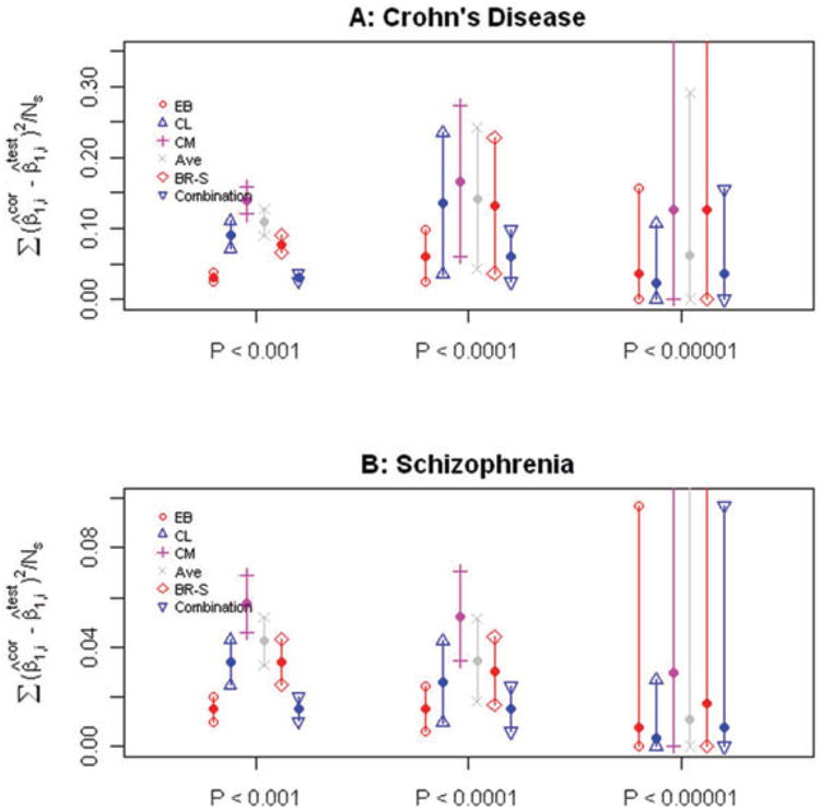
Performance on real GWAS data sets. (A–B) Estimated mean and associated 95% confidence interval for the quantity ${({\widehat{\beta }}_{1,i}^{cor}{-}_{{\beta }_{1,i}}^{\text{test}})}^2$, Where ${\widehat{\beta }}_{1,i}^{cor}$ is the corrected estimate for the log-OR for a particular SNP from the initial cohort and ${\widehat{\beta }}_{1,i}^{\text{test}}$ is the uncorrected OR estimate from the follow-up cohort. Five methods were used to correct the log-ORs: Empircal Bayes (EB), Conditional Likelihood (CL), Conditional Mean (CM), the average of CL and CM (Ave), BR-squared (BR-S), and the Combination estimator (Comb). The average was taken separately over the sets of SNPs meeting the significance thresholds (P < 0.001, P < 0.0001, P < 0.00001). The top panel represents Crohn's disease GWAS and the bottom panel Schizophrenia.

Discussion

In this article, we have proposed an alternative method to address the estimation bias related to the Winner's Curse. The approach we propose has a number of advantages over the Conditional Likelihood methods that are currently used. It has theoretical support in that it must be squared error optimal under the mixture model considered in section “Empirical Bayes estimation when f(μ) is unknown” if there is no error in estimating the marginal density for the standardized log-ORs. This implies that provided this marginal density can be estimated reasonably well in its tails, the proposed Empirical Bayes method should outperform Conditional Likelihood. In addition, we propose a modification of the estimator, by data-adaptively combining it with a previously studied Conditional Likelihood estimator, to ensure robustness of performance when the tails of this marginal distribution are difficult to estimate.

Comparing the proposed Empirical Bayes estimator to other common methods for correcting the Winner's Curse for two real GWAS data sets, the Empirical Bayes estimator recommends a more aggressive shrinkage of the raw log-ORs than does Conditional Likelihood or BR-squared, as shown in Supporting Information Fig. S5. In fact, we observe the best performance for the Empirical Bayes approach, even when shrinking the most highly associated SNPs as observed in Fig. 3. This is not the pattern we see in the simulated data sets, and it is probably unrealistic to expect this pattern for larger data sets or in different diseases (unless the true log marginal density function for the Z-scores is approximately linear in its tails as the natural spline would assume); here it may have more to do with the small sample sizes collected in both studies which restricts the possible magnitude of the actual Z-scores and results in a “nearly normal” marginal distribution that is easy to estimate. Nevertheless, even when if the distribution is poorly estimated in the tails, the combination estimator should still have excellent performance, as is observed in all scenarios for the simulation. On the other hand, we also have examined unpublished data (results not shown), and found a similar pattern—i.e., that the Empirical Bayes shrinkage method has better observed performance at all SNP-selection thresholds.

A nice feature of the proposed Empirical Bayes approach is that the correction applied to a given SNP, having a particular estimated log-OR and associated Z-score, will not change if the selection rule changes. In contrast for the Conditional Likelihood-based estimators, if it is decided to use an False Discovery Rate-based significance threshold, where before a Bonferoni threshold was used, the actual corrected log-ORs will change for all of the SNPs that were significant at the Bonferoni threshold, even though the data are exactly the same. In essence, the Empirical Bayes technique does not require the choice of a significance threshold for selection. While this property is lost for the combination estimator, it still holds approximately, in that the two estimators will disagree only on the subset of SNPs in the extreme tails of the distribution. The approach proposed is also very computationally convenient, allowing correction of hundreds of thousands of ORs in a matter of seconds on a personal computer. This distinguishes it somewhat from some more computational approaches such as the Boostrap approach proposed in Sun et al. [2011] and the spike and slab prior approach in Xu et al. [2011].

References

- Berger JO. Statistical Decision Theory and Bayesian Analysis Springer Series in Statistics. 2nd. New York: Springer; 1985. [Google Scholar]
- Capen EC, Clapp RV, Campbell WM. Competitive bidding in high-risk situations. J Pet Technol. 1971;23(6):641–653. [Google Scholar]
- Dudley RM. Real Analysis and Probability. Cambridge, UK: Cambridge University Press; 2002. [Google Scholar]
- Efron B. Empirical Bayes estimates for large-scale prediction problems. J Am Stat Assoc. 2009;104(487):1015–1028. doi: 10.1198/jasa.2009.tm08523. [DOI] [PMC free article] [PubMed] [Google Scholar]
- Efron B. Tweedie's formula and selection bias. J Am Stat Assoc. 2011;106(496):1602–1614. doi: 10.1198/jasa.2011.tm11181. [DOI] [PMC free article] [PubMed] [Google Scholar]
- Ghosh A, Zou A, Wright FA. Estimating odds ratios in genome scans: an approximate conditional likelihood approach. Am J Hum Genet. 2008;82(5):1064–1074. doi: 10.1016/j.ajhg.2008.03.002. [DOI] [PMC free article] [PubMed] [Google Scholar]
- Ogura Y, Bonen DK, Inohara N, Nicolae DL, Chen FF, Ramos R, Britton H, Moran T, Karaliuskas R, Duerr RH, Achkar JP, Brant SR, Bayless TM, Kirschner BS, Hanauer SB, Nuñez G, Cho JH. A frameshift mutation in NOD2 associated with susceptibility to Crohn's disease. Lett Nat. 2001;411:603–606. doi: 10.1038/35079114. [DOI] [PubMed] [Google Scholar]
- Sun L, Dimitromanolakis A, Faye LL, Paterson AD, Waggott D, Bull SB. BR-squared: a practical solution to the winners curse in genome-wide scans. Hum Genet. 2011;129(5):545–552. doi: 10.1007/s00439-011-0948-2. [DOI] [PMC free article] [PubMed] [Google Scholar]
- Wang WYS, Barratt BJ, Clayton DG, Todd JA. Genome-wide association studies: theoretical and practical concerns. Nat Rev Genet. 2005;6(2):109–118. doi: 10.1038/nrg1522. [DOI] [PubMed] [Google Scholar]
- Xiao R, Boehnke M. Quantifying and correcting for the winner's curse in genetic association studies. Genet Epidemiol. 2009;33(5):453–462. doi: 10.1002/gepi.20398. [DOI] [PMC free article] [PubMed] [Google Scholar]
- Xiao R, Boehnke M. Quantifying and correcting for the winner's curse in quantitative-trait association studies. Genet Epidemiol. 2011;35(3):133–138. doi: 10.1002/gepi.20551. [DOI] [PMC free article] [PubMed] [Google Scholar]
- Xu L, Craiu RV, Sun L. Bayesian methods to overcome the winners curse in genetic studies. Ann Appl Stat. 2011;5(1):201–231. [Google Scholar]
- Yang J, Benyamin B, McEvoy BP, Gordon S, Henders AK, Nyholt DR, Madden PA, Heath AC, Martin NG, Montgomery GW, Goddard ME, Visscher PM. Common SNPs explain a large proportion of the heritability for human height. Nat Genet. 2010;42:565–569. doi: 10.1038/ng.608. [DOI] [PMC free article] [PubMed] [Google Scholar]
- Yi N, Zhi D. Bayesian analysis of rare variants in genetic association studies. Genet Epidemiol. 2011;35(1):57–69. doi: 10.1002/gepi.20554. [DOI] [PMC free article] [PubMed] [Google Scholar]
- Zhong H, Prentice RL. Bias-reduced estimators and confidence intervals for odds ratios in genome-wide association studies. Biostatistics. 2008;9(4):621–634. doi: 10.1093/biostatistics/kxn001. [DOI] [PMC free article] [PubMed] [Google Scholar]
- Zhong H, Prentice RL. Correcting ‘winner's curse’ in Odds Ratios from genome wide association findings for major complex human diseases. Genet Epidemiol. 2010;34(1):78–91. doi: 10.1002/gepi.20437. [DOI] [PMC free article] [PubMed] [Google Scholar]
- Zollner S, Pritchard JK. Overcoming the winner's curse: estimating penetrance parameters from case-control data. Am J Hum Genet. 2007;80(4):605–615. doi: 10.1086/512821. [DOI] [PMC free article] [PubMed] [Google Scholar]
Associated Data
This section collects any data citations, data availability statements, or supplementary materials included in this article.