Site-Identification by Ligand Competitive Saturation (SILCS) Assisted Pharmacophore Modeling

Abstract

Database screening using receptor-based pharmacophores is a computer-aided drug design technique that uses the structure of the target molecule (i.e. protein) to identify novel ligands that may bind to the target. Typically receptor-based pharmacophore modeling methods only consider a single or limited number of receptor conformations and map out the favorable binding patterns in vacuum or with a limited representation of the aqueous solvent environment, such that they may suffer from neglect of protein flexibility and desolvation effects. Site-Identification by Ligand Competitive Saturation (SILCS) is an approach that takes into account these, as well as other, properties to determine 3-dimensional maps of the functional group-binding patterns on a target receptor (i.e. FragMaps). In this study, a method to use the FragMaps to automatically generate receptor-based pharmacophore models is presented. It converts the FragMaps into SILCS pharmacophore features including aromatic, aliphatic, hydrogen-bond donor and acceptor chemical functionalities. The method generates multiple pharmacophore hypotheses that are then quantitatively ranked using SILCS grid free energies. The pharmacophore model generation protocol is validated using three different protein targets, including using the resulting models in virtual screening. Improved performance and efficiency of the SILCS derived pharmacophore models as compared to published docking studies, as well as a recently developed receptor-based pharmacophore modeling method is shown, indicating the potential utility of the approach in rational drug design.

1. Introduction

Computational approaches are widely utilized nowadays to interact with experiments and expedite the process of drug discovery.[1,2] Once the disease related biological pathway and a potential target in that pathway, including the structure of the target, is known, structure-based drug design (SBDD) methods can be used to facilitate the drug design process. Based on the target structure, either force field based energetic descriptions of the target or interaction patterns of specific chemical types with the target can be explored and high-throughput virtual screening (VS) may be performed against a large chemical compound database to identify potential novel lead compounds. Typical SBDD methods include various docking techniques[3] and pharmacophore modeling methods.[4]

Docking techniques describe the target macromolecule and the test compounds using an energy function. The possible binding mode of a test compound is explored by minimizing its conformations in the potential field of the target, often “on-the-fly” during VS procedure. Representative docking methods include those implemented in the commonly used programs DOCK[5] and AutoDock.[6] Alternatively, pharmacophore modeling methods try to capture the crucial binding elements of compounds for a specific target in a more qualitative way. A three-dimensional (3D) pharmacophore model can be defined as spatially distributed chemical features that are essential for specific target-ligand binding. Such models contain both structural and chemical interaction information. As this represents a simplification of the detailed energetic information its efficiency is usually much higher than docking methods.

Receptor-based pharmacophore modeling techniques[7] usually use fragment based mapping methods[8] to explore all possible affinity features on a protein surface. This information is then used to elucidate the key features to create a pharmacophore model with which to perform VS. Representative receptor-based pharmacophore modeling methods include multi-copy simultaneous search (MCSS) derived pharmacophore methods,[9] GRID molecular interaction fields (MIFs) based methods[10] and the recent hydration-site-restricted pharmacophore (HSRP) method.[11]

Despite many successful applications of SBDD methods, a number of limitations are known. Most SBDD methods use only a single or limited number of target conformations and perform the docking or fragment mapping in vacuum or with an implicit solvent representation. Thus, the contributions of protein flexibility and aqueous solvation are subjected to significant approximations. The importance of including protein flexibility in VS is increasingly recognized[12,13] and inaccurate or even wrong answers may be obtained if VS is performed without inclusion of flexibility.[14,15] Aqueous environment also contributes to ligand binding[16] and its importance is emphasized by emerging methods that involve water molecule energetic analysis, such as WaterMap,[17] in computer-aided drug design (CADD).[18,19] Accordingly, methods that can address both issues to map the affinity pattern of a target are needed to improve the accuracy in VS.

Recently, the Site-Identification by Ligand Competitive Saturation (SILCS) method[20] was put forward to address these concerns. The SILCS method involves molecular dynamics (MD) simulations of the target protein immersed in an aqueous solution that contains additional organic solutes of different chemical classes. The solutes and water then compete for binding sites on the protein surface during the simulation, yielding a free energy fragment competition assay from which 3D fragment probability distributions of the solutes are used to define affinity patterns, termed FragMaps, encompassing a dynamic protein surface. SILCS FragMaps have been shown to correctly reproduce crystal binding modes of known ligand functional groups and, following conversion into Grid Free Energies (GFE), the SILCS method may be used to estimate relative experimental binding affinities.[21,22] Considering that the FragMaps define 3D distributions of favorable interaction regions distributed spatially on the protein surface, they can naturally be used as the basis for 3D pharmacophore features. Importantly, such FragMap based pharmacophore features will benefit from the explicit treatment of protein flexibility and solvation effect in the SILCS methodology.

In this study, we put forward a computational protocol that can generate receptor-based pharmacophore models using information from SILCS. This protocol includes conversion of SILCS FragMaps into pharmacophore features followed by pharmacophore hypotheses generation and ranking, with the resulting pharmacophores suitable for a range of VS screening tools. The protocol was validated using three representative protein targets along with ligands and decoys from the Dictionary of Useful Decoys (DUD).[23] Improved performance is seen for the SILCS-based pharmacophore model as compared to docking based VS using the common docking programs Dock and AutoDock and the recently developed receptor-based pharmacophore modeling technique of Lill and coworkers.[11]

2. Methodology and computational details

Overview of SILCS pharmacophore modeling procedure

Scheme 1 shows the overall procedure to generate SILCS pharmacophore models. The starting information for this protocol are the FragMaps obtained from SILCS simulations. FragMaps are fragment type 3D free energy maps generated on 1Ǻ×1Ǻ×1Ǻ cubic volume elements encompassing the entire simulation system, as previously described.[20] In the original SILCS setup, there are four types of FragMaps (aromatic, aliphatic, hydrogen-bond donor and acceptor) that are constructed from four fragment atom types (benzene carbons, propane carbons, water hydrogens and water oxygens, respectively). The FragMaps are normalized by the bulk voxel occupancies and probabilities are converted into GFEs based on a Boltzman distribution.[21] The voxels in these FragMaps are used as input for pharmacophore model development. Additional details of the SILCS methodology, FragMap generation and GFE calculations may be obtained from our previous publications.[20,21,24,25]

Scheme 1.

Workflow for generating SILCS pharmacophore models from SILCS FragMaps.

There are four key steps in the presented pharmacophore modeling protocol, described in detail below. The first step is to identify voxels that have favorable affinity within a pre-defined binding region on the target molecule. Next, these voxels are clustered to generate 3D FragMap features. The third step involves conversion of the FragMap features into SILCS pharmacophore features that can be used for VS. The final step combines the SILCS pharmacophore features into a collection of pharmacophore models (hypotheses), with those hypotheses being ranked based on GFE profiles as well as the number of pharmacophore features in each hypothesis. An in-house FORTRAN code, SILCS-Pharm, was written to automatically perform the whole protocol as well as convert the SILCS pharmacophore model into a format suitable for a number of VS packages.[26,27]

Voxel selection

GFE FragMaps define favorable binding patterns of the four chemical types that can be used to develop receptor-based pharmacophore features. The first step (Figure 1) of SILCS pharmacophore development is to identify all voxels that have GFEs lower than a user defined GFE cutoff value, thereby defining regions in which selected chemical types are critical for binding. Selection of the GFE cutoff must avoid the selection of too many features being located in the binding region (ie. GFE cutoff too high, or not favorable enough) as well as the selection of too few or no features in the binding regions (ie. GFE cutoff too low, or too favorable). Thus, the choice of the GFE cutoff should be made on a case by case basis, a decision that is facilitated by visualization of the FragMaps at different GFE cutoffs. However, based on previously studied protein systems, a GFE cutoff of −1.2 kcal/mol for aromatic/aliphatic FragMaps and −0.5 kcal/mol for water-based hydrogen-bond donor/acceptor FragMaps appear to be suitable for most systems, although different values were used in the present study (Table S1, supporting information). It should be noted that the suggested GFE cutoffs should not considered default values but initial guesses. Accordingly, it is highly recommended that the user determine appropriate cutoffs by visualizing the FragMaps for their specific case to determine at what GFE cutoffs well separated FragMap local regions of appropriate sizes (ideally single fragment size) are obtained that are suitable for the creation of the pharmacophore. Once the GFE cutoff levels for the different FragMaps are determined, the critical voxels on the protein surface required for the next step in pharmacophore development are selected.

Figure 1.

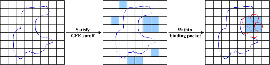
2D diagram of the first key step in pharmacophore model generation. The blue dotted shape represents a protein surface and each square corresponds to one voxel in the FragMaps. Blue colored squares represent voxels that have GFE values lower than the user input cutoff and red dotted circles or the rectangular region indicates the extent of the binding region to be considered for further pharmacophore development.

In principle further pharmacophore development could be performed on all the selected FragMap voxels on the entire target macromolecule. However, in practice a user defined binding region is used to focus pharmacophore development to regions of biological interest. The binding region may be selected based on experimental knowledge of, for example, the protein active site or the binding location of other inhibitors, with the extent of the region defined by a spherical or rectangular volume with the centroid and dimension information being provided. Alternatively, computational methods may be used to define the binding region, such as SPHGEN distributed with DOCK.[5] Examples of binding site boundary definitions are shown in Figure 1. In practice, subtle details of the definition of the binding region are not important as there are no FragMap voxels overlapping the protein itself and voxels at the edge of the defined region that are typically outside of the binding site such that they will be omitted during subsequent pharmacophore development due to their being excluded in the following clustering step.

Voxel clustering and generation of FragMap features

Individual voxels could be used to define pharmacophore features, though this would lead to a large number of small features. To overcome this, the FragMap voxels for the individual chemical types are clustered [10,11] into FragMap features. As the FragMap voxels of different types typically occupy well-separated volumes, connectivity based cluster algorithms, such as hierarchical clustering that builds clusters based on distance between objects,[28] are suitable for the present study (Figure 2). That is, all voxels within a distance cutoff, d, of each other will be put into one cluster and voxels from two different clusters will be separated by a distance greater than d.

Figure 2.

2D diagram of the second key step in pharmacophore model generation. Blue colored squares represent voxels satisfying the GFE cutoff in the binding pocket. Orange and green colored squares belong to voxel clusters identified by the hierarchical clustering algorithm using the cluster member distance parameter d. The GFE value for selected voxels is displayed. The orange and green circles are two FragMap features obtained from the two voxel clusters; their FGFE scores are also shown.

The distance cutoff, d, is the clustering algorithm parameter that can be assigned based on the following considerations. For the hydrogen bonding FragMaps, as there is only one oxygen atom in a water molecule and the distance between the oxygen and hydrogen atoms is less than the voxel edge length of 1 Ǻ, both hydrogen bonding donor and acceptor features can be captured by a single voxel or several neighboring voxels, and thus be in the same cluster. The minimum distance between two voxels refers to the smallest distance that can be found between two points within the two voxels. Accordingly, as the voxel size is 1Ǻ×1Ǻ×1Ǻ, a distance cutoff of 1 Ǻ for clustering of voxels for hydrogen-bond donor and acceptor type will lead to all voxels connected to each other contributing to the same cluster. However, for aromatic and aliphatic type voxels, where carbon atoms are used, a distance cutoff of 2.8 or 2.6 Ǻ is used as they correspond to the distance between the two most separated carbon atoms in a single benzene or propane molecule, respectively. In principle, such distance cutoffs are long enough to ensure that all voxels associated with one benzene or propane fragment will be included in the same cluster.

From the voxel clusters for the four FragMaps, FragMap features are defined to facilitate their use in the context of a pharmacophore. FragMap features are defined as a sphere with the center being the geometric center of the voxel cluster. An alternative that was considered was the GFE weighted geometric center; in practice this was very similar to the simple geometric center and, thus, was not used. The sphere radius is subsequently calculated such that the sphere will include all the voxels in a cluster (Figure 2).

FragMap features may also be assigned energies based on the GFE score of the voxels defining each FragMap feature. These energies, termed the feature GFE (FGFE), are defined as the sum of all voxel GFEs of the n voxels contained in a cluster as shown in equation 1.

$$FGF{E}_j=\sum _{i=1}^{n}GF{E}_{ith\_\mathit{\text{voxel}}\_\mathit{\text{in}}\_jth\_\mathit{\text{cluster}}}$$ (1)

Other options to define the FGFE that were considered, including the cluster member number weighted GFE which may represent the GFE efficiency of that voxel cluster. However, considering that each voxel cluster ultimately represents the binding mode of a single chemical entity, larger voxel clusters likely represent entities that make a larger contribution to binding, though it should be noted smaller clusters comprised of voxels with very favorable GFE scores may also make large contributions to binding. Accordingly, the simple summation in equation 1 was selected to assign energies to the FragMap features. Examples of FragMap features are shown diagrammatically in Figure 2.

Convert FragMap features to SILCS pharmacophore features

For their use with various pharmacophore VS programs, the FragMap features need to be converted to “SILCS pharmacophore features.” There are two main differences between FragMap features and SILCS pharmacophore features. First, in addition to the four basic FragMap feature types, there are joint features where more than one FragMap feature type is located at a specific position. For example, a spatial region on the protein surface that can encompasses both aromatic or aliphatic FragMap features can be assigned a joint aromatic-aliphatic feature. Second, the FragMap hydrogen-bond donor feature is defined by the water hydrogen atoms, but hydrogen-bond donor pharmacophore features usually use the parent heavy atom instead of hydrogen atom to define such features.

To address the first concern, aromatic-aliphatic and hydrogen-bond donor-acceptor joint features are considered separately. To generate aromatic-aliphatic joint features, the overlap between each individual aromatic and aliphatic FragMap feature is analyzed. The extent of overlap that enables creation of a joint feature is defined as more than half of the volume of one FragMap feature being overlapped by a second feature as defined in equation 2,

$$d_{\mathit{\text{Arom}}-\mathit{\text{Alip}}}=C_{\mathit{\text{Arom}}}-C_{\mathit{\text{Alip}}}\le R_{\mathit{\text{Arom}}}|R_{\mathit{\text{Alip}}}$$ (2)

where d is the distance between two FragMap feature centers, C is the feature center and R is the feature sphere radii as shown in Figure 3. For example, effective overlap is found in cases 2 (d_Arom−Alip < R_Alip), 3 (d_Arom−Alip < R_Arom) and 4 as shown in Figure 3 while case 1 (d_Arom−Alip > R_Arom & R_Alip) does not have a sufficient overlap. If there is an effective overlap, one joint SILCS pharmacophore feature is created with the sphere center being set to the geometric center of the volume occupied by the two or more original FragMap features with the sphere radius being set to let the joint SILCS pharmacophore feature encompass the two or more original FragMap features. The FGFE score for the joint SILCS pharmacophore features, FGFE_Arom|Alip, is the sum of the FragMap feature FGFEs, consistent with the additive nature of voxel occupancy that is used to calculate voxel GFEs. For example, consider a case where one benzene and one propane resides at the same location for half of the SILCS simulation time, the corresponding FGFE_Arom and FGFE_Alip values would be 50% of that if one type occupied that location. Thus, the joint SILCS pharmacophore feature would involve occupation of the site 100% of the simulation time, approximately equivalent to the sum of FGFE_Arom and FGFE_Alip. Thus, all hydrophobic FragMap features are either aromatic or aliphatic SILCS pharmacophore features or combined aromatic-aliphatic joint SILCS pharmacophore features (Figure 3).

Figure 3.

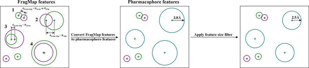
2D diagram illustrating how the hydrophobic SILCS pharmacophore features are generated based on aromatic (purple circles) and aliphatic (green circles) FragMap features in the third key step of generating pharmacophore models from FragMaps. The joint Arom|Alip pharmacophore features are colored by cyan. Feature sphere centers are shown by plus sign in corresponding colors.

Hydrogen-bond FragMap features need additional consideration when being converted into SILCS pharmacophore features. As water is used to represent both hydrogen-bond donor and acceptor functionalities during the SILCS simulation, it is difficult to differentiate between specific waters that served as a donor or acceptor or both based on the FragMaps alone. This can be overcome using protein surface information together with hydrogen-bond FragMap features. In this approach, the protein surface is generated using the DMS tool distributed with the Chimera software package[29] based on the average protein structure over all of the SILCS trajectories. The protein surface point closest to a FragMap feature is chosen as a reference point for this feature. When there is no overlap between a FragMap acceptor feature and any hydrogen-bond donor FragMap features, the hydrogen-bond acceptor FragMap feature is directly defined as a hydrogen-bond acceptor SILCS pharmacophore feature. For donor FragMap features with no overlap, a new sphere is created, as shown in Figure 4(a), to represent the related heavy atom location and is used as a hydrogen-bond donor SILCS pharmacophore feature. The new sphere is generated with the outer most point on the new sphere 1.05 Ǻ away from the original sphere in the direction defined by a vector pointing from the protein surface reference point to the original sphere. The sphere center and radius for the new FragMap feature is calculated accordingly. Essentially, the surface reference point represents the location of a protein hydrogen-bond acceptor participating in hydrogen-bond interactions with the hydrogen-bond donor FragMap feature, which now represents a hydrogen-bond donor SILCS pharmacophore feature with both distance and angular considerations. The 1.05 Ǻ distance is the average hydrogen-heavy atom covalent bond length considering both hydroxyl and amide groups. The larger radius of the new sphere accommodates a wide range of hydrogen-bond angles (three D-H…A hydrogen-bond interaction cases as shown on the right of Figure 4(a)). Preliminary results showed this approximation to work satisfactorily and thus can serve as a very efficient way to convert a hydrogen-bond donor FragMap features into a SILCS pharmacophore feature.

Figure 4.

2D diagram illustrating generation of the hydrogen-bond SILCS pharmacophore features based on hydrogen-bond donor (blue solid line circles) and acceptor (red circles) FragMap features in the third key step of pharmacophore model generation. The joint Hdon&Hacc pharmacophore features are pink spheres. Feature sphere centers are shown by a plus sign in the corresponding colors. Symbols A and D represent hydrogen-bond acceptor and donor heavy atom, respectively. (a) Determination of hydrogen-bond donor pharmacophore features (parent heavy atom of hydrogen, blue dashed line circles) from hydrogen-bond donor FragMap feature sphere (hydrogen, blue solid line circles). (b)–(g) Generation of pharmacophore features when one overlap is found between one hydrogen-bond donor and one acceptor FragMap feature.

When there is an overlap between a hydrogen-bond donor and an acceptor FragMap feature, the final SILCS pharmacophore feature is determined based on the effective overlap between the hydrogen-bond FragMap features as follows:

$$d_{\mathit{\text{Hdon}}-\mathit{\text{Hacc}}}=C_{\mathit{\text{Hdon}}}-C_{\mathit{\text{Hacc}}}\le (R_{\mathit{\text{Hdon}}}+1.05)|(R_{\mathit{\text{Hacc}}}+1.05)$$ (3)

The value of 1.05 Ǻ again accounts for the covalent bond to the heavy atom. Similar to the hydrophobic case, d_Hdon−Hacc is the distance between the two sphere centers C_Hdon and C_Hacc. If this distance is equal or smaller than the sum of the radii of either donor or acceptor spheres plus 1.05 Ǻ the features are considered overlapping. Four cases are possible when overlapping hydrogen-bond donor and acceptor FragMap features are identified as shown in Figures 4(b) to 4(g). Two distance cutoffs, 0.9 Ǻ for hydrogen-bond donor FragMap features and 1.2 Ǻ for acceptor FragMap features demarcate the first two cases. They determine if the FragMap features form direct interactions with the protein or are only present due to its associated acceptor or donor FragMap feature forming a direct hydrogen bond with the protein. The value of 0.9 Ǻ is calculated as 2.4 Ǻ minus 1.5 Ǻ, where 2.4 Ǻ is the average donor hydrogen atom to acceptor heavy atom distance for a common hydrogen bonds,[30] and 1.5 Ǻ is the average radius used by DMS when generating protein surface around nitrogen and oxygen atoms. Similarly, 1.2 Ǻ is calculated as 2.4 Ǻ minus 1.2 Ǻ, where 1.2 Ǻ is used by DMS for hydrogen atoms to generate the protein surface. When the distance between the donor feature and its protein surface reference point (d_Hdon−Surf) is less than 0.9 Ǻ while the distance between the acceptor FragMap feature and its reference point (d_Hacc−Surf) is larger than 1.2 Ǻ (Figure 4(b)) the hydrogen-bond donor interacts with the protein directly, such that the FragMap features are combined into one hydrogen-bond donor SILCS pharmacophore feature. In this case, the acceptor sphere naturally defines the location of heavy atom associated with the donor sphere, thus the geometry of the acceptor FragMap feature and the FGFE score of the donor FragMap feature sphere are assigned to this new donor SILCS pharmacophore feature. Similarly, when d_Hdon−Surf is larger than 0.9 Ǻ and d_Hacc−Surf is less than 1.2 Ǻ (Figure 4(c)), then the hydrogen-bond acceptor FragMap feature is defined as a hydrogen-bond acceptor SILCS pharmacophore feature.

When both the donor and acceptor FragMap features satisfy their distance cutoffs then a single water molecule serves as both hydrogen-bond donor and acceptor and forms dual hydrogen-bond interaction with the protein. Two possible SILCS pharmacophore features may be generated in this case (Figure 4(d)–4(g)). To differentiate between these two cases, the associated feature as defined in Figure 4(a) is first generated for the hydrogen-bond donor FragMap feature. Then, if there is no overlap with the acceptor feature and there is also no clash between the donor associated feature and the protein surface, as shown in Figure 4(d), then the two formally overlapping FragMap features are treated separately and converted into two SILCS pharmacophore features. This scenario corresponds to a situation that mimics a hydroxyl or two adjacent functional groups acting as a donor and a acceptor (Figure 4(e)). In the final scenario, when a hydrogen-bond donor FragMap feature sphere overlaps with an acceptor feature (Figure 4(f)) or clashes with the protein surface (Figure 4(g)), indicating either the lack of need or space for additional hydrogen-bond groups in the local region, then the hydrogen-bond donor and acceptor FragMap features are combined into one joint SILCS pharmacophore feature (Hdon&Hacc). The geometry is based on the acceptor sphere and the FGFE_Hdon&Hacc score is the sum of the original FGFE scores.

Finally, a size filter is applied to refine the generated SILCS pharmacophore features. Currently, the radii of the features are capped at 2.5 Ǻ for hydrophobic features and 1.5 Ǻ for hydrogen-bond features (Figure 3). This in done to prevent features having large radii caused by high GFE cutoffs being used when initially selecting voxels for feature development (Figure 1).

SILCS Pharmacophore Model Generation

The SILCS pharmacophore features from the previous step are next used to generate all possible pharmacophore hypotheses. By default, only hypotheses with more than two features are considered. All generated hypotheses are then sorted based on the number of features and all the hypotheses with the same number of features ranked with a hypothesis GFE (HGFE) score, which is defined as the sum of FGFEs of the individual SILCS pharmacophore features in a hypothesis.

$$HGF{E}_j=\sum _{i=1}^{n}FGF{E}_{ith\_\mathit{\text{feature}}\_\mathit{\text{in}}\_jth\_\mathit{\text{hypothesis}}}$$ (4)

The user may then visualize selected hypothesis to understand their spatial relationship with respect to the targeted binding site, with respect to known ligands and so on to select the final SILCS pharmacophore model for VS. Usually, hypotheses with up to 6 features are used for VS as a hypothesis with more features will significantly limit potential candidates. In the current study, the SILCS pharmacophore models are created in MOE format, allowing for their use in pharmacophore VS using MOE.[26] Models may also be readily generated in formats suitable for a wide selection of VS software packages.

Testing data set and SILCS FragMaps

SILCS pharmacophore model validation used the DUD database.[23] The DUD database is a widely employed benchmark data set for VS methods as it provides very challenging decoys for each ligand of a target along with known ligands of the target protein. The decoys in DUD resemble known ligands with respect to physical properties and thus avoid bias caused by weak decoys that are very dissimilar to known ligands and, thus, may be easily distinguished by VS methods. The protein targets used in this study include HIV protease (HIVPR), Factor Xa (FXa) and dihydrofolate reductase (DHFR). These proteins come from different protein families (serine proteases, folate enzymes and other enzymes according to the classification in Ref [23]) and their DUD ligand and decoy data sets having different sizes (number of unique ligands and decoys range from 53 to 201 and 1885 to 7145, respectively (Table 1)). In addition, they have been used in published VS studies,[11] allowing for comparison with those studies.

SILCS simulations for protein targets HIVPR and FXa have been performed previously[21] and the associated FragMaps were used here as inputs for pharmacophore modeling. For DHFR, SILCS simulations were performed using the published setup and are summarized briefly. The structure of DHFR was extracted from the crystal holo structure in the Protein Data Bank (PDB)[31] (PDB ID: 3DFR[32]) that was also used in DUD database development.[23] The ligand and the nicotinamide adenine dinucleotide phosphate coenzyme were removed and crystal waters were retained. System preparation used the Reduce software[33] and the SILCS simulations were performed with CHARMM[34] and the CHARMM22 protein force field[35] with CMAP[36] and the TIP3P water model.[37] Remaining methodological details were as published[20,21] with the FragMaps obtained from the final 5 ns of ten 20 ns MD simulations. Results from the SILCS simulations are presented in Figure S1 and discussed in the supporting information.

Pharmacophore model VS and performance evaluation

The MOE software package[26] was used here to perform VS. All ligands or decoys for a target, initially in mol2 formatted files, were converted into MOE compound database mdb formatted files and then used to generate ligand conformations using the “Conformation Import” application in MOE.[26] Up to 100 low-energy conformations defined by the MMFF94x force field[38] were generated for each molecule using default MOE settings. SILCS pharmacophore models in MOE pharmacophore search query file format were used in conjunction with the ligand conformational databases with default settings. Pharmacophore VS was performed in full matching mode such that all features in the pharmacophore model need to be matched for a compound to pass the VS. The pharmacophore search engine in MOE first annotates each ligand with pharmacophore features and then attempts to match these features with the pharmacophore model by repositioning each ligand conformation to minimize the root-mean-square deviation (RMSD) between the matched features in the molecule and the query pharmacophore model. The RMSD of the best matched conformation for each molecule was then used as a theoretical activity score.

To compare the performance of SILCS pharmacophore modeling with other VS methods, docking based VS was carried out using two common docking packages DOCK 4.0[5] and AutoDock4.[6] Version 4.0 of DOCK, which includes in house modifications, was used, with the sphere set files used to define the binding sites also used to prepare scoring grids and initialize the docking procedure. An in-house DOCK protocol, which adopts approaches applied in a number of in-house CADD projects. [39,40] was used in the context of the anchor-based build up procedure[5] with the final ligand conformations selected based on the most favorable interaction energy calculated as the sum of electrostatic and van de Waals (vdW) energies with that score used for final energy score ranking. For docking studies using AutoDock, mol2 formatted files from DUD were first converted to pdbqt formatted files to generate AutoDock atom types.[6] The binding site for each target was defined in the same way as for DOCK and the protein structures used by DUD were used to generate energy grid map files with probe atoms covering all possible molecule atom types within the database. Conformational searching with AutoDock was guided by the Lamarckain genetic algorithm (LGA)[41] and 20 independent runs with a maximum of 1750000 energy evaluations and 27000 GA generations were performed. The energy score used in AutoDock includes electrostatic, vdW and desolvation terms.[41] Energy scores of the 20 conformations for each molecule were averaged and the mean value was used for the final energy score ranking.

To evaluate VS performance, enrichment plots, as used in the DUD development,[23] showing the percentage of ranked ligands at any given percentage of ranked database were employed. In order to compare our results directly with another pharmacophore modeling study using DUD,[11] the Receiver Operating Characteristic (ROC) curve,[42] showing the percentage of ranked ligands at any given percentage of ranked decoys, was also plotted. Enrichment factor (EF) reflecting the ability of a method to find more true positives while maintain a low level of false positive rate is calculated following ranking of all the ligands and decoys, as follows:

$$E{F}_{\mathit{\text{subset}}}=\frac{N_{\mathit{\text{ligands}}\_\mathit{\text{in}}\_\mathit{\text{subset}}}/N_{\mathit{\text{ligands}}}}{N_{\mathit{\text{decoys}}\_\mathit{\text{in}}\_\mathit{\text{subset}}}/N_{\mathit{\text{decoys}}}}$$ (5)

where subset is defined by the percentage of the ranked decoys, N_{ligands_in_subset}, N_ligands, N_{decoys_in_subset} and N_decoys are the number of ligands in a subset, total number of known ligands, number of decoys in a subset and total number of decoys. EFs at 1% (EF₁), 10% (EF₁₀) and 20% (EF₂₀) of the ranked decoys represent early and later stage enrichment performance. The area-under-the-curve (AUC) was also evaluated from the ROC plot to assess the quality of enrichment.

In contrast to docking based VS, which can always pose a molecule in the binding pocket, a pharmacophore hypothesis serves as a filter for molecules in the database such that some molecules with insufficient features matching the pharmacophore will not pass the VS and thus no score will be assigned. To allow for direct comparison of the docking and pharmacophore VS methods, failed ligands and decoys are ranked at the end of the ranking list with decoys ranked above ligands (e.g. with 4 unranked decoys (D) and 2 unranked ligands (L) they would be assigned the order of DDLDDL).

3. Result and discussion

Generation of SILCS assisted pharmacophore models

FragMaps for HIVPR and FXa were obtained from a previous study[21] with FragMaps for DHFR generated as part of the present study (see the supporting information and Figure S1 for details). It should be noted that the quality of a SILCS pharmacophore model fully depends on the quality of FragMaps. As described previously[21] and in the current supporting information, the FragMaps do capture the important interaction patterns of the tested protein targets. Accordingly, it can be expected that the SILCS pharmacophore models will be consistent with known interaction patterns of the studied protein targets.

Pharmacophore models were generated using the SILCS-Pharm code as described above. To be consistent with DUD and make fair comparison with the other docking methods that use DUD default parameters, DUD setup files were used as much as possible to initialize the pharmacophore generation with the sphere set files used to define the location and shape of the binding sites adjusted here to serve as the input to SILCS-Pharm. The adjustment is required due to the previous sphere sets being based on rigid receptor structures while the SILCS FragMaps integrate the flexibilities of the targets and thus the size of some spheres had to be increased to accommodate all the occupied SILCS voxels. The GFE cutoffs used for the hydrogen-bond donor and acceptor FragMaps were adjusted in a way that the final hydrogen-bond donor and acceptor FragMap features have only one or zero overlaps, i.e. only the crucial water binding modes are retained. GFE cutoffs for the hydrophobic FragMaps were also adjusted to maintain a limited number of aromatic and aliphatic binding patterns in the pocket. GFE cutoffs used for the three targets are listed in Table S1 in the supporting information.

Validation of the SILCS pharmacophore model development methodology

Before using SILCS pharmacophore models for VS, the suggested methodology used to generate the pharmacophore models requires validation. Four aspects need to be addressed: 1) if the identified voxel clusters and subsequent FragMaps features encompass the favorable binding patterns as indicated by FragMaps; 2) if the hydrophobic SILCS pharmacophore features are being generated appropriately from FragMap features; 3) if the hydrogen-bonding SILCS pharmacophore features are being generated appropriately from FragMap features; and 4) if the HGFE score is a suitable index to rank pharmacophore hypotheses for use in VS. To validate these four aspects, the various components of the pharmacophore models were generated for the three testing targets and compared visually with FragMaps.

To address the first concern, aliphatic voxels below the GFE cutoffs used to generate the FragMap aliphatic features and related FragMap feature spheres are shown in Figure 5 together with aliphatic FragMaps. For all the three test cases the identified voxel clusters (orange dots) and related FragMap features (transparent green spheres) can efficiently cover the local FragMap regions (green wireframes). It should be noted that some FragMap features penetrate into the crystal structure surface as the SILCS method explicitly incorporates protein flexibility into the FragMaps. Other types of voxel clusters and related FragMap feature spheres were also checked and comparisons with the corresponding FragMaps to further verify that the current clustering algorithm used in the pharmacophore development can efficiently resemble the binding patterns present in FragMaps.

Figure 5.

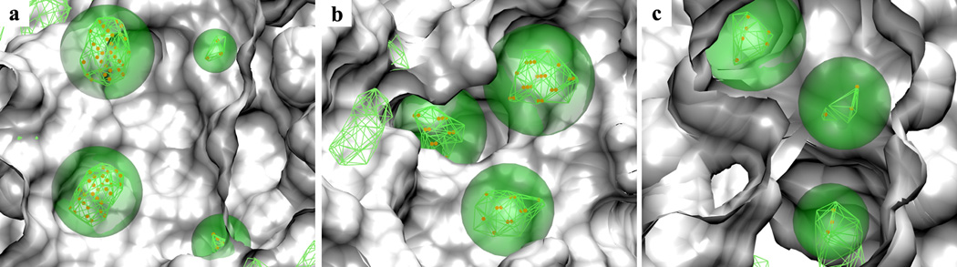
Aliphatic FragMap features (green transparent spheres) generated from aliphatic FragMaps (green wireframes) based on voxel clustering (orange dots). The FragMaps are presented at GFE cutoffs that were used to generate the pharmacophore models. The surfaces of the crystal protein structures used to initialize SILCS simulations are shown for the three protein targets (a) HIVPR (PDB ID:1G2K), (b) FXa (PDB ID:1MQ5) and (c) DHFR (PDB ID:3DFR). Regions of the protein occluding the view are removed from the visualization.

To verify the ability of the method to convert hydrophobic FragMap features into SILCS pharmacophore features, all hydrophobic features were checked for the three targets. Figure 6 shows the obtained hydrophobic SILCS pharmacophore features together with aromatic and aliphatic FragMaps at the GFE cutoffs that were used to develop the pharmacophore features. Based on knowledge of key interaction patterns in the binding pockets for HIVPR,[21,43] FXa[44,45] and DHFR,[32,46] all hydrophobic binding regions in the designated binding pockets can accommodate both aromatic and aliphatic chemical groups. And consistent with this, the generated SILCS pharmacophore features are all of the Arom|Alip type for all three targets. In addition, for all three test cases, the SILCS pharmacophore features cover both the aromatic and aliphatic FragMaps quite well, verifying the reliability of the method to determine the geometry of the joint hydrophobic SILCS pharmacophores. For example, the position of the bottom right Arom|Alip pharmacophore feature shown in Figure 6(a) covers both the aromatic and aliphatic FragMap features in that region. In another example, the two aliphatic FragMap features shown at the top of Figure 5(c) were combined into one single Arom|Alip pharmacophore feature sphere as shown at the top of Figure 6(c) associated with their effective overlap with the aromatic FragMap feature sphere between them as indicated by the aromatic FragMap region shown at the top of Figure 6(c). Thus, the present approach allows for simplification of FragMap features into a small number of SILCS pharmacophore features that sufficiently model the functional group requirements of the targets.

Figure 6.

Hydrophobic SILCS pharmacophore features (joint Arom|Alip feature spheres in cyan color) generated from aromatic (purple wireframes) and aliphatic (green wireframes) FragMaps associated hydrophobic FragMap features for the three protein targets (a) HIVPR (PDB ID:1G2K), (b) FXa (PDB ID:1MQ5) and (c) DHFR (PDB ID:3DFR). Regions of the protein occluding the view are removed from the visualization.

It should be noted that some FragMaps in Figure 6 are not being fully covered by the SILCS pharmacophore features due to the pre-defined size filter. The filter was used to avoid possible bias caused by using a less unfavorable GFE cutoff resulting in a large region being included in the feature development and thus make the pharmacophore feature nonspecific. However, despite the cutoff, all important FragMap regions are covered effectively by the generated SILCS pharmacophore features.

Unlike the well-defined hydrophobic features, the hydrogen-bond pharmacophore features are determined based on a number of assumptions. Verification of the current protocol’s ability to generate hydrogen-bond pharmacophore features includes checking if the proposed protocol can predict the position of the hydrogen-bond donor parent atom correctly and if the overlapping FragMap features can be treated appropriately to generate single or joint pharmacophore features. Figure 7 shows the SILCS hydrogen-bond pharmacophore features for the three targets together with the hydrogen-bond donor and acceptor FragMaps. To judge if the positions of the pharmacophore features have been generated correctly, nearby protein residues that have key hydrogen-bond interactions with possible ligand functional counterparts are also shown. For HIVPR, one hydrogen-bond donor and one acceptor SILCS pharmacophore feature were generated which is consistent with the two known hydrogen-bond key interactions for HIVPR ligands at the flap site and catalytic site on the protein surface.[21,43] For the hydrogen-bond acceptor pharmacophore feature, the center (orange dot) of the generated feature sphere (red transparent sphere) sits at the geometric center of the hydrogen-bond acceptor FragMap region (red wireframe) near the backbone amides of Ile50 of both protein monomers. For the hydrogen-bond donor sphere, the center of the generated FragMap feature (blue transparent sphere) is slightly shifted from the hydrogen-bond donor FragMap region in the direction pointing from the Asp25 side chains to the FragMap region. As there are two Asp25 residues from the protein dimer, the FragMap feature is found between the two residues. For FXa, hydrogen-bond donor and acceptor pharmacophore features were generated which correspond with potential hydrogen-bond interaction with residues Asp189 and Ser195. The center of the hydrogen-bond acceptor sphere overlaps with the hydrogen-bond acceptor FragMap region near residue Ser195. The hydrogen-bond donor feature sphere is away from the center of the donor FragMap region in the direction opposite to Asp189. Similar relationships are observed for DHFR where three hydrogen-bond donor feature spheres were generated.

Figure 7.

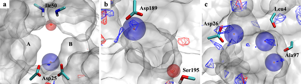
Hydrogen-bond donor (blue spheres with orange dot showing the sphere center) and acceptor (red spheres) SILCS pharmacophore features generated from hydrogen-bond donor (blue) and acceptor (red) FragMaps for the three protein targets (a) HIVPR (PDB ID:1G2K), (b) FXa (PDB ID:1MQ5) and (c) DHFR (PDB ID:3DFR). Regions of the protein occluding the view are removed from the visualization.

The geometries of the generated hydrogen-bond features are reasonable considering their spatial relationship with corresponding protein residues with which they may form hydrogen bonds. This verifies that the protocol used to generate hydrogen-bond SILCS pharmacophore features is able to identify the correct heavy atom positions related to the corresponding hydrogen-bond donor or acceptor FragMaps. Similar to that for hydrophobic features, the protocol also has the ability to effectively simplify the FragMap features and generate less but essential SILCS pharmacophore features. For example, considering DHFR, the generated hydrogen-bond donor feature shown at the left of Figure 7(c) encompasses three localized donor FragMap regions near residue Asp26, which represent three individual hydrogen-bond donor FragMap features.

Using the current GFE cutoffs to generate pharmacophore features for the three targets did not create joint hydrogen-bond pharmacophore features. To test the ability of the protocol to determine joint hydrogen-bond features, the hydrogen-bond GFE cutoffs for FragMaps of HIVPR were raised to increase the overlap between localized donor and acceptor FragMap regions. This results in two Hdon&Hacc joint SILCS pharmacophore features as shown in Figure 8. The Hdon&Hacc joint features nicely overlap with donor and acceptor FragMaps adjacent to Asp29 in HIVPR monomer A (Figure 8(a)) and Asp30 in monomer B (Figure 8(b)). In both cases the protein functional groups serve as both hydrogen-bond acceptor and donor corresponding to the donor and acceptor FragMaps. These further analyses verify the ability of the protocol to determine joint hydrogen-bond pharmacophore features.

Figure 8.

Hdon&Hacc joint SILCS pharmacophore features (pink sphere with orange dot showing the sphere center) generated from hydrogen-bond donor (blue) and acceptor (red) FragMaps for protein target HIVPR (PDB ID:1G2K). Regions of the protein occluding the view are removed from the visualization.

Finally, the ability of the FGFE scores to predict the priority of features and related HGFE used as a ranking score for SILCS pharmacophore hypotheses is examined. The hypotheses with 6, 4 and 4 SILCS pharmacophore features with the lowest HGFE among all generated hypotheses with the same number of features for HIVPR, FXa and DHFR, respectively, are presented in Figure 9. The crystal structure of a representative ligand for each target is also shown in the figure. It can be seen that the best hypothesis for all the targets contain features that correspond to well-known key interaction patterns for ligands with their respective targets. This is evident by the good overlap of the SILCS pharmacophore features with functional groups of the same chemical type in the ligands. For example, for HIVPR (Figure 9(a)) the overlaps of the four Arom|Alip features with the four aromatic groups in the ligand are seen as well as overlaps of the hydrogen-bond acceptor feature with carbonyl oxygens and overlap of the hydrogen-bond donor feature with likely hydrogen positions in the hydroxyl groups in the ligand.

Figure 9.

The best HGFE scored SILCS pharmacophore hypotheses with 6, 4 and 4 features, respectively, for (a) HIVPR, (b) FXa and (c) DHFR. Hydrophobic Arom|Alip, hydrogen-bond donor and acceptor features are shown by cyan, blue and red color wireframe spheres. Representative crystal structures for the protein and ligand are overlaid with the hypotheses for (a) HIVPR (PDB ID:1QBS), (b) FXa (PDB ID:1XKB) and (c) DHFR (PDB ID:3DFR). Regions of the protein occluding the view are removed from the visualization.

The power of the HGFE used to rank hypotheses is more evident if several top ranked hypotheses are examined. For example, for target DHFR, as shown in Figure 6(c) and 7(c), there are two hydrophobic and three donor SILCS pharmacophore features in the binding site. Thus there are five different hypotheses containing four features. The top three HGFE ranked hypotheses all have the two hydrophobic features together with other two hydrogen-bond donor features. This is consistent with the known importance of two hydrophobic features being important for the binding of DHFR ligands.[32,46] Besides the two hydrophobic features, the best hypothesis as shown in Figure 9(c) has the third and forth features that are known to form important hydrogen-bond interactions with DHFR by the two amine groups present in the pyrazine ring of MTX.[46] Similar observations can be found for FXa where one donor and one acceptor pharmacophore feature was derived from the SILCS FragMaps in addition to the three hydrophobic features. For the generated 4-feature hypotheses, the two top-ranked hypotheses have the three hydrophobic features that are known to be very important for the binding of FXa ligands.[44,45] The best hypothesis as shown in Figure 9(b) has the fourth feature as a hydrogen-bond donor instead of the acceptor feature, which is consistent with findings that hydrogen-bond donors are conserved among FXa ligands associated with interactions with Asp189.[45] The three test cases support that the use of HGFE scores are appropriate for ranking of SILCS pharmacophore hypotheses.

SILCS based pharmacophore VS

VS was performed using the selected SILCS pharmacophore hypotheses based on the most favorable HGFE scores. For HIVPR, hypotheses with 4, 5 and 6 features were tested while for FXa and DHFR hypotheses with 3 and 4 features were tested. Performance of the presented method was compared against two VS docking methods using Dock and Autodock and against recently presented pharmacophore models[11] that include consideration of solvation effects and targeted the same test systems.

The success of a pharmacophore VS not only depends on the pharmacophore features but also on the sampled conformations of the compounds. As the current study is not focused on identifying the most appropriate pharmacophore VS protocol for a specific target but just as a proof-of-concept study, the ligand conformations were generated using MOE with default MMFF94x force field and only 100 low-energy conformations were prepared. Either increasing the number of conformations or using a different force field for conformational sampling may impact the VS results.

Figure 10 shows the VS enrichment plots using the SILCS pharmacophore models for the three targets as well as docking results using DOCK and AutoDock. The random control line, which represents the result obtained when selecting ligands randomly (ligands and decoys are ranked evenly), is also shown. ROC plots, which give a similar picture as the VS enrichment plots, are shown in Figure S2 in the supporting information. For all three test cases, enhanced enrichment was found when using SILCS pharmacophore hypotheses with more features. The best SILCS pharmacophore models outperformed the two selected docking methods for all three proteins when considering the entire databases, consistent with the higher AUC values listed in Table 2. When evaluating VS results, it is important to check the early stage performance since in practice, only a small portion (<10%) of compounds from the ranked compound list will be subject to experimental validation. For HIVPR, the best pharmacophore model outperformed the two docking methods at both early (EF₁) and late stages (EF₂₀) of VS as indicated by the larger EF values. The improved value of EF₁ indicates the higher quality of the early stage performance when only considering the top 1% of ranked decoys. For FXa, the best SILCS pharmacophore model has higher EF values at 10% and 20% of ranked decoys than the other docking methods and has EF₁ value similar to DOCK. Higher EF₁₀ and EF₂₀ values are also found for the best SILCS pharmacophore model for DHFR when compared with docking results. However, the best SILCS pharmacophore model for DHFR has a zero EF₁ value indicating that no ligands were found in top 1% of the decoys on the ranked compound list. However, Figure 10(c) shows that at about 3% of ranked compounds the best SILCS pharmacophore model begins to outperform the other docking methods.

Figure 10.

Enrichment plots of VS results using DOCK, AutoDock and SILCS pharmacophore modeling against DUD data sets for the three protein targets (a) HIVPR, (b) FXa and (c) DHFR. The black line indicates random selection of compounds from the database. The X axis is in logarithmic scale to show the early stage performance more clearly.

Table 2.

Comparison of EFs for different docking and pharmacophore modeling methods.

Targets	Methods	EF1	EF10	EF20	AUC	Time per mol (s)
HIVPR	4F SILCS Pharma	2.0	2.1	1.4	0.56	1
	5F SILCS Pharma	20.8	6.0	4.0	0.81	0.7
	6F SILCS Pharma	99.6	9.8	4.3	0.88	0.5
	Dock	2.0	1.5	1.2	0.58	77
	AutoDock	0	2.1	1.5	0.56	71b
	FFPc	9.3	4.7	3.5	0.81	934
	HSRPc	-	-	-	<0.80d	1~4e
FXa	3F SILCS Pharma	5.6	2.0	1.6	0.65	0.5
	4F SILCS Pharma	20.7	6.5	3.5	0.81	0.3
	Dock	26.3	4.2	2.6	0.76	42
	AutoDock	0.7	0.7	0.7	0.42	63b
	FFPc	12.2~29.7	5.6~6.7	3.5~3.9	0.81–0.87f	1206~1468f
	HSRPc	-	-	-	<0.83d	1~6e
DHFR	3F SILCS Pharma	1.0	2.4	2.1	0.69	0.05
	4F SILCS Pharma	0	5.5	4.0	0.87	0.03
	Dock	6.3	1.8	1.8	0.66	14
	AutoDock	6.3	2.8	2.8	0.76	38b
	FFPc	2	1.5	1.3	0.51	896
	HSRPc	-	-	-	<0.62d	0.5~3e

^aThe SILCS pharmacophore models with the lowest HGFE under a specific amount of features were used. Hypotheses with 4, 5, 6 features were considered for HIVPR and 3, 4 features were considered for FXa and DHFR.

^bThe time per molecule reported here for AutoDock is an average value for one GA run averaged over a total of 20 GA runs performed for each molecule.

^cFFP and HSRP results[11] were performed using their pharmacophore method with and without hydration site analysis.

^dThe upper AUC values for HSRP models using different parameters are estimated from figure 7 in Ref.[11] as no exact values were reported.

^eThe range of running times is shown for HSRP models using different parameters as listed in Table 3 of Ref.[11].

^fThree protein structures were used for FXa in Ref.[11], so the range of AUC values and running times is shown here.

Compared to docking methods, which will dock a compound in an energetic favorable way in the potential of the target, pharmacophore based modeling usually has efficiency’s benefits. This is because for pharmacophore modeling, scoring is based on a limited number of interaction features and only compounds with the correct type and number of pharmacophore features are subjected to pharmacophore matching, which itself is faster than the typical docking method. For example, using the pre-generated ligand conformational database, VS using MOE takes less than 1 second/compound (Table 2) as compared to docking VS which typically requires the order of one minute/compound. With more features, a hypothesis is more restrictive and, thus more compounds will be eliminated prior to the actual pharmacophore matching step. For example, with 4 features for HIVPR, all test ligands and 97% decoys satisfy the model to some extent. But with 5 features, 13% of the test ligands and 48% of the decoys do not pass the pharmacophore filter and these numbers increase to 21% and 95%, respectively, when using 6 features.

While pharmacophore methods can lead to speed benefits, many target-based pharmacophore methods use detailed feature points instead of the traditional feature spheres. This makes the feature matching procedure slower than docking due to the large amount of feature points on a protein surface.[10,11] Accordingly, different ways to reduce the number of features used in VS by identifying key feature points have been put forward.[10,11] For example, Hu and Lill recently presented a protocol to select key protein pharmacophore feature points using hydration site analysis (HSRP).[11] In their work, they tested the new protocol using the three DUD test cases included in this study and compared the results with an approach using full protein pharmacophore feature points (FPP). The results are included in Table 2. By reducing the number of pharmacophore feature points used in VS, their HSRP models made a hundred-fold computational gain while maintaining comparable or even better performance compared with the more demanding FPP method. Based on the AUC values, our best pharmacophore models show similar performance for HIVPR and FXa while the SILCS method is far better for DHFR while being highly computationally efficient.

Most docking and pharmacophore modeling methods use one or several rigid protein structures to dock compounds or generate pharmacophore features whereas the SILCS pharmacophore features inherently include protein flexibility as it was included in the SILCS simulations. This treatment of flexibility may contribute to the quality of the performance of the current protocol. For example, Hu and Lill[11] used three different crystal protein structures of FXa to initialize pharmacophore modeling, with the final AUC values varying from ~0.83 to ~0.57 based on the selected crystal structure (HSRP T0.75 model at 1.0 cutoff as presented in Figure 7 in Ref.[11]). In comparison, the advantage of including protein flexibility in the SILCS pharmacophore model, where protein conformation is not a concern, is quite evident based on the AUC value of 0.81.

Limitations of the current SILCS pharmacophore development

Though the potential power of the current SILCS pharmacophore modeling is evident, there are still some limitations. First, as water is used in the current SILCS setup to represent both hydrogen-bond donors and acceptors, there is some ambiguity in differentiating between donor and acceptor FragMap features. This includes empirical determination of the heavy atom position related to hydrogen-bond donor SILCS pharmacophore features when being converted from FragMap features. In addition, this procedure may be further compromised by the use of the protein surface based on the average structure from the SILCS simulations to define the hydrogen bonding features. While the current protocol works correctly in the three test cases, it is possible that incorrect hydrogen-bond feature may occur with other proteins.

Another limitation is that water based FragMaps can only generate hydrogen-bond features as generic donor and acceptor types. This may reduce the power of a pharmacophore model to differentiate various hydrogen-bond donor or acceptor chemical types and thus lead to decreased specificity of the model. In addition, the current SILCS protocol only allows four basic pharmacophore feature types, thus limiting its use from targets that accommodate other functional classes, such as charged chemical types. These issues are expected to be solved using the recently published SILCS protocol[22] in which different small molecules are used to represent specific hydrogen-bond donors (e.g. methanol and formamide polar hydrogens) and acceptors (e.g. methanol, formamide and acetaldehyde oxygens) as well as other functional groups (e.g. positively charged methylammonium hydrogens and negatively charged acetate oxygens).

5. Summary

Presented is a protocol to utilize SILCS FragMaps to build pharmacophore models that can be used in VS. The key steps in the new protocol were tested using three well-studied protein targets and its ability to efficiently build pharmacophore hypotheses consistent with known interaction patterns for those targets is verified. Pharmacophore VS against DUD datasets related to the three protein targets using the SILCS pharmacophore hypotheses were performed. Compared to two commonly used docking methods and another target-based pharmacophore method, similar or higher efficiency was achieved using the new protocol at a lower computation cost for all three targets.

The protocol is actually an efficient way to simplify the detailed information present in SILCS FragMaps into focused, critical information in the form of a pharmacophore model. The performance of the new protocol not only indicates its potential use in structure based drug design, but again verifies the broad utility of the information content present in SILCS FragMaps. As also noted, there are limitations with current protocols and these issues are expected to be solved, in part, with a new SILCS setup which uses more fragment types to explore the target surface.

Table 1.

DUD data sets for the three protein targets used in virtual screening.

	Number of Ligands		Number of Decoys
Targets	All molecules	Unique moleculesa	All molecules	Unique moleculesa
HIVPR	62	53	2038	1885
FXa	146	142	5745	5095
DHFR	410	201	8367	7145

^aIn the DUD data sets, some molecules are represented in multiple forms considering different tautomer and protonation states. For the final VS result, only the most favorable scored form based on the most favorable energy score for docking and lowest RMSD for pharmacophore matching for each molecule was used.

References

- 1.Yu W, Guvench O, MacKerell AD., Jr . Computational approaches for the design of protein-protein interaction inhibitors. In: Zinzalla G, editor. Understanding and Exploiting Protein-Protein Interactions as Drug Targets. Future Science Book Series. Future Science Ltd; 2013. pp. 90–102. [Google Scholar]
- 2.Zhong S, Oashi T, Yu W, Shapiro P, MacKerell AD., Jr . Prospects of Modulating Protein–Protein Interactions. In: Gohlke H, editor. Protein-Ligand Interactions. Wiley-VCH Verlag GmbH & Co. KGaA; 2012. pp. 295–329. [Google Scholar]
- 3.Leach AR, Shoichet BK, Peishoff CE. Prediction of Protein-ligand Interactions. Docking and Scoring: Successes and Gaps. J Med Chem. 2006;49(20):5851–5855. doi: 10.1021/jm060999m. [DOI] [PubMed] [Google Scholar]
- 4.Leach AR, Gillet VJ, Lewis RA, Taylor R. Three-Dimensional Pharmacophore Methods in Drug Discovery. J Med Chem. 2009;53(2):539–558. doi: 10.1021/jm900817u. [DOI] [PubMed] [Google Scholar]
- 5.Ewing TA, Makino S, Skillman AG, Kuntz I. DOCK 4.0: Search strategies for automated molecular docking of flexible molecule databases. J Comput Aided Mol Des. 2001;15(5):411–428. doi: 10.1023/a:1011115820450. [DOI] [PubMed] [Google Scholar]
- 6.Morris GM, Huey R, Lindstrom W, Sanner MF, Belew RK, Goodsell DS, Olson AJ. AutoDock4 and AutoDockTools4: Automated docking with selective receptor flexibility. J Comput Chem. 2009;30(16):2785–2791. doi: 10.1002/jcc.21256. [DOI] [PMC free article] [PubMed] [Google Scholar]
- 7.Sanders MPA, McGuire R, Roumen L, de Esch IJP, de Vlieg J, Klomp JPG, de Graaf C. From the protein's perspective: the benefits and challenges of protein structure-based pharmacophore modeling. Med Chem Comm. 2012;3(1):28–38. [Google Scholar]
- 8.Goodford PJ. A computational procedure for determining energetically favorable binding sites on biologically important macromolecules. J Med Chem. 1985;28(7):849–857. doi: 10.1021/jm00145a002. [DOI] [PubMed] [Google Scholar]
- 9.Joseph-McCarthy D, Alvarez JC. Automated generation of MCSS-derived pharmacophoric DOCK site points for searching multiconformation databases. Proteins. 2003;51(2):189–202. doi: 10.1002/prot.10296. [DOI] [PubMed] [Google Scholar]
- 10.Cross S, Baroni M, Goracci L, Cruciani G. GRID-Based Three-Dimensional Pharmacophores I: FLAPpharm, a Novel Approach for Pharmacophore Elucidation. J Chem Inf Model. 2012;52(10):2587–2598. doi: 10.1021/ci300153d. [DOI] [PubMed] [Google Scholar]
- 11.Hu B, Lill MA. Protein Pharmacophore Selection Using Hydration-Site Analysis. J Chem Inf Model. 2012;52(4):1046–1060. doi: 10.1021/ci200620h. [DOI] [PMC free article] [PubMed] [Google Scholar]
- 12.Teague SJ. Implications of protein flexibility for drug discovery. Nat Rev Drug Discov. 2003;2(7):527–541. doi: 10.1038/nrd1129. [DOI] [PubMed] [Google Scholar]
- 13.Cozzini P, Kellogg GE, Spyrakis F, Abraham DJ, Costantino G, Emerson A, Fanelli F, Gohlke H, Kuhn LA, Morris GM, Orozco M, Pertinhez TA, Rizzi M, Sotriffer CA. Target Flexibility: An Emerging Consideration in Drug Discovery and Design 鈥? J Med Chem. 2008;51(20):6237–6255. doi: 10.1021/jm800562d. [DOI] [PMC free article] [PubMed] [Google Scholar]
- 14.Fuentes G, Dastidar SG, Madhumalar A, Verma CS. Role of protein flexibility in the discovery of new drugs. Drug Dev Res. 2011;72(1):26–35. [Google Scholar]
- 15.Lam AR, Bhattacharya S, Patel K, Hall SE, Mao A, Vaidehi N. Importance of Receptor Flexibility in Binding of Cyclam Compounds to the Chemokine Receptor CXCR4. J Chem Inf Model. 2011;51(1):139–147. doi: 10.1021/ci1003027. [DOI] [PubMed] [Google Scholar]
- 16.de Beer SBA, Vermeulen NPE, Oostenbrink C. The Role of Water Molecules in Computational Drug Design. Curr Top Med Chem. 2010;10(1):55–66. doi: 10.2174/156802610790232288. [DOI] [PubMed] [Google Scholar]
- 17.Wang L, Berne BJ, Friesner RA. Ligand binding to protein-binding pockets with wet and dry regions. Proc Natl Acad Sci U S A. 2011;108(4):1326–1330. doi: 10.1073/pnas.1016793108. [DOI] [PMC free article] [PubMed] [Google Scholar]
- 18.Wong SE, Lightstone FC. Accounting for water molecules in drug design. Expert Opin Drug Discov. 2011;6(1):65–74. doi: 10.1517/17460441.2011.534452. [DOI] [PubMed] [Google Scholar]
- 19.Yang Y, Lightstone FC, Wong SE. Approaches to efficiently estimate solvation and explicit water energetics in ligand binding: the use of WaterMap. Expert Opin Drug Discov. 2013;8(3):277–287. doi: 10.1517/17460441.2013.749853. [DOI] [PubMed] [Google Scholar]
- 20.Guvench O, MacKerell AD., Jr Computational Fragment-Based Binding Site Identification by Ligand Competitive Saturation. PLoS Comput Biol. 2009;5(7):e1000435. doi: 10.1371/journal.pcbi.1000435. [DOI] [PMC free article] [PubMed] [Google Scholar]
- 21.Raman EP, Yu W, Guvench O, MacKerell AD., Jr Reproducing Crystal Binding Modes of Ligand Functional Groups Using Site-Identification by Ligand Competitive Saturation (SILCS) Simulations. J Chem Inf Model. 2011;51(4):877–896. doi: 10.1021/ci100462t. [DOI] [PMC free article] [PubMed] [Google Scholar]
- 22.Raman EP, Yu W, Lakkaraju SK, MacKerell AD. Inclusion of multiple fragment types in the Site Identification by Ligand Competitive Saturation (SILCS) approach. J Chem Inf Model. 2013;53:3384–3398. doi: 10.1021/ci4005628. 2013. [DOI] [PMC free article] [PubMed] [Google Scholar]
- 23.Huang N, Shoichet BK, Irwin JJ. Benchmarking Sets for Molecular Docking. J Med Chem. 2006;49(23):6789–6801. doi: 10.1021/jm0608356. [DOI] [PMC free article] [PubMed] [Google Scholar]
- 24.Foster TJ, MacKerell AD, Guvench O. Balancing target flexibility and target denaturation in computational fragment-based inhibitor discovery. J Comput Chem. 2012;33(23):1880–1891. doi: 10.1002/jcc.23026. [DOI] [PMC free article] [PubMed] [Google Scholar]
- 25.Cao X, Yap J, Newell-Rogers M, Peddaboina C, Jiang W, Papaconstantinou H, Jupitor D, Rai A, Jung K-Y, Tubin R, Yu W, Vanommeslaeghe K, Wilder P, MacKerell A, Fletcher S, Smythe R. The novel BH3 alpha-helix mimetic JY-1-106 induces apoptosis in a subset of cancer cells (lung cancer, colon cancer and mesothelioma) by disrupting Bcl-xL and Mcl-1 protein-protein interactions with Bak. Mol Cancer. 2013;12(1):42. doi: 10.1186/1476-4598-12-42. [DOI] [PMC free article] [PubMed] [Google Scholar]
- 26.Molecular Operating Environment (MOE) 2012.10. Montreal, QC. Canada: Chemical Computing Group Inc.; 2012. [Google Scholar]
- 27.Discovery Studio Modeling Environment. San Diego, CA: Accelrys Software Inc.; 2013. [Google Scholar]
- 28.Jain AK, Murty MN, Flynn PJ. Data clustering: a review. ACM Comput Surv. 1999;31(3):264–323. [Google Scholar]
- 29.Pettersen EF, Goddard TD, Huang CC, Couch GS, Greenblatt DM, Meng EC, Ferrin TE. UCSF Chimera—A visualization system for exploratory research and analysis. J Comput Chem. 2004;25(13):1605–1612. doi: 10.1002/jcc.20084. [DOI] [PubMed] [Google Scholar]
- 30.De Loof H, Nilsson L, Rigler R. Molecular dynamics simulation of galanin in aqueous and nonaqueous solution. J Am Chem Soc. 1992;114(11):4028–4035. [Google Scholar]
- 31.Bernstein FC, Koetzle TF, Williams GJB, Meyer EF, Jr, Brice MD, Rodgers JR, Kennard O, Shimanouchi T, Tasumi M. The protein data bank: A computer-based archival file for macromolecular structures. J Mol Biol. 1977;112(3):535–542. doi: 10.1016/s0022-2836(77)80200-3. [DOI] [PubMed] [Google Scholar]
- 32.Bolin JT, Filman DJ, Matthews DA, Hamlin RC, Kraut J. Crystal structures of Escherichia coli and Lactobacillus casei dihydrofolate reductase refined at 1.7 A resolution. I. General features and binding of methotrexate. J Biol Chem. 1982;257(22):13650–13662. [PubMed] [Google Scholar]
- 33.Word JM, Lovell SC, Richardson JS, Richardson DC. A sparagine and glutamine: using hydrogen atom contacts in the choice of side-chain amide orientation. J Mol Biol. 1999;285(4):1735–1747. doi: 10.1006/jmbi.1998.2401. [DOI] [PubMed] [Google Scholar]
- 34.Brooks BR, Brooks CL, III, Mackerell AD, Jr, Nilsson L, Petrella RJ, Roux B, Won Y, Archontis G, Bartels C, Boresch S, Caflisch A, Caves L, Cui Q, Dinner AR, Feig M, Fischer S, Gao J, Hodoscek M, Im W, Kuczera K, Lazaridis T, Ma J, Ovchinnikov V, Paci E, Pastor RW, Post CB, Pu JZ, Schaefer M, Tidor B, Venable RM, Woodcock HL, Wu X, Yang W, York DM, Karplus M. CHARMM: the biomolecular simulation program. J Comput Chem. 2009;30(10):1545–1614. doi: 10.1002/jcc.21287. [DOI] [PMC free article] [PubMed] [Google Scholar]
- 35.Mackerell AD, Jr, Bashford D, Bellott, Dunbrack RL, Evanseck JD, Field MJ, Fischer S, Gao J, Guo H, Ha S, Joseph-McCarthy D, Kuchnir L, Kuczera K, Lau FTK, Mattos C, Michnick S, Ngo T, Nguyen DT, Prodhom B, Reiher WE, Roux B, Schlenkrich M, Smith JC, Stote R, Straub J, Watanabe M, Wiórkiewicz-Kuczera J, Yin D, Karplus M. All-Atom Empirical Potential for Molecular Modeling and Dynamics Studies of Proteins. J Phys Chem B. 1998;102(18):3586–3616. doi: 10.1021/jp973084f. [DOI] [PubMed] [Google Scholar]
- 36.Mackerell AD, Jr, Feig M, Brooks CL., III Extending the treatment of backbone energetics in protein force fields: limitations of gas-phase quantum mechanics in reproducing protein conformational distributions in molecular dynamics simulations. J Comput Chem. 2004;25(11):1400–1415. doi: 10.1002/jcc.20065. [DOI] [PubMed] [Google Scholar]
- 37.Jorgensen WL, Chandrasekhar J, Madura JD, Impey RW, Klein ML. Comparison of simple potential functions for simulating liquid water. J Chem Phys. 1983;79(2):926–935. [Google Scholar]
- 38.Halgren TA. Merck molecular force field. I. Basis, form, scope, parameterization, and performance of MMFF94. J Comput Chem. 1996;17(5–6):490–519. [Google Scholar]
- 39.Zhong S, Chen X, Zhu X, Dziegielewska B, Bachman KE, Ellenberger T, Ballin JD, Wilson GM, Tomkinson AE, Mackerell AD., Jr Identification and Validation of Human DNA Ligase Inhibitors Using Computer-Aided Drug Design. J Med Chem. 2008;51(15):4553–4562. doi: 10.1021/jm8001668. [DOI] [PMC free article] [PubMed] [Google Scholar]
- 40.Cerchietti LC, Ghetu AF, Zhu X, Da Silva GF, Zhong S, Matthews M, Bunting KL, Polo JM, Fares C, Arrowsmith CH, Yang SN, Garcia M, Coop A, Mackerell AD, Jr, Prive GG, Melnick A. A Small-Molecule Inhibitor of BCL6 Kills DLBCL Cells In Vitro and In Vivo. Cancer Cell. 2010;17(4):400–411. doi: 10.1016/j.ccr.2009.12.050. [DOI] [PMC free article] [PubMed] [Google Scholar]
- 41.Morris GM, Goodsell DS, Halliday RS, Huey R, Hart WE, Belew RK, Olson AJ. Automated docking using a Lamarckian genetic algorithm and an empirical binding free energy function. J Comput Chem. 1998;19(14):1639–1662. [Google Scholar]
- 42.Zweig MH, Campbell G. Receiver-operating characteristic (ROC) plots: a fundamental evaluation tool in clinical medicine. Clin Chem. 1993;39(4):561–577. [PubMed] [Google Scholar]
- 43.Wang S, Milne GWA, Yan X, Posey IJ, Nicklaus MC, Graham L, Rice WG. Discovery of Novel, Non-Peptide HIV-1 Protease Inhibitors by Pharmacophore Searching. J Med Chem. 1996;39(10):2047–2054. doi: 10.1021/jm950874+. [DOI] [PubMed] [Google Scholar]
- 44.Maignan S, Guilloteau J-P, Pouzieux S, Choi-Sledeski YM, Becker MR, Klein SI, Ewing WR, Pauls HW, Spada AP, Mikol V. Crystal Structures of Human Factor Xa Complexed with Potent Inhibitors. J Med Chem. 2000;43(17):3226–3232. doi: 10.1021/jm000940u. [DOI] [PubMed] [Google Scholar]
- 45.Matter H, Defossa E, Heinelt U, Blohm P-M, Schneider D, Muller A, Herok S, Schreuder H, Liesum A, Brachvogel V, Lonze P, Walser A, Al-Obeidi F, Wildgoose P. Design and Quantitative Structure-Activity Relationship of 3-Amidinobenzyl-1H-indole-2-carboxamides as Potent, Nonchiral, and Selective Inhibitors of Blood Coagulation Factor Xa. J Med Chem. 2002;45(13):2749–2769. doi: 10.1021/jm0111346. [DOI] [PubMed] [Google Scholar]
- 46.Blaney JM, Hansch C, Silipo C, Vittoria A. Structure-activity relationships of dihydrofolated reductase inhibitors. Chem Rev. 1984;84(4):333–407. [Google Scholar]
Associated Data
This section collects any data citations, data availability statements, or supplementary materials included in this article.