Comparing mRNA levels using in situ hybridization of a target gene and co-stain

Abstract

In situ hybridization is an important technique for measuring the spatial expression patterns of mRNA in cells, tissues, and whole animals. However, mRNA levels cannot be compared across experiments using typical protocols. Here we present a semi-quantitative method to compare mRNA levels of a gene across multiple samples. This method yields an estimate of the error in the measurement to allow statistical comparison. Our method uses a typical in situ hybridization protocol to stain for a target gene and an internal standard, which we refer to as a co-stain. As a proof of concept, we apply this method to multiple lines of transgenic Drosophila embryos, harboring constructs that express reporter genes to different levels. We generated this test set by mutating enhancer sequences to contain different numbers of binding sites for Zelda, a transcriptional activator. We demonstrate that using a co-stain with in situ hybridization is an effective method to compare mRNA levels across samples. This method requires only minor modifications to existing in situ hybridization protocols and uses straightforward analysis techniques. This strategy can be broadly applied to detect quantitative, spatially resolved changes in mRNA levels.

1. Introduction

In situ hybridization and imaging allow researchers to measure mRNA levels with spatial resolution in whole animals, tissues, and within cells [1,2]. This technique is widely used by developmental biologists to visualize the expression of small numbers of genes. More recently, in situ hybridization has also been used in moderately high-throughput to generate atlases of gene expression in multiple animals [3-8]. However, traditional in situ hybridization methods do not yield absolute measures of mRNA levels or even relative levels that are comparable between different experiments. Therefore comparisons of mRNA expression level largely consist of qualitative or semi-quantitative assessments, e.g. [9]. Single-molecule methods can count mRNA molecules, [10-16], but have not been widely adopted for staining intact embryos. This may be because many of these methods are expensive and most require sophisticated image processing and careful controls. Here we describe a semi-quantitative approach to compare mRNA levels of the same gene between samples using a co-stain, an internal standard. This approach is easily applied to any system amenable to in situ hybridization using standard probes. The primary advantage over conventional protocols is that we can calculate error bars in measurements of expression level, allowing us to find small but significant changes between lines.

To develop this method, we first must consider what determines the brightness of an in situ stain. To stain a sample, it is first fixed and, if necessary, permeabilized to allow the RNA or DNA probes to enter the sample and hybridize with the target mRNA. These probes are then detected either directly, if the probes themselves are fluorescently labeled, or using an antibody that recognizes a label incorporated into the probe. This antibody may be directly labeled, or may be visualized using a secondary antibody or a dye. The conditions of each of these steps will affect the stain brightness. Variables such as the concentration of probe, antibody, and dye and incubation times can be optimized and consistently applied between experiments. However, there are two parameters that are more difficult to control. The first is probe hybridization efficiency; it depends on the sequence of the probe and target and is currently hard to predict ab initio. Therefore we do not know how brightness correlates with absolute mRNA level across different probe/target pairs without calibrating brightness with some orthogonal measurement of mRNA level. A second source of variability is differing permeabilities of the embryos: different amounts of probe actually get into each embryo. If we compare mRNA levels of the same probe/target pair across different samples, we have eliminated the first source of variability (hybridization differences between probe/target pairs), and we can control for the second (permeability) by including a co-stain common to all of the experiments. Thus, introduction of a co-stain that co-varies with the mRNA of interest allows us to correct for embryo-to-embryo variation in permeability and compare mRNA levels across experiments.

Here we demonstrate a co-staining approach to compare mRNA levels using Drosophila melanogaster embryos. We created a test set of transgenic reporters that we predicted would direct expression of lacZ to different levels by mutating binding sites for the transcriptional activator Zelda in three annotated enhancers. We imaged the expression patterns driven by these reporters and a co-stain at cellular resolution in blastoderm embryos. We describe how to pick an appropriate co-stain and verify that this co-stain varies with our reporter stain in our imaging data as we expect. We test several normalization approaches, and verify results using quantitative PCR as an orthogonal measure of mRNA levels.

2. Materials and Methods

2.1 Transgenic fly lines

We used three enhancers controlling zen (release 5 coordinates chr3R:2,580,922-2,581,521), sog (X:15,518,731-15,519,122) and gt (X:2,324,608-2,325,726). We amplified these regions from the genomic DNA library from the D. melanogaster sequenced line using primers suitable for isothermal assembly cloning [17]. Strong and weak Zelda sites were identified using the positions weight matrix published in [18] and the patser tool (http://ural.wustl.edu/software.html), with a GC content of 0.43. We considered strong sites to be those with a log odds score < -8.5 and weak sites to be those with a log odds score > -8.5 and < -6.5. To delete Zelda sites, we changed the conserved AGG present at the second, third, and fourth positions of the binding site into a GAA. (See Supplementary File 1 for the exact sequences.) We created these altered enhancer sequences using PCR primers with the appropriate changes and isothermal assembly. All the enhancer sequences were inserted into the multiple cloning site of the pBΦY vector [19]. This vector contains the eve basal promoter (2R:5866782.5866986), a lacZ reporter, and an attB to enable site-specific integration using the ΦC31 system [20]. Each plasmid was then injected w¹¹⁸ flies carrying the attP2 integration site [21] by Genetic Services, Inc.

2.2 Analysis of the D. melanogaster atlas

We used release 2 of the D. melanogaster gene expression atlas (http://bdtnp.lbl.gov/Fly-Net/bidatlas.jsp) to analyze the hkb expression pattern. The calculations were made in MATLAB using the PointCloud toolbox (http://bdtnp.lbl.gov/Fly-Net/bioimaging.jsp?w=software).

2.3 In situ hybridization

We performed in situ hybridization as described in [22]. We collected 0-4 hour old embryos (25°C), and then they were dechorionated, fixed in a mixture of formaldehyde and heptane, and devitellinized in a mixture of heptane and methanol. We post-fixed the embryos in formaldehyde and washed them several times in a formamide-based hybridization buffer. The embryos were incubated at 56°C with a DIG-labeled probe for the pair-rule gene, fushi tarazu (ftz) (data not used in this study), and DNP-labeled probes for lacZ and hkb. We detected the probes successively with an anti-DIG-HRP (anti-DIG-POD; Roche, Basil, Switzerland) and anti-DNP-HRP (Perkin-Elmer TSA-kit; Waltham, MA, USA) antibodies. We then performed color reactions with coumarin- and Cy3-tyramide (Perkin-Elmer) to visualize the mRNA. To stain the nuclei, we treated the embryos with RNaseA and then stained with Sytox Green (Life Technologies; Grand Island, NY). We mounted the embryos in DePex (Electron Microscopy Sciences; Hatfield, PA, USA), using a bridge of #1 coverslips to preserve embryo morphology.

2.4 Image acquisition and processing

We imaged the embryos and processed these images using the methods described in [5,22]. We acquired three-dimensional image stacks of each embryo using 2-photon laser scanning microscopy on a Zeiss LSM 710 with a plan-apochromat 20X 0.8 NA objective. Each image file was converted into a PointCloud, a text file that includes the location and levels of gene expression for each nucleus in the embryo using the software described in [22].

2.5 Analysis

All analysis of the PointCloud data was done in MATLAB using the PointCloud toolbox (http://bdtnp.lbl.gov/Fly-Net/bioimaging.jsp?w=analysis). To locate the posterior 10%, anterior 10%, and middle 80% of each embryo, they were computationally oriented into the same pose, and the coordinates were normalized in terms of percent egg length along the anterior-posterior access. The line traces shown in Figure 5 were generated using the extractpattern command in the PointCloud toolbox. This command divides the embryo into 16 strips around the circumference of the embryo, and for each strip, finds the mean expression level in 100 bins along the anterior-posterior axis. This results in a 16×100 grid of expression values over the surface of the embryo. For the zen and sog lines, we made a trace around the embryo using the bins between 45 and 55% egg length, and for the gt lines, we made a trace along the lateral side of the embryo.

Figure 5. Spatial expression patterns can be normalized by two methods.

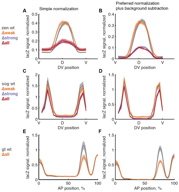
The expression patterns of zen (A and B), sog (C and D) and gt enhancers (E and F), and their variants are shown as line traces through the embryo. For zen and sog, the trace is around the circumference of the embryo; dorsal is in the middle, ventral is on the edges. For gt, the trace is along the lateral side of the embryo; anterior is left, posterior is right. In the gt plots, the anterior and posterior peaks are from the hkb co-stain. The average expression level is shown as a solid line, standard errors of the mean are shown as shaded areas in the corresponding color. In A, C, and E, measurements were normalized to the hkb levels directly. In B, D, and F, measurements were normalized to both lacZ and hkb levels, and we subtracted the background (see Results).

To remove influential outliers, we used the regstats command in MATLAB to calculate Cook’s distance, D [23]. Cook’s distance is an estimate of the influence of one point on the parameters of the regression.

$$D_i=\frac{\sum _{j=1}^n{\left({\widehat{Y}}_j-{\widehat{Y}}_{j(i)}\right)}^2}{p\mathrm{MSE}}$$

Here Ŷ_j is the prediction for observation j from the full linear regression, and Ŷ_j(i) is the prediction from a model fit without observation i. n is the total number of observations, p is the number of parameters in the model, and MSE is the mean square error of the model. We eliminated observations where D_i > 4/(n - 2) [24].

2.6 qPCR

For qPCR, we first cleared the population cages for at least 1 hour and then collected 2- 4 hour old embryos. We bleached the embryos in 50% bleach for 2 minutes and then snap-froze them in liquid nitrogen. We extracted total RNA using the protocol described in [25] with 50-100 uL of embryos and 500 uL TRIzol (Life Technologies; Grand Island, NY). We isolated the poly-A mRNA using the Oligotex kit (Qiagen; Germantown, MD) and performed reverse transcription using the SuperScript First-Strand Synthesis System for qPCR (Life Technologies) and 100 ng of poly-A mRNA. Using a 1:50 dilution of the resulting cDNA, we performed quantitative PCR using the TaqMan Universal PCR Master Mix and TaqMan Gene Expression Assays for lacZ and actin-5C (Life Technologies) as a housekeeping control. On an Eppendorf RealPlex² real time PCR machine, we ran a PCR program as follows: 95°C for 10 minutes, followed by 40 cycles of 95°C for 15 seconds and 60°C for 1 minute. Dilution curves confirmed that both these primer sets amplified with high efficiency. Threshold C_t values were determined automatically using the included Eppendorf software. For each reaction, we performed two technical replicates and averaged the resulting C_t values for a measurement. We calculated the ΔC_t value by subtracting the actin C_t from the lacZ C_t, and fold change between lacZ and actin as 2^-ΔCt. We normalized these values to the fold change of the line that expressed the lowest amount of lacZ to give us a fold change of lacZ between lines. We performed two biological replicates and calculated the standard error of the mean (SEM) of ΔC_t using these replicates. To calculate the error bars in lacZ-fold-change-space, we then performed the same calculations with ΔC_t ± SEM(ΔC_t).

3. Results

3.1 Test case

To test our ability to measure differences in mRNA levels using a co-stain approach, we created sets of transgenic lines that contain enhancers driving a lacZ reporter. To generate different reporter expression levels, we chose enhancers that are known or suspected to be activated by Zelda and mutated their Zelda binding sites. Zelda, also known as vielfaltig, is a ubiquitously-expressed transcription factor that binds to the enhancers of genes expressed soon after the maternal to zygotic transition in the Drosophila embryo [26]. The knockdown of Zelda decreases the expression level of many zygotically transcribed genes [27]. This effect has been verified in several specific loci using in situs, but the degree of this effect on expression level has not been quantified in these experiments [28,29]. We chose three enhancers for our test study, the zerknullt (zen) ventral expression element, the short gastrulation (sog) minimal enhancer and the giant (gt) posterior stripe enhancer. For each of these enhancers, we cloned the wild type sequence and sequences where Zelda sites have been mutated into non-sites to test our ability to measure changes in mRNA levels (Figure 1A). For two of these enhancers, the zen and sog enhancers, we made four lines: the wild type (wt) sequence, the sequence with weak sites mutated (Δweak), the sequence with strong sites mutated (Δstrong), and the sequence with all sites mutated (Δall). The gt enhancer does not contain any weak sites, so we made wt and Δall lines. We expected this set of sequences to drive different levels of lacZ mRNA expression. To verify our expectation, we performed qPCR experiments on the zen lines using 2-4 hour old embryos (Figure 1C). The qPCR experiments indicate lacZ levels are lowest in the Δall line, intermediate in the Δstrong and Δweak lines, and highest in the wt line.

Figure 1. A test set of transgenic reporters drives lacZ to different levels.

(A) To compare mRNA levels between different transgenic reporter lines, we stain embryos from these lines for the gene of interest, lacZ, and a co-stain, hkb, both in red, and DNA in green. Using a image processing pipeline, we can segment the image into cells. We then normalize the lacZ signal using the hkb co-stain and analyze the gene expression pattern, shown here as a line trace along the anterior-posterior axis of the embryo. (B-C) To test our ability to detect changes in mRNA levels, our goal was to create a set of transgenic reporters that drive lacZ to different levels. We selected a set of enhancers that contain binding sites for Zelda, a transcriptional activator. We identified predicted Zelda sites in each enhancer and mutated strong (Δstrong), weak (Δweak) or all (Δall) Zelda sites. In the diagrams, light pink circles are weak Zelda sites, and red circles are strong Zelda sites. For each enhancer, we created a transgenic D. melanogaster line with the enhancer driving lacZ. We show cartoons of the expression patterns of the wild-type enhancers in blastoderm-stage embryos. In the cartoons, anterior is left, posterior is right, dorsal up and ventral down. (D) qPCR results from the zen lines verify that deleting Zelda binding sites alters mRNA level. Results are plotted as fold change relative to the Δall lines. The error bars represent the standard error of the mean estimated from two biological replicates.

3.2 Selection of an appropriate co-stain

With this test set in hand, we then sought an appropriate co-stain for the experiments. An ideal co-stain has two properties: (1) it does not overlap in space with the expression pattern of interest, and (2) its expression level does not change dramatically between samples or over the time period of interest. It is possible to use a co-stain that somewhat overlaps the expression pattern of interest, but subsequent analyses would be limited to regions where there is no overlap between the primary stain and the co-stain. Expression levels can also vary somewhat over time, but this will limit the ability to accurately measure target gene expression levels. Our enhancers of interest drive expression patterns in the middle of the embryo (Figure 1B), so we chose a gene to co-stain that is expressed at the anterior and posterior ends of the embryo. huckebein (hkb), a gene in the terminal system fulfills both of these criteria (Figure 2A and C). We assume that the permeability of the embryo does not spatially vary; this assumption is supported by the uniformity of in situ stains for ubiquitously expressed genes [4,5].

Figure 2. The expression patterns of huckebein and our target genes do not overlap.

(A) On the top, we show a maximum intensity projection of an embryo at the beginning of the blastoderm stage of development stained for hkb expression (red) and DNA (green). Using an image processing pipeline to computationally align many embryos, we created a gene expression atlas that includes hkb expression [8]. The pose of the embryo is the same as in Fig. 1B. hkb is expressed in both the anterior and posterior of the embryo. (B) We show the expression pattern of hkb for half the embryo over the 6 time points in the atlas, using a rectangular projection and a heat map for expression levels. (C) We show the mean (dotted line) and 95% quantile values (solid line) of hkb expression in the anterior 10% (purple) and posterior 10% (orange) of the embryo. We chose the posterior region as our normalization domain because of the relative stability of hkb levels in time points 2 and 3.

Using a previously-published atlas of gene expression in the D. melanogaster embryo [5], we quantified the relative expression levels of hkb in the anterior 10% and posterior 10% of the embryo along the anterior-posterior axis. From this point on, we will call these regions the anterior section and the posterior section, and we will refer to the remaining 80% of the embryo as the middle section. This atlas contains relative gene expression measurements for six ten-minute time points during the blastoderm stage of development (Figure 2B). We used both the mean and the 95% quantile value to characterize the time trace of the hkb expression domains (Figure 2C). The posterior section has stable expression over two time points in this data, time points 2 and 3, while the anterior section changes more over time.

In choosing which time points to analyze, we realized that there is a tradeoff between the number of time points we analyze and accuracy because hkb expression changes over time. We perform all stains simultaneously to limit sources of experimental variability. Therefore, we had a finite number of embryos to analyze per sample and accordingly, a limited number of embryos from each ten-minute time point. Considering embryos in fewer time points decreases hkb level variability from embryo to embryo, but yields a smaller sample which increases measurement uncertainty. Conversely, considering embryos from more time points increases the sample size but also increases the variability in hkb level. Based on the sample sizes in this experiment, we chose to use embryos from time points 2 and 3 of the blastoderm stage, which roughly correspond to 10-30 minutes after the beginning of the blastoderm stage. We also chose the posterior domain of hkb as our normalization domain.

3.3 Co-stain is linearly correlated with stain of interest

Using embryos collected from the reporter lines shown in Figure 1, we carried out an in situ hybridization stain using mRNA probes for lacZ and hkb. We employ the in situ protocol and imaging conditions described in [22]. The most salient features of this protocol are the use of hapten-labeled RNA probes that we detect using antibodies that recognize these haptens. The antibodies contain a horseradish peroxidase domain that we use with a tyramide signal amplification kit to deposit a fluorescent dye. There is evidence from comparisons to antibody stains and directly labeled antibodies that this signal amplification is linear [22,30].

In our experiment, the lacZ and hkb probes were detected using the same color dye. All stains were done simultaneously, using the same batch of probes to reduce any variability resulting from differences in stain conditions. We imaged all embryos that were in time points 2 and 3. Using an image processing pipeline and a nuclear dye, the images are segmented into PointClouds, text files that contain the spatial coordinates of each nucleus in the embryo and the relative expression values of the stained genes.

The only requirement for our normalization scheme is that the levels of the co-stain must vary with the levels of the lacZ stain from embryo to embryo. If differences in stain brightness from embryo to embryo are due to differences in embryo permeability, we expect that hkb levels and lacZ levels will be linearly correlated between embryos of a particular genotype. If we plot lacZ levels versus hkb levels, we can fit a linear regression to determine the slope. We can then compare these slopes between transgenic lines to compare their lacZ levels. This strategy is based on the ratio of lacZ to hkb expression; it therefore does not depend on the relative hybridization efficiencies of the the lacZ and hkb probes. Our goal is to order the transgenic lines in terms of their slopes; any differences in probe efficiency will not impact the linearity of the lacZ/hkb relationship, and these differences will be consistent across all samples.

To assess the linearity of hkb/lacZ relationship, we do a linear regression of the hkb level measured in the posterior section and lacZ level measured in the middle of the embryo, where hkb is not expressed. To do this regression, we need to select appropriate measures of hkb and lacZ levels. The distributions of expression levels in the embryo are skewed towards small values, since the majority of cells in the embryo express neither hkb nor lacZ (Figure 3). We chose to use the 95% and 99% quantiles of expression as our metric of expression level; these statistics is more appropriate for skewed distributions than the mean. Moreover, quantiles are more robust to outliers than simply using the maximum expression value. The posterior section of the embryo contains ~400 cells of the 6000 total cells in the embryo, most of which express hkb. Therefore the 95% quantile corresponds to the ~20th brightest cell. The middle section of the embryo contains ~5000 cells, and the fraction expressing lacZ depends on the reporter. We estimate that at least 5-10% of the cells are expressing lacZ, and therefore use the 99% quantile, or the ~50th brightest cell, as our metric for lacZ. The particular quantile value, e.g. 95% or 99%, is arbitrary; we selected these values as we were confident that they would fall in the part of the distribution of cells that are expressing either lacZ or hkb.

Figure 3. Quantile measurements capture representative levels of expression.

Here we show the distribution of hkb and lacZ expression values in each cell for three sample embryos from the zen Δall line. Note that the scale of expression differs across these plots, supporting the need for normalization to calibrate measured expression values. When plotted for all cells (left), the peak in the distribution near zero represents cells expressing neither hkb nor lacZ, and the width and location correlates with the degree of experimental noise in our measurements. When plotted for the posterior (middle column) and middle domains (right column), the distributions are also asymmetric, supporting the use of quantiles to characterize the levels of hkb and lacZ expression consistently across transgenic lines (orange lines). Note that the quantiles select a similar part of the distribution in every embryo, while the mean would be influenced by the varying shapes of the distributions.

With these two metrics, we ran a linear regression. We removed influential outliers using a standard distance metric (Material and Methods). In Table 1, we report the number of embryos and correlation coefficient before and after trimming the samples of outliers. We find all lines show a moderate to strong correlation between the hkb and lacZ levels (r > 0.71, after trimming), and the trimming generally increases the correlation coefficient, while reducing the sample size by ~10%. In Figure 4, we show plots of lacZ levels versus hkb levels and the residual plots resulting from the fit. These plots and the test statistics indicate that the linear model is appropriate.

Table 1.

Summary statistics of the linear regression between hkb and lacZ levels

	Line	n	r	nTrimmed	rTrimmed	slope±95% CI	F-statistic p-value
zen	wt	30	0.94	27	0.96	0.67±0.083	5E-12
	Δweak	26	0.96	24	0.94	0.63±0.10	7E-12
	Δstrong	20	0.97	19	0.98	0.33±0.034	2E-13
	Δall	5	0.88	4	0.98	0.32±0.21	0.023
sog	wt	20	0.58	18	0.80	1.4±0.58	8E-05
	Δweak	26	0.93	23	0.88	1.8±0.45	4E-08
	Δstrong	35	0.85	31	0.87	1.6±0.35	2E-10
	Δall	28	0.92	26	0.73	1.4±0.54	3E-05
gt	wt	17	0.82	15	0.71	1.7±0.72	2E-04
	Δall	23	0.91	21	0.78	0.99±0.37	3E-05

Here we report the number of embryos (n), correlation coefficient (r), slopes, confidence intervals (CI), and F-statistic p-values for the regression of hkb and lacZ levels. The nTrimmed, rTrimmed, slope and F-statistic p-values are reported for the data after trimming using Cook’s distance.

Figure 4. Huckebein and lacZ levels are correlated within a genotype.

In the first column (A, C, E), we compare the expression levels of hkb (the 95% quantile of expression levels in the posterior of the embryo) to lacZ (the 99% quantile of the expression levels in the middle of the embryo). The points are colored according to reporter construct, and we fit a line to the results from each reporter (colored lines). In the second column (B, D, F), we plot the standardized residuals, which are the deviations of each data point from the fitted line. These plots indicate that the linear fit is appropriate because the residual scatter is roughly equally spread between values above and below zero without any particular pattern.

Given this correlation, we can now quantitatively compare mRNA levels between lines using our imaging data. Steeper slopes of the line relating hkb and lacZ levels indicate higher lacZ levels; we find that the zen lines show a clear decrease in lacZ levels upon the deletion of strong Zelda sites. The qPCR experiment shown in Figure 1C also clearly shows a difference in expression level between the WT and Δall lines. Moreover, the relative ordering of the lines is the same using either the imaging or qPCR data. However, the statistical significance of the differences between each line are different between the two methods, as one might expect: qPCR is done with material from a much larger time window than the ten-minute resolution of the imaging experiment.

We examined two other enhancers, gt and sog, using this slope metric. The two gt lines, wt and Δall, also show a decrease in lacZ level upon Zelda site deletion. The sog lines do not show significant changes in slope, but do show differences in expression level when the spatially resolved patterns are examined, as discussed below.

3.4 Normalization to allow for spatially resolved signals

Once we have confirmed that the co-stain varies with lacZ, we can then use co-stain levels to normalize our measurements in each cell. As stated earlier, we assume that embryo-to-embryo variability is due to changes in embryo permeability, and we verified that hkb levels are correlated with lacZ levels in each line. In order to normalize measurements on a cell-by-cell basis, the simplest approach is to each cell’s expression level by hkb level, and then carry out any subsequent analysis. We tried this approach and then created line traces to get spatially resolved comparisons of lacZ levels between embryos (Figure 5A, C, E). We also plot the standard error of the mean of these line traces. These error bars are an estimate of both the biological and measurement noise in the experiment. These results generally agree with the slope comparisons, but the addition of spatial resolution allows for a more nuanced comparison of the changes in the expression patterns caused by the Zelda site deletions. For the zen lines, the expression domain is similar between lines, and the Δstrong and Δlines show markedly lower lacZ levels than the wt and Δweak lines. In sog lines, we can now see small decreases in lacZ levels in the Δweak, Δstrong, and Δall lines as compared to the wt line. The Δall gt line shows a decrease relative to the wt line.

To take advantage of more of the data to estimate embryo permeability, we can apply a more sophisticated normalization technique. When we fit a line to the hkb versus lacZ levels, we see a scatter. This scatter is caused by several factors: measurement error, changes in lacZ and hkb levels over time, and embryo-to-embryo variability in lacZ and hkb levels. By normalizing strictly by hkb level, we are implicitly assuming that it is less variable between embryos than lacZ, an assumption we do not have evidence for. A more unbiased approach would be to use both the hkb and lacZ levels to determine permeability. For each line, we assume

$$\begin{array}{l}\mathrm{measured‐hkb}(\mathrm{i})=\mathrm{p}(\mathrm{i})•\mathrm{actual‐hkb}\\ \mathrm{measured‐lacZ}(\mathrm{i})=\mathrm{p}(\mathrm{i})•\mathrm{actual‐lacZ}\end{array}$$

Here measured-hkb(i) is the measured level of hkb in embryo i, measured-lacZ(i) is the measured level of lacZ in embryo i, and p(i) is the permeability of embryo i. actual-hkb is the absolute level of hkb in the embryo and actual-lacZ is the absolute level of lacZ in the embryo. Our linear regression indicates that, within a transgenic line:

$$\mathrm{measured‐hkb}(\mathrm{i})•\mathrm{m}+\mathrm{b}=\mathrm{measured‐lacZ}(\mathrm{i})$$

The constant b is not significantly different from 0 for any of our lines, so we drop it from the equation. (In fact, we also refit the linear regression between hkb and lacZ, forcing the constant b to 0 and found this regression yielded slightly higher r² values, but no qualitative change in our results.) Therefore, we can estimate permeability within a multiplicative constant (actual-hkb) in two ways:

$$\begin{array}{l}\mathrm{p}(\mathrm{i})•\mathrm{actual‐hkb}=\mathrm{measured‐hkb}(\mathrm{i})\\ \mathrm{p}(\mathrm{i})•\mathrm{actual‐hkb}=\mathrm{measured‐lacZ}(\mathrm{i})/\mathrm{m}\end{array}$$

We assume that measured-hkb(i) and measured-lacZ(i) are equally accurate measurements, so we estimate

$$\mathrm{p}(\mathrm{i})=(\mathrm{measured‐hkb}(\mathrm{i})+\mathrm{measured‐lacZ}(\mathrm{i})/\mathrm{m})/2$$

From Figure 5A, C, E, we also notice that the background varies from embryo to embryo, so we additionally subtract the minimum value of the line trace to set the background equal to 0.

This slightly more intricate normalization procedure creates a trade-off in which the error bars around the hkb levels widen while the error bars around the lacZ levels narrow but does not qualitatively change the results of the study (Figure 5 B, D).

4. Discussion

Here we present a technique to detect quantitative, spatially resolved changes in mRNA levels. This technique is easy to apply; it uses a typical in situ protocol and straightforward analysis techniques. The primary benefit is that the resulting mRNA levels can be compared in a statically rigorous fashion. Though here we perform our analysis using cellular resolution data, this is not a prerequisite for the approach. One could easily carry out the same techniques using pixels instead of cells as a measurement unit.

Our technique has two requirements. First, it requires the same pair of probes to be used across samples, one for the target gene and one for the co-stained gene. This pair must be the same because the analysis relies on the ratio of signal from the probe pair. If the hybridization efficiency differs between samples, this ratio will not be reliable. For example, if you are comparing the expression of orthologous genes across species, either probe may not have the exact same sequence and thus have a different hybridization efficiency. Second, our method requires selection of an appropriate gene to co-stain. Ideally, the expression pattern of the co-stained gene does not overlap the expression pattern of the target gene; the degree of expression pattern overlap influences the number of cells that can be analyzed. The ideal gene to co-stain also does not vary in level between samples at equivalent time points. A systematic difference in the level of co-stain expression between samples would confound the relative measurement of target gene expression levels. This may be important when considering comparison across different genotypes, where trans-effects are expected.

Our method is semi-quantitative, but easy to employ. Several other techniques yield absolute measurements of mRNA levels by counting individual transcripts, but in general are more difficult or expensive to apply. One strategy uses a pool of labeled DNA probes that target non-overlapping parts of the same gene to count single mRNA molecules [10-12,14,15]. The stained tissue is then imaged, and spot counting algorithms yield estimates of absolute numbers of mRNA molecules. Other techniques use single long mRNA probes and similar spot counting techniques [13,16], but require careful controls to ensure that each spot corresponds to a single mRNA.

By quantitating the expression patterns driven by our test set, we gained several new insights into Zelda function. Our test set comprised reporter constructs driven by enhancers with differing numbers of Zelda sites. Zelda, or vielfaltig, is a ubiquitously-expressed transcriptional activator; disruption of Zelda binding sites in enhancers is known to influence gene expression levels [28,29]. First, the impact of deleting all Zelda sites varies between different enhancers, though notably, all of the enhancers we chose bind Zelda in vivo [26]. This emphasizes that though many enhancers have been shown to bind Zelda [26,31,32], enhancers have different degrees of dependence on Zelda for their function. This agrees with the observations from [27], which also showed that genes are differentially affected by Zelda knockdown. In whole genome experiments, some of these effects may be indirect; our reporter constructs indicate that at least for the three genes studied here, the effects are direct. Second, even when we deleted all the Zelda sites from each enhancer, there was still detectable lacZ expression. This indicates that Zelda is not absolutely required for gene expression driven by these enhancers. Finally, for the sog and zen enhancers, we found that deleting weak Zelda sites had little impact on overall expression levels, indicating that stronger sites are more functionally important. This is consistent with the observation that strong Zelda binding correlates with larger expression changes upon Zelda depletion [26].

With current methods, there is a trade-off between quantitation and spatial resolution in measuring gene expression. In situ hybridization and other imaging-based techniques can measure mRNA expression with high spatial and temporal resolution for small numbers of genes, but are not quantitative without internal standards or counting of individual transcripts. Genome-wide techniques like RNA-seq yield highly quantitative measures of mRNA levels, but are not spatially resolved because they require large amounts of material, most often from homogenized tissues. Because of the large amounts of material required, multiple embryos are usually processed together, limiting temporal resolution and obscuring embryo-to-embryo variability. Clearly, the ideal will bring the best of both these techniques: quantitative, genome-wide data at high spatial and temporal resolution. In the interim, it is useful to bring quantitation to standard spatially resolved techniques, such as in situ hybridization; that was our goal with this work. Improvements are also occurring from the other direction: recent work has reduced the sample size required for RNA-seq to single embryo [33] and sub-embryo sizes [34]. Because quantitative, spatially resolved data is a requirement for modeling the behavior of developmental networks, we are optimistic that the field will continue to press forward on this problem.

• *we introduce a technique to compare mRNA levels of the same gene between samples
• *this technique can be used in the context of a typical in situ protocol
• *we compare D. melanogaster lines driving a reporter gene to differing levels
• *we detect spatially resolved differences in mRNA levels in embryos from these lines

List of abbreviations

CI

confidence interval

SEM

standard error of the mean

wt

wild type

References

- 1.Darby IA, Hewitson TD. Situ Hybridization Protocols (Methods in Molecular Biology) Humana Press; 2010. [Google Scholar]
- 2.Levsky JM, Singer RH. Fluorescence in situ hybridization: past, present and future. J Cell Sci. 2003;116:2833–2838. doi: 10.1242/jcs.00633. [DOI] [PubMed] [Google Scholar]
- 3.de Boer BA, Ruijter JM, Voorbraak FP, Moorman AF. More than a decade of developmental gene expression atlases: where are we now? Nucleic Acids Res. 2009;37:7349–7359. doi: 10.1093/nar/gkp819. [DOI] [PMC free article] [PubMed] [Google Scholar]
- 4.Tomancak P, et al. Systematic determination of patterns of gene expression during Drosophila embryogenesis. Genome Biol. 2002;3:RESEARCH0088. doi: 10.1186/gb-2002-3-12-research0088. [DOI] [PMC free article] [PubMed] [Google Scholar]
- 5.Fowlkes CC, et al. A quantitative spatiotemporal atlas of gene expression in the Drosophila blastoderm. Cell. 2008;133:364–374. doi: 10.1016/j.cell.2008.01.053. [DOI] [PubMed] [Google Scholar]
- 6.Fowlkes CC, et al. A conserved developmental patterning network produces quantitatively different output in multiple species of Drosophila. PLoS Genet. 2011;7:e1002346. doi: 10.1371/journal.pgen.1002346. [DOI] [PMC free article] [PubMed] [Google Scholar]
- 7.Lecuyer E, et al. Global analysis of mRNA localization reveals a prominent role in organizing cellular architecture and function. Cell. 2007;131:174–187. doi: 10.1016/j.cell.2007.08.003. [DOI] [PubMed] [Google Scholar]
- 8.Luengo-Oroz MA, Ledesma-Carbayo MJ, Peyrieras N, Santos A. Image analysis for understanding embryo development: a bridge from microscopy to biological insights. Curr Opin Genet Dev. 2011;21:630–637. doi: 10.1016/j.gde.2011.08.001. [DOI] [PubMed] [Google Scholar]
- 9.Dunipace L, Ozdemir A, Stathopoulos A. Complex interactions between cis-regulatory modules in native conformation are critical for Drosophila snail expression. Development. 2011;138:4075–4084. doi: 10.1242/dev.069146. [DOI] [PMC free article] [PubMed] [Google Scholar]
- 10.Femino AM, Fay FS, Fogarty K, Singer RH. Visualization of single RNA transcripts in situ. Science. 1998;280:585–590. doi: 10.1126/science.280.5363.585. [DOI] [PubMed] [Google Scholar]
- 11.Zenklusen D, Larson DR, Singer RH. Single-RNA counting reveals alternative modes of gene expression in yeast. Nat Struct Mol Biol. 2008;15:1263–1271. doi: 10.1038/nsmb.1514. [DOI] [PMC free article] [PubMed] [Google Scholar]
- 12.Raj A, van den Bogaard P, Rifkin SA, van Oudenaarden A, Tyagi S. Imaging individual mRNA molecules using multiple singly labeled probes. Nat Methods. 2008;5:877–879. doi: 10.1038/nmeth.1253. [DOI] [PMC free article] [PubMed] [Google Scholar]
- 13.Pare A, et al. Visualization of individual Scr mRNAs during Drosophila embryogenesis yields evidence for transcriptional bursting. Curr Biol. 2009;19:2037–2042. doi: 10.1016/j.cub.2009.10.028. [DOI] [PMC free article] [PubMed] [Google Scholar]
- 14.Little SC, Tkacik G, Kneeland TB, Wieschaus EF, Gregor T. The formation of the Bicoid morphogen gradient requires protein movement from anteriorly localized mRNA. PLoS Biol. 2011;9:e1000596. doi: 10.1371/journal.pbio.1000596. [DOI] [PMC free article] [PubMed] [Google Scholar]
- 15.Itzkovitz S, van Oudenaarden A. Validating transcripts with probes and imaging technology. Nat Methods. 2011;8:S12–9. doi: 10.1038/nmeth.1573. [DOI] [PMC free article] [PubMed] [Google Scholar]
- 16.Boettiger AN, Levine M. Rapid transcription fosters coordinate snail expression in the Drosophila embryo. Cell Rep. 2013;3:8–15. doi: 10.1016/j.celrep.2012.12.015. [DOI] [PMC free article] [PubMed] [Google Scholar]
- 17.Gibson DG, et al. Enzymatic assembly of DNA molecules up to several hundred kilobases. Nature methods. 2009;6:343–345. doi: 10.1038/nmeth.1318. [DOI] [PubMed] [Google Scholar]
- 18.Satija R, Bradley RK. The TAGteam motif facilitates binding of 21 sequence-specific transcription factors in the Drosophila embryo. Genome Res. 2012;22:656–665. doi: 10.1101/gr.130682.111. [DOI] [PMC free article] [PubMed] [Google Scholar]
- 19.Hare EE, Peterson BK, Iyer VN, Meier R, Eisen MB. Sepsid even-skipped enhancers are functionally conserved in Drosophila despite lack of sequence conservation. PLoS Genet. 2008;4:e1000106. doi: 10.1371/journal.pgen.1000106. [DOI] [PMC free article] [PubMed] [Google Scholar]
- 20.Fish MP, Groth AC, Calos MP, Nusse R. Creating transgenic Drosophila by microinjecting the site-specific phiC31 integrase mRNA and a transgene-containing donor plasmid. Nat Protoc. 2007;2:2325–2331. doi: 10.1038/nprot.2007.328. [DOI] [PubMed] [Google Scholar]
- 21.Groth AC, Fish M, Nusse R, Calos MP. Construction of transgenic Drosophila by using the site-specific integrase from phage phiC31. Genetics. 2004;166:1775–1782. doi: 10.1534/genetics.166.4.1775. [DOI] [PMC free article] [PubMed] [Google Scholar]
- 22.Luengo Hendriks CL, et al. Three-dimensional morphology and gene expression in the Drosophila blastoderm at cellular resolution I: data acquisition pipeline. Genome Biol. 2006;7:R123. doi: 10.1186/gb-2006-7-12-r123. [DOI] [PMC free article] [PubMed] [Google Scholar]
- 23.Cook RD. Detection of Influential Observation in Linear Regression. Technometrics. 1977;19:15–18. [Google Scholar]
- 24.Sheather S. A Modern Approach to Regression with R (Springer Texts in Statistics) Springer; 2009. [Google Scholar]
- 25.B K, A J. Extraction of Total RNA from Drosophila. 2006 CGB Technical Report 2006-10. [Google Scholar]
- 26.Harrison MM, Li X-Y, Kaplan T, Botchan MR, Eisen MB. Zelda binding in the early Drosophila melanogaster embryo marks regions subsequently activated at the maternal-to-zygotic transition. PLoS genetics. 2011;7:e1002266. doi: 10.1371/journal.pgen.1002266. [DOI] [PMC free article] [PubMed] [Google Scholar]
- 27.Liang HL, et al. The zinc-finger protein Zelda is a key activator of the early zygotic genome in Drosophila. Nature. 2008;456:400–403. doi: 10.1038/nature07388. [DOI] [PMC free article] [PubMed] [Google Scholar]
- 28.Liberman LM, Stathopoulos A. Design flexibility in cis-regulatory control of gene expression: synthetic and comparative evidence. Dev Biol. 2009;327:578–589. doi: 10.1016/j.ydbio.2008.12.020. [DOI] [PMC free article] [PubMed] [Google Scholar]
- 29.ten Bosch JR, Benavides JA, Cline TW. The TAGteam DNA motif controls the timing of Drosophila pre-blastoderm transcription. Development. 2006;133:1967–1977. doi: 10.1242/dev.02373. [DOI] [PubMed] [Google Scholar]
- 30.Wunderlich Z, et al. Dissecting sources of quantitative gene expression pattern divergence between Drosophila species. Mol Syst Biol. 2012;8:604. doi: 10.1038/msb.2012.35. [DOI] [PMC free article] [PubMed] [Google Scholar]
- 31.Kvon EZ, Stampfel G, Yanez-Cuna JO, Dickson BJ, Stark A. HOT regions function as patterned developmental enhancers and have a distinct cis-regulatory signature. Genes Dev. 2012;26:908–913. doi: 10.1101/gad.188052.112. [DOI] [PMC free article] [PubMed] [Google Scholar]
- 32.Nien CY, et al. Temporal coordination of gene networks by Zelda in the early Drosophila embryo. PLoS Genet. 2011;7:e1002339. doi: 10.1371/journal.pgen.1002339. [DOI] [PMC free article] [PubMed] [Google Scholar]
- 33.Lott SE, et al. Noncanonical compensation of zygotic X transcription in early Drosophila melanogaster development revealed through single-embryo RNA-seq. PLoS Biol. 2011;9:e1000590. doi: 10.1371/journal.pbio.1000590. [DOI] [PMC free article] [PubMed] [Google Scholar]
- 34.Combs P, Eisen MB. Sequencing mRNA from Cryo-Sliced Drosophila Embryos to Determine Genome-Wide Spatial Patterns of Gene Expression. PLoS One. 2013;8:e71820. doi: 10.1371/journal.pone.0071820. [DOI] [PMC free article] [PubMed] [Google Scholar]
Associated Data
This section collects any data citations, data availability statements, or supplementary materials included in this article.