Detecting phase-amplitude coupling with high frequency resolution using adaptive decompositions

Abstract

Background

Phase-amplitude coupling (PAC) – the dependence of the amplitude of one rhythm on the phase of another, lower-frequency rhythm – has recently been used to illuminate cross-frequency coordination in neurophysiological activity. An essential step in measuring PAC is decomposing data to obtain rhythmic components of interest. Current methods of PAC assessment employ narrowband Fourier-based filters, which assume that biological rhythms are stationary, harmonic oscillations. However, biological signals frequently contain irregular and nonstationary features, which may contaminate rhythms of interest and complicate comodulogram interpretation, especially when frequency resolution is limited by short data segments.

New method

To better account for nonstationarities while maintaining sharp frequency resolution in PAC measurement, even for short data segments, we introduce a new method of PAC assessment which utilizes adaptive and more generally broadband decomposition techniques – such as the empirical mode decomposition (EMD). To obtain high frequency resolution PAC measurements, our method distributes the PAC associated with pairs of broadband oscillations over frequency space according to the time-local frequencies of these oscillations.

Comparison with existing methods

We compare our novel adaptive approach to a narrowband comodulogram approach on a variety of simulated signals of short duration, studying systematically how different types of nonstationarities affect these methods, as well as on EEG data.

Conclusions

Our results show: (1) narrowband filtering can lead to poor PAC frequency resolution, and inaccuracy and false negatives in PAC assessment; (2) our adaptive approach attains better PAC frequency resolution and is more resistant to nonstationarities and artifacts than traditional comodulograms.

1. Introduction

Complex biological systems contain rhythmic components at multiple frequencies, and these rhythms are rarely independent, exhibiting many forms of coupling including phase synchronization and amplitude comodulation (Rosenblum et al., 1997; Tass et al., 1998; Fries, 2005; Womelsdorf et al., 2007; Lo et al., 2008; Sauseng et al., 2008; Darvas et al., 2009; Fell and Axmacher, 2011; Bartsch et al., 2012; Hu et al., 2012; Schutter and Knyazev, 2012). Recently, a great deal of attention has been paid to phase-amplitude coupling (PAC) in neuronal signals, in which two rhythms co-exist and the amplitude of the higher frequency rhythm itself oscillates in phase with the lower frequency rhythm (Lakatos et al., 2005; Buszaki, 2006; Jensen and Colgin, 2007; Cohen et al., 2009; Canolty and Knight, 2010; Axmacher et al., 2010). For instance, there is extensive evidence of phase-amplitude coupling between theta (~4–10 Hz) and gamma (~40–100 Hz) rhythms in electroencephalogram (EEG) and local field potential (LFP) recordings (Bragin et al., 1995; Canolty et al., 2006; Montgomery et al., 2008; Sirota et al., 2008; Tort et al., 2009; Scheffzuk et al., 2011). This PAC is empirically linked both to neuronal circuit dynamics and to cognitive processes, and is believed to reflect neural coding and information transfer within the complex neural network of the brain (Jensen and Lisman, 1996; von Stein and Sarnthein, 2000; Lakatos et al., 2005; Jensen and Colgin, 2007; Cohen et al., 2009; Canolty and Knight, 2010; Axmacher et al., 2010). In addition, PAC phenomena have been observed in other complex systems in geology and finance (Rennert and Wallace, 2009; He et al., 2010). Thus, PAC and other types of cross-frequency coupling may serve as generic, promising tools for investigating the multiscale interactions underlying complex systems (He et al., 2010).

Reliable estimation of PAC requires not only identifying the existence of certain rhythms by their average spectral power, but also determining the precise profiles of individual cycles of these rhythms. Thus, neurophysiological time series present a number of challenges for PAC assessment: their multiple component oscillations may be buried under complex and nonstationary noise, may be present only intermittently, and may exhibit seemingly unstable waveforms varying in amplitude and frequency. Thus, the frequency domain representations of neural signals – like the underlying neural activity they measure – are broadband, even when rhythms of interest are not, and decomposing data to extract these rhythms is far from trivial. The Fourier transform can introduce non-physiological oscillations to account for nonsinusoidal and nonstationary properties of these signals (Kramer et al., 2008; Lo et al., 2009a), a difficulty that may be aggravated in short time series, for which frequency resolution (as measured by the Rayleigh resolution – the difference between consecutive frequencies represented in the Fourier transform) is severely limited.

To address some of these issues, we introduce a novel PAC measurement method which couples a broadband, adaptive decomposition method – the empirical mode decomposition (EMD) (Huang et al., 1998) – with time-local frequency assessment. The EMD iteratively applies a procedure called “sifting” to extract the fastest timescale fluctuations from a signal, resulting in a series of successively lower-frequency oscillatory components called intrinsic mode functions (IMFs). The original signal can be represented as the sum of these IMFs, each of which is unique to the data. As the IMFs are derived in the time domain without the assumption of constant frequency, amplitude, and functional form, each IMF may be frequency- and/or amplitude-modulated.

Due to the broadband and data-derived nature of these IMFs, combining current methods with the EMD or another adaptive decomposition would yield, at best, PAC measurements with very broad frequency resolution (i.e., PAC measurements computed between oscillations with energy over a wide range of frequencies), and at worst, PAC measurements incomparable between data segments (i.e., PAC measurements computed between oscillations with frequency content that is highly variable between data segments). Our method, called Intrinsic Mode Phase-Amplitude Coupling (IMPAC), resolves this issue. It calculates a measure of phase-amplitude coupling between each IMF and its higher-frequency IMFs. Rather than assigning this measure to a single frequency pair, determined by, for instance, the average frequency content of the phase-giving and amplitude-giving IMFs, IMPAC redistributes the calculated coupling across the phase frequency-amplitude frequency plane. This redistribution is done according to the proportion of time the two IMFs spend at each phase frequency-amplitude frequency coordinate, as determined by the cycle-by-cycle frequencies of the two IMFs.

While IMPAC is built around the EMD, similar approaches may be implemented on the output of any adaptive or otherwise broadband decomposition method, such as wavelet decomposition. As an illustration, we have applied the IMPAC approach to the output of a serial, dyadic filter bank with an average frequency response similar to the EMD (Flandrin et al., 2003, 2005; Wu and Huang, 2004) and many similarities to the wavelet transform, a method we call the Dyadic Filter bank PAC method (DFPAC).

We compared the performance of IMPAC and DFPAC to two standard Fourier-based PAC methods on both simulated signals and real EEG data. Our simulated signals contained PAC at frequencies chosen to mimic theta and gamma rhythms in brain activity – the phase of a 6 Hz rhythm modulates the amplitude of a 65 Hz rhythm – as well as a number of data processing challenges that are often present in neurophysiological data: measurement noise; missing data; random trends or measurement drift; the presence of uncoupled, frequency- and amplitude-modulated oscillations; and coupled oscillations with amplitude proportional to frequency. The coupled rhythms were for the most part stationary and sinusoidal, but we also examined frequency-modulated and asymmetric coupled oscillations. We simulated a total of 150 s of signal for each challenge, divided into 3 s epochs. Each epoch was designed to capture the same system – i.e., there is some stationarity across epochs – and we measured the average performance of each measure on the 50 epochs. We also tested all PAC measurement methods on mouse intracranial EEG recorded during REM sleep, a state in which brain signals have been shown to exhibit robust theta-gamma PAC (Scheffzuk et al., 2011), as well as multiple nonstationarities and artifacts in combination.

Our results show that, perhaps counter intuitively, standard comodulograms can yield poor frequency resolution of PAC, inaccurate PAC frequency assignment, and false negatives in PAC assessment. The novel strategy of recovering PAC from broadband oscillations and determining its frequency characteristics time-locally and post-decomposition attains better PAC frequency resolution and is more resistant to the effects of nonstationari-ties than standard comodulograms. We also obtain novel results regarding the effects of uncoupled oscillations. While these uncoupled rhythms a priori should not affect PAC measurement, we show that they distort both narrow- and broadband PAC measurements in characteristic ways, suggesting differential use of these approaches to minimize the effects of constant-frequency vs. frequency-modulated uncoupled oscillations.

2. Methods

2.1. PAC quantification

Several methods of exploring PAC have been employed in the literature. One popular analysis is the comodulogram, in which a “coupling palette” is computed and used to indicate, for wide ranges of phase-giving and amplitude-giving frequencies, the strength of the modulation of amplitude by phase (Tort et al., 2008, 2009; Scheffzuk et al., 2011). The advantage of the comodulogram is that it allows the experimentalist to see at a glance the phase-and amplitude-giving frequencies that exhibit strong coupling; only ranges of possibly coupled frequencies must be chosen before analysis.

There are five steps in computing the comodulogram: (1) decomposing the time series of interest to isolate a high frequency amplitude-giving rhythm S_a at frequency f_a and a low frequency phase-giving rhythm S_p at frequency f_p (Fig. 1A and B); (2) obtaining the instantaneous phase Φ_p of S_p and the instantaneous amplitude A_a of S_a (Fig. 1B); (3) quantifying the dependence of A_a on Φ_p (Fig. 1C); (4) determining the significance of this dependence, usually using a test of surrogate data; and (5) repeating these measures for multiple pairs (f_p, f_a) (Fig. 2A and B).

Fig. 1.

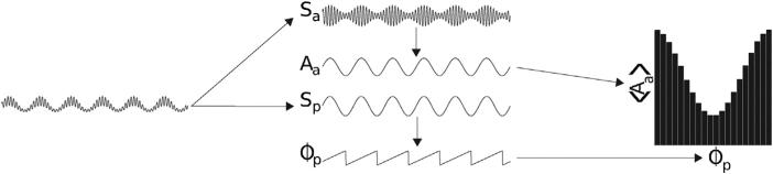
Phase-amplitude dependence. The basic approach to measuring PAC, illustrated with a simple signal exhibiting phase-amplitude coupling (A). The signal is filtered into two frequency components of interest: an amplitude-giving signal S_a and a phase-giving signal S_p, and their respective amplitude time series A_a and phase time series Φ_p are extracted (B). The amplitudes A_a(t) are averaged in bins according to the phase Φ_p(t), resulting in a phase-amplitude distribution (C). The difference of this phase-amplitude distribution from a uniform (flat) distribution is quantified, and indicates the amount of phase-amplitude coupling in the time series.

Fig. 2.

The comodulogram. Filtering a signal into many frequency bands, computing the distribution of amplitude by phase for each pair of signals, and quantifying the uniformity of these distributions results in a comodulogram (A). To determine whether the resulting modulation index is significant, surrogate data is used to estimate null distributions for each pair of phase- and amplitude-giving signals, and these null distributions are used to threshold the observed modulation indices (B). For IMPAC and DFPAC, we proceed to redistribute the IE between each pair of signals in the phase frequency-amplitude frequency plane (C), and average over each bin in this plane to obtain our final comodulogram (D).

For the standard comodulograms, we followed most of the details in (He et al., 2010), applying third-order Butterworth filters and the Hilbert transform to obtain the instantaneous amplitude and phase of various oscillatory signal components, and using an inverse entropy (IE) measure based on the Kullback-Liebler distance to quantify phase-amplitude dependence between components (Tort et al., 2010). To explore how the frequency and time resolution tradeoff affects PAC measurement, we implemented filters with two rolloff characteristics – shallow (–60 dB per decade, BPAC1) and steep (<–350 dB per decade, BPAC2) – for low-frequency passbands of width 0.4 Hz, centered every 0.4 Hz from 3.2 Hz to 8.8 Hz, and high-frequency passbands of width 6 Hz, centered every 6 Hz from 23 Hz to 107 Hz. The width of these phase-giving passbands is close to the Rayleigh resolution of our simulated data (1/600 = 0.33 Hz), but a set of analyses with 2 Hz phase-giving passbands yields similar results to those described for both our simulations and our experimental data (Appendix A). In calculating the null distribution of IE for each frequency pair, we used a new surrogate data method, described below. The resulting IE distribution was used to z-score the observed IE, and these z-scores were then thresholded, so that those not exceeding a significance level of p = 0.05 (Bonferroni-corrected over all tested pairs of phase-giving and amplitude-giving components) were ignored.

IMPAC introduces modifications to the first and third steps, as well as two novel steps: (2a) computation of cycle-by-cycle frequency time series F_p and F_a for both S_p and S_a; and (6) computation of a high frequency resolution comodulogram using this cycle-by-cycle frequency information. We discuss these modifications below.

2.1.1. Signal decomposition using ensemble EMD

The EMD decomposes a time series into a small number of intrinsic mode functions, or IMFs (Huang et al., 1998), derived in the time domain without the assumption of constant frequency, amplitude, and functional form. Typically the number of IMFs is on the order of the base-2 logarithm of the signal length, with slight variations depending on the complexity of the signal. These IMFs are “oscillation-like” in the following way: the absolute difference between the number of zero-crossings and the number of local extrema is no more than one; and the mean value of each IMF is close to zero except for the last IMF that describes the global trend of the time series.

The latter notion is the one used to implement the EMD, through a process called “sifting”. In sifting, the local maxima and minima of the time series are spline-interpolated to create an “upper envelope” and a “lower envelope” time series, respectively. The upper and lower envelopes are then averaged, and this nonstationary trend is subtracted from the data, leaving behind the maxima and minima that constitute the fastest fluctuations in the signal. This process is repeated until the average of the upper and lower envelopes is uniformly smaller than a given tolerance. The result is the first IMF extracted from the signal. It exhibits the component oscillations which are of highest frequency locally in time. This first IMF can be subtracted from the time series to yield a residual. This residual can in turn be sifted to yield a second IMF, containing component oscillations that are lower in frequency than those exhibited in IMF 1, at least locally in time. The process continues iteratively until the residual is monotonic and can no longer be sifted.

While the EMD is neither linear nor a frequency-domain decomposition, some intuition into its behavior can be gained from asking what kinds of linear, frequency domain filters it is most like. This has been assessed by applying the EMD to a large number of realizations of colored noise, and averaging together the Fourier spectra of the resulting IMFs (Flandrin et al., 2003, 2005; Wu and Huang, 2004). The resulting frequency responses of the first 10 IMFs suggest that, at least on colored noise signals, the EMD acts roughly like a serial, dyadic, high-pass filter bank. What this means is that the first IMF contains approximately the top half of the frequency content of the noise; the second IMF contains the next quarter of the frequency content; the third IMF contains the next eighth, and so on. Thus, if the EMD yields 10 IMFs, the last 7 of these will represent the lowest eighth of the signal's frequency content.

One of the difficulties of the EMD is that it can be sensitive to small changes in the values of a time series. For example, low pass filtering may alter the results of the EMD: if the EMD decomposes a signal into 10 IMFs, the first five of which have frequency content above 200 Hz, one might hope that applying the EMD after low-pass filtering the signal at 200 Hz would recover the last five IMFs from the original decomposition, but this may not be the case. A refinement of the EMD, known as ensemble empirical mode decomposition (EEMD; Wu and Huang, 2009), can help to address this issue. In the EEMD, one performs the empirical mode decomposition on an ensemble of signals, obtained from the original signal by adding multiple realizations of white noise, and then averages these decompositions together, resulting in more stable and cleaner decompositions. For each signal of interest, we performed EEMD on an ensemble of 100 signals with added white noise having variance 0.1. Thus, the standard deviation of the Gaussian distributed noise present in the sum of all components of the EEMD decomposition is ~1% of the standard deviation of the raw signal. In this study IMFs having fewer than 5 cycles were discarded. We calculated the IE of the phase of IMF n on the amplitude of (higher frequency) IMFs n – 1, n – 2,. . ., 2, and 1.

2.1.2. Signal decomposition using a dyadic filter bank

To implement a dyadic filter bank, we passed signals sequentially through a series of Butterworth bandpass filters. The passbands of these filters divided the frequency domain of our data ([1/1 800, 300] Hz for our simulations, [1/6 000, 300] Hz for our EEG data) into ten dyadic subintervals: these were, successively, the top half, the next 1/4, the next 1/8, and so on, through a final 1/2¹⁰ of this frequency domain. The order of these filters was the smallest possible while ensuring no more than 1 dB of attenuation within the central 90% of the passband, and at least 20 dB of attenuation outside of a centered interval 1.1 times the width of the passband. Each bandpassed component was removed from the signal before applying the next bandpass filter, yielding independent components. While ten components were extracted, those with fewer than 5 cycles were discarded.

2.1.3. Cycle-by-cycle frequency computation

For each oscillatory component, we calculated a time series of cycle-by-cycle frequencies as follows. To determine the cycles in the ith oscillatory component, we “unwound” the phase time series Φ_i(t), prioritizing monotonicity by allowing the phase to decrease only in increments smaller than π/4. We then defined the time points at which the unwound phase time series crossed integer increments of 2π to be the transitions between cycles. Next, we calculated a frequency time series F_i(t), with the frequency of the cycle starting at time point s and ending at time point u defined to be f(s,u) = 600 (Φ_i(u) – Φ_i(s))/(u – s) Hz, where 600 Hz is the sampling frequency of our signals. We set F_i(v) = f(s,u) for all v between s and u. Thus, our cycle-by-cycle frequency time series is a secant approximation to the instantaneous frequency time series, which is the derivative of the (unwound) instantaneous phase time series. While instantaneous frequency may be affected by the waveform of an oscillation, so that sharp peaks produce high instantaneous frequencies, the cycle-by-cycle frequency is insensitive to these factors. On the other hand, unlike a smoothed instantaneous frequency time series, the values of our cycle-by-cycle frequency time series change adaptively, on a timescale fit to the varying cycle lengths of oscillations in the data.

2.1.4. Cycle-shuffled surrogate data

In the time-domain spirit of EMD, and with an eye toward testing the significance of IE detected in short time series with unique temporal structures, we introduced a new method for generating surrogate data: after identifying individual cycles in each oscillatory component, we shuffled the blocks of the amplitude and phase time series corresponding to these cycles, guaranteeing a random permutation of these blocks. Standard surrogate data techniques used in PAC analyses include the “cut-and-shift” procedure – which involves cutting the phase or amplitude time series at a single point, and circularly shifting the values in the time series, so that the “cut” point becomes the beginning of the time series – and the “block-shuffle” procedure, for example as implemented in (He et al., 2010) – in which the phase and amplitude time series are cut at several (random or deterministic) locations, and the order of the resulting blocks of values is permuted independently for the two time series. Our surrogate data method is most similar to the “block shuffle” approach, but the locations of the cuts are dictated by the local frequency of each phase- and amplitude-giving time series. Thus, the time series are cut into blocks that are the size of a single oscillatory cycle, blocks that differ both in location and in size between the phase- and amplitude-giving time series.

To determine an empirical distribution of IE for the ith amplitude-giving component and the jth phase-giving component, we shuffled the cycles of A_i(t) and Φ_j(t) as follows. For each of A_i(t) and Φ_j(t), all cycles were assigned an index (there were a different number of cycles in each time series); the cycle indices were shuffled sufficiently many times (3 log₂(n)/2 + 2) to yield a nearly random permutation of cycle indices (Aldous and Diaconis, 1996); and the cycles (each of which may have a different length) were concatenated according to the randomly permuted cycle indices. In the resulting shuffled phase and amplitude time series ϕ_i(t) and A_i(t), the temporal relationship between high frequency amplitudes and low frequency phases is disrupted, but the phase and amplitude profiles of individual cycles remain intact. The IE of ϕ_i(t) and A_i(t) thus reflects only the contributions of the temporal structures of these phase and amplitude profiles, such as the standard deviation of amplitudes, but not the contributions of simultaneously occurring phases and amplitudes, such as phase-amplitude coupling. This process was repeated 100 times for each pair of oscillatory components.

The mean and standard deviation of the resulting empirical distribution of IE were used to z-score the observed IE for each pair of phase-giving and amplitude-giving IMFs. Those measurements which did not exceed a significance level of p = 0.05 (Bonferroni-corrected over all tested pairs of phase-giving and amplitude-giving components) were ignored.

2.1.5. Frequency resolved comodulograms

To obtain high frequency resolution comodulograms in the IMPAC method, we assigned the IE associated with a pair of components to multiple locations in the phase frequency-amplitude frequency plane, according to the time series of the frequency coordinates (F_j(t), F_i(t)) of the two components. Each frequency coordinate was assigned an amount of IE equal to the significant IE calculated between A_i(t) and Φ_j(t), divided by the total number of time points (Fig. 2C).

For clearer visualization and comparison with our standard comodulograms, we averaged this redistributed IE over the rectangular patches of phase frequency-amplitude frequency space allotted to each pair of bandpassed oscillations. In other words, we averaged the IE within 196 bins of phase frequency width 0.4 Hz and amplitude frequency width 6 Hz. These bins were centered at phase frequencies spaced every 0.4 Hz between 3.2 and 8.8 Hz, and at amplitude frequencies spaced every 6 Hz between 23 and 107 Hz. For each bin we calculated the average IE value of all points (F_j(t), F_i(t)) lying in that bin (Fig. 2D). (Note that performing this operation on the bandpassed components of BPAC1 and BPAC2 would lead to the “overcounting” of phase-amplitude modulation in some bins, since the bandpassed components are not independent.)

In summary, we compared four different PAC methods: one standard comodulogram employing a shallow rolloff Butterworth filter (BPAC1); one standard comodulogram employing a steep rolloff Butterworth filter (BPAC2); one frequency-resolved comodulogram utilizing the EMD (IMPAC); and one frequency-resolved comodulogram utilizing a dyadic filter bank (DFPAC). All code is available upon request.

2.2. Simulations

We modeled phase-amplitude coupling using simulated signals S(t) which are the sum of a phase-giving oscillation S_p(t), having a center frequency of 6 Hz, and an amplitude-modulated amplitude-giving oscillation S_a(t), having a center frequency of 65 Hz (Fig. 3). For our additive challenges – noise, missing data, random trends, and uncoupled oscillations – S_p(t) and S_a(t) are sinusoidal, with S_p(t) having constant amplitude and S_a(t) having an amplitude envelope A_a(t) constructed from S_p(t):

$$\begin{array}{cc}\hfill S\left(t\right)=& S_p\left(t\right)+S_a\left(t\right)\hfill \\ \hfill S_p\left(t\right)=& \sin \left(12\pi t\right)S_a\left(t\right)=A_a\left(t\right)\sin \left(130\pi t\right)\hfill \\ \hfill A_a\left(t\right)=& \frac{3}{4}(1+S_p\left(t\right))+\frac{1}{4}\hfill \end{array}$$ (2.2.1)

Fig. 3.

Simulated signals. Sample signals (A–J) and average Fourier spectra (K–T) for our simulated data: noise with σ = 0.5 (A & K); 25% missing data (B & L); random trend at level 1 (C & M); 5–15 Hz nonstationary uncoupled oscillation (D & N); 12.5–32.5 Hz uncoupled oscillation (E & O); 22.5–67.5 Hz uncoupled oscillation (F & P); noise-added signal transformed so amplitude is proportional to frequency (G & Q); asymmetric phase-giving oscillation with 95 ms rise time (H & R); nonstationary phase-giving oscillation (I & S); nonstationary amplitude-giving oscillation (J & T).

To test the effects of asymmetric and nonstationary coupled oscillations, S_p(t) and S_a(t) were modified in ways discussed briefly below.

When S_p(t) and S_a(t) are sinusoidal, trigonometric identities allow S_a(t) to be represented as

$$S_a\left(t\right)=\sin \left(130\pi t\right)+\frac{3}{8}\cos \left(118\pi t\right)-\frac{3}{8}\cos \left(142\pi t\right)$$ (2.2.2)

and all three of these oscillatory summands can be seen clearly in the Fourier transforms of most of our simulated signals (Fig. 3). As discussed below, our results depend in part on whether such constellations of peaks are assigned to the same or to different oscillatory components; when fractions of any two summands are added together, constructive and destructive interference lead to a beating phenomenon, i.e. rhythmic amplitude modulation. While trigonometric identities do not apply to more complex forms of PAC, most signals exhibiting amplitude modulation will be represented as a sum of sinusoidal components in frequency space. To produce rhythmic amplitude modulation of an oscillation with a certain center frequency, these components will be localized around frequencies offset from the center frequency by the frequency of the amplitude modulation, resulting in a profile similar to the three peaks seen in the transforms of our simulated time series (Fig. B.1).

Fig. B.1.

Non-sinusoidal coupling. A non-sinusoidal amplitude envelope (A) and the resulting amplitude-modulated 65 Hz oscillation (B), along with its Fourier transform (C).

The severity of each challenge was varied at 5 or 10 levels, with 50 realizations simulated for each challenge and each level. All signals were simulated at 600 Hz in three second epochs. Except for the simulations used to study the effects of noise level and frequency dependent amplitude, white noise having variance 0.5 was added to all simulations, for a signal-to-noise ratio of 4. All code is available upon request.

2.2.1. Noise

To replicate the effects of measurement noise, white noise with values drawn from a normal distribution – having variance ranging from 0.1 to 1 in steps of 0.1 – was added to the standard signal (Fig. 3A and K).

2.2.2. Missing data

Missing data may occur with amplifier saturation in EEG and LFP recordings. This phenomenon also often occurs in disciplines such as circadian biology, when devices collecting data in the field and over long periods of time are periodically rendered non-functional, intentionally or by accident. As PAC analyses take on a greater role in other fields of physiology, and as devices deployed for measuring brain activity become more portable, minimizing the effects of missing data may become a common challenge in PAC analyses. To replicate the effects of missing data, we replaced a fraction of randomly chosen segments of the standard signal with zeros (Fig. 3B and L). More precisely, S(t) was divided into twenty 0.15-second segments, each 90 data points in length. The data points in l of these segments (chosen uniformly at random) were replaced with zeros, and l was varied from 1 to 5 in steps of size 1 (Fig. 3B and L).

2.2.3. Random trends

Nonstationary trends, due to voltage drift or fluctuations at slow timescales, may occur EEG and LFP recordings. Removing such trends can be non-trivial, and bandpass filtering may not always suffice (Wu et al., 2007; Lo et al., 2009b). To replicate the effects of such nonstationary trends, we added slowly-varying continuous random piecewise-linear trends to the standard signal (Fig. 3C and M). Trends contained a number (the integer closest to m = 3.6l) of line segments, with endpoints chosen uniformly in the interval [0,3] seconds. Each line segment's slope was chosen uniformly from the interval [– l/60, l/60] Hz. The trend's value at time zero was chosen uniformly from the interval [–2,2]. Thus, for l = 5, one possible random trend is a sawtooth wave of frequency 6 Hz, with amplitude 1. We varied l from 1 to 10 in steps of size 1.

2.2.4. Nonstationary uncoupled oscillations

To replicate the effects of other physiological or measurement-induced oscillatory signals (such as alpha (10–12 Hz) or beta (12–30 Hz) rhythms or line noise) we added uncoupled oscillations, exhibiting varying levels of frequency and amplitude modulation, to the standard signal (Fig. 3D–F and N–P). The center frequency f_mid of the uncoupled, nonstationary oscillation was either 10 Hz, 25 Hz, or 45 Hz. All nonstationary oscillations were constructed by first creating: a continuous, piecewise-linear phase vector, with slopes drawn uniformly from a given frequency interval; and a piecewise-constant amplitude vector with values drawn uniformly from a given amplitude interval. Discontinuities in the slope of the phase vector and the values of the amplitude vector occurred at the same locations. The sine of this phase vector was then taken to produce a continuous, frequency-modulated oscillation, which was then multiplied by the piecewise-constant amplitude vector to produce amplitude modulation. Since the discontinuities in this amplitude vector occurred at the same time points as the zeros of the frequency-modulated oscillation, there were no discontinuities in these simulated oscillations. Frequencies were drawn uniformly from the interval [f_mid(1 – l), f_mid(1 + l)] Hz, and amplitudes were drawn uniformly from the interval [1 – l, 1 + l], with l, the level of nonstationarity, varying from 0.1 to 0.5 in steps of 0.1.

2.2.5. Low amplitude amplitude-giving oscillations

In recordings of brain electrical activity, spectral power is often proportional to frequency, so that high frequency oscillations have much lower amplitudes than low frequency oscillations. We simulated signals with this property as follows. First, we simulated white noise-added standard signals, with noise having a range of variances, as in Section 2.2.1. Each of these simulated signals was then transformed so that the amplitudes of all Fourier components were proportional to their frequency. More precisely, we took the Fourier transforms of these simulated signals, and multiplied the Fourier component at frequency f by the factor

$${\left(f\sqrt{1+\sum _{f=1∕1800}^{600}{f}^2}\right)}^{-1}.$$ (2.2.3)

The normalization factor ensures that the total spectral power of the resulting signal remains the same after the scaling. A sample simulated signal and an average Fourier transform are shown in Fig. 3G and Q, respectively.

2.2.6. Asymmetric phase-giving oscillations

To replicate the effects of nonsinusoidal low-frequency components (such as the sharply-peaked theta oscillations measured in the rodent hippocampus (Belluscio et al., 2012)), we simulated a 6 Hz phase-modulating oscillation having an asymmetric oscillatory waveform, spending more time in rising phases than in falling phases in each cycle (Fig. 3H). We created a time series Φ_p(t) of phases for the phase-giving oscillation S_p(t) by dividing each oscillatory period of 100 data points into a rising and a falling phase, and linearly interpolating Φ_p between 0 and π over the rising phase, and between π and 2π over the falling phase. Then, we set S_p(t) = sin(Φ_p(t)), and constructed A_a(t) and S(t) from S_p(t) as in the standard signal. The proportion of each cycle taken up by the rising phase was varied over 0.6, 0.7, 0.8, 0.9, and 0.95, so that the rising phase comprised, respectively, 60, 70, 80, 90, and 95 data points (Fig. 3H and R). (Note there are 50 data points in the rising phase and 50 data points in the falling phase of a sinusoidal oscillatory cycle.)

2.2.7. Nonstationary coupled oscillations

To replicate the effects of frequency modulation in coupled oscillations, we introduced cycle-by-cycle jitter (frequency and amplitude variation) separately into the phase-modulating and amplitude-modulated signals, resulting, respectively, in nonstationary phase-giving and nonstationary amplitude-giving oscillations. Like nonstationary uncoupled oscillations, nonstationary coupled oscillations were constructed by taking the sine of a continuous, piecewise-linear phase vector, and multiplying it by a piecewise-constant amplitude vector.

Each nonstationary phase-giving oscillation S_p(t) contained cycles having frequencies drawn uniformly from the interval [6(1 – l), 6(1 + l)] Hz. We then used S_p(t) to create an amplitude envelope A_a(t) = (S_p(t) – min(S_p(t))) × 0.75 + 0.25, and an amplitude-modulated signal S_a(t) = A_a(t)sin(130πt), as in the standard signal. We varied l from 0.05 to 0.5 in steps of 0.05. When l = 0.5, the phase-giving oscillation contains cycles at frequencies ranging from 3 to 9 Hz (Fig. 3I and S).

To create a nonstationary amplitude-modulated oscillation, we generated S_p(t) and A_a(t) as in the standard signal. Then we generated a frequency-modulated signal FM(t) having center frequency 65 Hz, with individual cycles having random frequencies drawn uniformly from the interval [65(1 – l), 65(1 + l)] Hz. We then set S_a(t) = A_a(t)FM(t) and S(t) = S_p(t) + S_a(t). We varied l from 0.05 to 0.5 in steps of 0.05. When l = 0.5, the amplitude-giving oscillations contain cycles having frequencies from 32.5 to 97.5 Hz (Fig. 3J and T).

3. Experiment

A baseline electroencephalographic (EEG) recording for a study of mouse sleep circuitry was made using bilateral screw electrodes placed above the frontal and parietal cortices. EEG was acquired using a preamplifier (Pinnacle Technology Inc.) connected to a data acquisition system (8200-K1-SE) and Sirenia Software (both from Pinnacle Technology Inc.). During data acquisition, the sampling rate for data acquisition was set at 600 Hz and preamplifier had a high pass filter set at 0.5 Hz. Digitized polygraphic data were analyzed off-line in 10 s bins using Sleep Sign software (Kissei, Japan). The software is programmed to autoscore each epoch using an algorithm that identified three behavioral states based on EEG and EMG. Over-reading of the sleep recordings were done according to previously published criteria (Neckelmann and Ursin, 1993; Kaur et al., 2013): the autoscored data were checked at least twice visually for movement and any other artifact and to confirm or correct automatic state classification; concurrent video images of the animal's behavior also aided in this process. An hour's worth of artifact-free REM epochs (360 epochs total) was selected and was analyzed using all four methods. Amplitude frequency bins were spaced every 5 Hz from 20 to 110 Hz, and phase frequency bins spaced every 0.5 Hz from 4 to 12 Hz.

4. Results

Our primary interest was the frequency resolution of the various methods, which we assessed in two ways. First, we qualitatively examined the average comodulogram over 50 realizations of the highest level of each challenge. Second, we visualized the preferred phase-giving and amplitude-giving frequencies by plotting histograms of the bins exhibiting the highest IE for each level of each challenge. These histograms are displayed in black and white heat maps, in which the rows correspond to frequency bins for either phase-giving or amplitude-giving oscillations, while the columns correspond to the levels of a given challenge. The brightness of each bin indicates the number of realizations whose maximum IE value occurred in the given bin. (If the maximum IE value occurred in multiple bins, then the average of those bins was assigned to be the bin with maximum IE – something which occurred only rarely.) These results are shown in Figs. 5–9 and 11–14. We focus our exposition on the challenges which most dramatically affect our three methods.

Fig. 5.

Noise-added signals. In (A–D), we show the average comodulogram obtained from each method, for 50 realizations with white noise of variance σ = 0.5: (A) BPAC1; (B) BPAC2; (C) DFPAC; and (D) IMPAC. In (E–H), we show histograms of the phase and amplitude frequency bins at which the maximum PAC is observed, for all simulated values of , and the methods in the same order.

Fig. 9.

Asymmetric phase-giving oscillations. In (A–D), we show the average comodulogram for 50 realizations of a signal with a phase-giving oscillation having a 95 data point rising phase and a 5 data point falling phase, obtained with: (A) BPAC1; (B) BPAC2; (C) DFPAC; and (D) IMPAC. In (E-H), we show histograms of the phase and amplitude frequency bins at which the maximum PAC is observed, at all levels of asymmetry, and for all methods. For intermediate levels of asymmetry, the BPAC1 filter with center frequency 8.8 Hz captures both the 6 Hz oscillation and its harmonics, resulting in a signal which replicates the asymmetric 6 Hz oscillation, leading to robust coupling between 65 Hz and 8.8 Hz (D).

Fig. 11.

Nonstationary phase-giving oscillations. In (A–D), we show the average comodulogram for 50 realizations of a signal with a nonstationary phase-giving oscillation having center frequency 6 Hz and bandwidth 6 Hz, obtained with: (A) BPAC1; (B) BPAC2; (C) DFPAC; and (D) IMPAC. In (E–H), we show histograms of the phase and amplitude frequency bins at which the maximum PAC is observed, for all bandwidths, and for all methods.

Fig. 14.

Mouse EEG data: PAC results. (A–D) Mean comodulograms obtained for the entire hour of REM EEG data, for each of our four methods, in the order: BPAC1 (A); BPAC2 (B); DFPAC (C); and IMPAC (D).

4.1. Noise

The results for our noise-added simulations are shown in Fig. 5. To assist in the interpretation of these results, Fig. 4 displays the outputs from each of our decomposition techniques for a sample white noise-added signal. The decompositions resulting from Fourier bandpassing are relatively straightforward. We can see, however, that there is a great deal of overlap between filters with neighboring passbands as applied in BPAC1. We can also see that the sharper frequency resolution of the filters applied in BPAC2 results in more nearly sinusoidal bandpassed oscillations. In particular, the widths of our phase-giving passbands are close to the Rayleigh resolution of our data (see Appendix A), and so each bandpassed oscillation is the weighted sum of a small number of Fourier components.

Fig. 4.

Decompositions of noise-added signals. For comparison, in (A), we show a typical signal with noise level 0.5, and in (B) we show the averaged Fourier transforms of all 50 realizations with noise level 0.5. In (C–F), we show the decompositions obtained for the sample signal from: (C) a shallow rolloff Butterworth filter of order 3; (D) a steep rolloff Butterworth filter of order 3; (E) a dyadic filter bank; and (F) empirical EMD.

The EMD for this sample simulated signal has 7 modes (on the order of log₂(1800) ≃ 10.8), each of which is frequency modulated. Mode 2 has cycle-by-cycle frequencies of 79.4 ± 27.6 Hz (mean ± s.d.) and mode 5 has cycle-by-cycle frequencies of 5.98 ± 0.2 Hz. The results from the dyadic filter bank are similar to those obtained using the EMD. However, our dyadic filter bank nearly always produces 10 oscillations, having a fixed frequency content. The amplitude-modulated 65 Hz signal appears in the 3rd oscillation, and the 6 Hz signal appears in the 6th oscillation.

For BPAC1, the significant frequency overlap between filters with neighboring passbands (Fig. 4C), combined with the short duration of our simulated signals, resulted in poor resolution of the phase and amplitude frequencies involved in PAC (Fig. 5A and E). For the parameter regimes explored, increasing the level of noise decreased the leakage between frequency bands and improved the performance of this method (Fig. 5E). This occurred because in the presence of higher levels of broadband noise, the attenuated (but still present) 6 Hz peak accounted for a smaller proportion of the total power of each bandpassed component. We observe similar phenomena – in which the changing proportion of spectral leakage from different signal features has dramatic effects on the resulting bandpassed signals – repeatedly. (Note that with continued lowering of the signal-to-noise ratio, the method's performance will stop improving.)

The sharper-rolloff filters employed in BPAC2 resulted in more accurate assignment of PAC frequency, but this method assigned the maximum PAC to incorrect amplitude frequencies – 59 and 71 Hz, as opposed to 65 Hz (Fig. 5B and F). This is due to the frequency-domain representation of S_a(t) as a sum of three sinusoids – a peak oscillation at 65 Hz and two lower amplitude oscillations at 59 and 71 Hz. The steep rolloff filters of BPAC2 separate these oscillations into a nearly constant-amplitude 65 Hz bandpassed component, and amplitude-modulated 59 and 71 Hz components (Fig. 4D). For optimally sharp filters, this resulted in a false negative result, i.e. detection of zero PAC (results not shown).

IMPAC and DFPAC both extracted single amplitude-modulated and phase-modulating components (Fig. 4E and F), resulting in good frequency resolution of PAC measurement. They also showed good resistance to noise: their resolution at the highest noise level (a signal to noise ratio of 2) was comparable to the amplitude resolution of BPAC2, and the phase resolution of BPAC1 (Fig. 5G and H); DFPAC showed even better resolution. Both broadband methods also yielded smaller average IE measurements within each bin, which may reflect (1) the parceling out of IE corresponding to a single pair of phase- and amplitude-giving components over on the order of 100 phase- and amplitude-frequency bins and/or (2) the overestimation of IE by narrowband frequency-domain filtering, as observed in phase synchronization measures (Xu et al., 2006).

4.2. Missing data & random trends

Both of these artifacts introduced energy at low frequencies, energy that in turn introduced spurious low-frequency oscillatory components in BPAC1 and BPAC2, resulting in small but noticeable effects. The low frequency power of the random trend diminished the influence of spectral leakage from the 6 Hz oscillation, which slightly improved the phase frequency resolution of both methods, and led to some spurious coupling between 2–3 Hz phase and 59 and 71 Hz amplitude in BPAC2 (not shown). The results for missing data are shown in Fig. 6. For BPAC1, the bandpassed components furthest from the 6 Hz oscillation reconstructed the gaps in the data most faithfully, resulting in spurious PAC at low (3.2–3.6 Hz) and high (8–8.8 Hz) phase frequencies (Figs. 6A,E and B.2A). Spurious coupling also appeared at low phase frequencies in BPAC2 (Fig. 6B and F), but was less prominent, and the main difference with the noise-only condition was an apparent improvement in phase frequency resolution, which seems to be due to the occasional assignment of coupling to low frequencies rather than to frequencies neighboring 6 Hz (Fig. B.2B). Neither artifact had a noticeable effect on the IMPAC & DFPAC methods, due to the allocation of more oscillatory components at lower frequencies (Fig. 6C, D, G and H).

Fig. 6.

Missing data. In (A–D), we show the average comodulogram obtained from each method, for 50 realizations with 25% missing data: (A) BPAC1; (B) BPAC2; (C) DFPAC; and (D) IMPAC. In (E–H), we show histograms of the phase and amplitude frequency bins at which the maximum PAC is observed, for all methods and all simulated percentages of missing data, in the same order.

Fig. B.2.

Noise-added vs. missing data. The proportion of all simulated epochs reported to have maximum PAC in each phase frequency bin is shown for BPAC1 (A) and BPAC2 (B) for the missing data (dotted lines) and noise (solid lines) simulations, as line plots rather than colorplots.

4.3. Nonstationary uncoupled oscillations

Uncoupled oscillations produced different patterns of effects in the narrowband (BPAC1, BPAC2) and broadband (IMPAC, DFPAC) methods (Fig. 7). When narrowband filters were used, uncoupled oscillations resulted in spectral leakage which changed either or both phase- and amplitude-giving frequencies, with a severity proportional to the bandwidth of the uncoupled oscillations. In contrast, uncoupled oscillations affected only the amplitude frequencies measured by the broadband methods (again due to the greater ability of the EMD and dyadic filter bank to tease apart oscillations at low frequencies), through a kind of contamination that was most severe for constant amplitude oscillations.

Fig. 7.

Nonstationary uncoupled 45 Hz oscillations. In (A–D), we show the average comodulogram for 50 realizations of a signal containing an uncoupled oscillation of center frequency 45 Hz with bandwidth 45 Hz, obtained with: (A) BPAC1; (B) BPAC2; (C) DFPAC; and (D) IMPAC. In (E–H), we show histograms of the phase and amplitude frequency bins at which the maximum PAC is observed, for all bandwidths, and the methods in the same order.

We show the results for the ~45 Hz uncoupled oscillations in Fig. 7. For BPAC1, spectral leakage from the ~45 Hz oscillations reduced the relative power of the 65 Hz oscillation in bandpassed oscillations for passbands below 77 Hz, raising the maximum reported PAC to amplitude frequencies of 83–89 Hz (Fig. 7A and E). For BPAC2, leakage from the ~45-Hz oscillation completely obscured the amplitude modulation otherwise observed in the 59 Hz band and severely attenuated the modulation otherwise observed in the 71 Hz band, so that at high levels of nonstationarity, the true PAC was dominated by spurious coupling at low phase-giving frequencies (Fig. 7B and F). In contrast, neither the EMD nor the dyadic filter bank were able to completely separate the 65 and ~45 Hz oscillations. As a result IMPAC and DFPAC were biased to low amplitude frequencies (Fig. 7C, D, G and H). Previous work has quantified the conditions under which the EMD is able to resolve a mixture of two sinusoidal oscillations, as opposed to treating them as a single, amplitude-modulated component (Rilling and Flandrin, 2008) – a problem which is nontrivial regardless of decomposition method (Wu et al., 2011). The contamination of the 65 Hz oscillation by the ~45 Hz oscillation decreased with increasing bandwidth of the ~45 Hz oscillation (Fig. 7F), due to less concentrated contamination of any one broadband component (Fig. B.3).

Fig. B.3.

Effects of nonstationarity of uncoupled oscillations. Graphs of the proportion of cycles having frequencies between 35 and 55 Hz (dotted lines) versus those having frequencies between 55 and 75 Hz (solid lines) by IMF number, shown for uncoupled oscillations having 9 Hz (A) and 45 Hz (B) bandwidth.

The effects of the ~10 and ~25 Hz oscillations were similar, if less dramatic. Spectral leakage shifted the maximum PAC in the narrowband methods to lower phase frequencies and higher amplitude frequencies, while having little effect on broadband methods, as the decompositions employed there more easily segregated the low-frequency components at 6, ~10, and ~25 Hz (results not shown).

4.4. Low amplitude amplitude-giving oscillations

BPAC1 results for these simulations were similar to those for our noise-added simulations (Fig. 15A and E), showing the same noise-dependent bias in preferred amplitude-giving frequency. However, the presence of high spectral power at low frequencies in these time series led to spectral leakage and the estimation of PAC at higher frequencies. BPAC2 failed to detect PAC at low signal-to-noise ratios (Fig. 8B and F); with high levels of noise, the low-amplitude peaks at 59 and 71 Hz were so attenuated by the filters employed that no trace of amplitude modulation remained in the bandpassed component oscillations. The broadband methods showed, if anything, sharper frequency resolution of PAC for these signals, and the differences in performance between IMPAC and DFPAC were diminished (Fig. 8C, D, G and H).

Fig. 15.

Misalignment between filter bank and signal. (A) Decomposition resulting from applying a near-dyadic filter bank to the sample signal containing white noise with variance 0.5 appearing in Fig. 3C. (B) Comodulogram resulting from applying this filter bank to 50 realizations of a signal having noise level 0.5. (C) Comodulogram resulting from applying this filter bank to 50 realizations of a signal having a nonstationary phase-giving oscillation with bandwidth 65 Hz. (D) Comodulogram resulting from applying this filter bank to 50 realizations of a signal having an asymmetric phase-giving oscillation with a 95 data point rising phase. (E-G) Corresponding histograms for these challenges, obtained using a near-dyadic filter bank.

Fig. 8.

Low amplitude amplitude-giving oscillations. In (A–D), we show the average comodulogram for 50 realizations of a standard signal with added white noise of variance 0.5, transformed so that the amplitude of each Fourier component is proportional to its frequency, obtained with: (A) BPAC1; (B) BPAC2; (C) DFPAC; and (D) IMPAC. In (E–H), we show histograms of the phase and amplitude frequency bins at which the maximum PAC is observed, for all noise levels, and for all methods.

4.5. Asymmetric phase-giving oscillations

The average Fourier transform of these simulated signals exhibited peaks not only at 6 Hz, but also at harmonic frequencies – 12 Hz, 24 Hz, and so on (Fig. 3R) – and these harmonics were present in all decompositions. (The perhaps surprising presence of these harmonics in the EMD is due to the sharp change in the waveform and the splining procedures used in the EMD, which acted as lowpass filters, preventing this time domain method from capturing the sharp 6 Hz wave with complete fidelity.) As a result, and as previously reported (Kramer et al., 2008), the introduction of asymmetric waveforms resulted in spurious coupling between 6 Hz phase and the amplitudes of these harmonic frequencies. This is visible in the coupling of 23 and 29 Hz amplitudes to 6 Hz phase (Fig. 9A–D). For BPAC1, this sharp edge artifact completely dominated the comodulogram. For the other methods, the actual coupling was greater in magnitude than the sharp edge artifact except for very severe asymmetry.

These simulations also have some applicability to another common source of artifacts in brain data, especially LFP – namely their contamination by the broadband signature of neuronal spiking activity. While we have not explicitly simulated such spiking artifact, the spectral characteristics of spiking activity are similar to those of the sharp edge waveforms we simulate. Thus, we suggest that while IMPAC and DFPAC may provide improved resistance to low-amplitude spike noise (relative to standard comodulograms), it will be susceptible to high-amplitude spike noise, due to the splining procedures employed by the EMD.

4.6. Nonstationary coupled oscillations

For these simulations, the actual frequencies at which PAC was present and thus the “target comodulogram” and “target histogram” were altered. To illustrate these targets, we used the IMPAC post-processing steps to calculate the IE that would result from the raw phase-giving and amplitude-giving oscillations (Fig. 10).

Fig. 10.

Target results, nonstationary uncoupled oscillations. Target comodulograms (A, B) and histograms (C, D) for signals containing a nonstationary phase-giving oscillation (A, C) or a nonstationary amplitude-giving oscillation (B, D), obtained by applying the IMPAC post-processing steps to the component oscillations, without noise and before they have been summed.

4.6.1. Nonstationary phase-giving oscillations

The BPAC1 results in this context were almost identical to the results for constant frequency phase-giving oscillations (Figs. 5A and 10A), indicating that the poor phase frequency resolution of this method precluded the detection of phase frequency modulation. BPAC2 segregated cycles of different frequencies into different bandpassed components, and showed robust PAC only at the central phase frequency of ~5.6 Hz (Fig. 11B), failing to detect the broadband nature of the coupling except at the highest bandwidths. IMPAC and DFPAC were able to track the frequency content of the phase-giving oscillation at all bandwidths.

4.6.2. Nonstationary amplitude-giving oscillations

The BPAC1 comodulogram did not show much specificity in terms of preferred amplitude frequency, but the histogram did show the desired broadening of the preferred amplitude frequency as nonstationarity increased, probably due to random fluctuations in the center frequency of the nonstationary amplitude-giving oscillation. Surprisingly, BPAC2 was severely affected by the nonstationary amplitude-giving signal. The steep rolloff filters employed in this method sheared the nonstationary ~65 Hz oscillation into multiple components which showed inconsistent amplitude modulation. At the highest levels of nonstationarity, the comodulation of 6 Hz phase and 65 Hz amplitude was dominated by spurious PAC at low phase frequencies (Fig. 12F). IMPAC and DFPAC derived comodulograms and histograms matching the actual coupling profile of the simulated signal, as the decompositions they employed were able to extract the high frequency nonstationary oscillation as a single component. Note that mode mixing – a phenomenon in which oscillations at a single frequency occur across multiple IMFs, even simultaneously – was present in the EMD but did not affect the comodulogram because we considered oscillations in each component cycle by cycle.

Fig. 12.

Nonstationary amplitude-giving oscillations. In (A–D), we show the average comodulogram for 50 realizations of a signal with a nonstationary amplitude-giving oscillation having center frequency 65 Hz and bandwidth 65 Hz, obtained with: (A) BPAC1; (B) BPAC2; (C) DFPAC; and (D) IMPAC. In (E–H), we show histograms of the phase and amplitude frequency bins at which the maximum PAC is observed, for all bandwidths, and for all methods.

4.7. EEG data

Sample signals, sample decompositions, and average comodulogram results are shown in Figs. 13 and 14. The results strongly mirrored those obtained from our simulated data. While the broadband noise character and the longer length of these data segments improved the frequency resolution of PAC measurement with BPAC1, the PAC frequency resolution of this method remained poor. BPAC2 yielded a false negative result, which our simulations suggest may be due to a nonstationary amplitude-giving oscillation, an asymmetric phase-giving oscillation, frequency-dependent oscillations, the presence of nonstationary uncoupled oscillations, or all four in combination. IMPAC and DFPAC, in contrast, showed highly frequency-resolved coupling between 7 and 60 Hz. Only the results from the broadband methods were in good agreement with the literature (Tort et al., 2008, 2009; Scheffzuk et al., 2011).

Fig. 13.

Mouse EEG Data. (A) Sample segment of a single REM epoch. (B) Log of the mean Fourier spectrum for all 360 REM epochs. (C–F) Decompositions of the sample signal segment shown in (A), for each of our three methods: BPAC1 (C); BPAC2 (D); DFPAC (E); and IMPAC (F).

5. Discussion

5.1. Conclusions

5.1.1. The advantages of broadband, adaptive filtering

We have shown that standard comodulograms constructed with two common implementations of a commonly-used filter – the third-order Butterworth – are susceptible to a number of possible artifactual errors. Our results show that, for both simulations and real data, bandpass filtering either was unable to deliver the frequency specificity that it promised, as in BPAC1, or did so at the cost of distorting the broadband oscillatory components in the signal, as in BPAC2, misplacing that modulation or removing it altogether. Surprisingly, given our simulation results, shallow-rolloff Butterworth filters performed better on real data than steep-rolloff Butterworth filters, which are the default implementation in Matlab. However, our results make it clear that these shallow-rolloff Butterworth filters – some of whose shortcomings have been acknowledged (He et al., 2010) – have serious disadvantages when applied to our data segments, including a noise level dependent bias which assigns maximal modulation index to spuriously low frequencies (Fig. 5E).

These results suggest that accurately capturing nonstationary, nonsinusoidal, amplitude- and frequency-modulated (and thus broadband) rhythms like those present in physiological data is greatly facilitated by the use of adaptive and otherwise broadband filters, but the frequency resolution of these filters is by definition poor. The approach implemented in the IMPAC and DFPAC methods takes it as a given that the parameters of a decomposition give incomplete information about the frequency content of each oscillatory component. Rather, PAC frequency information is retrieved locally in time after decomposition. This opens the door to the use of adaptive and broadband decomposition methods, offers a significant improvement in frequency resolution when compared to standard comodulograms, and affords an improved ability to handle many kinds of nonstationarities and artifacts, especially those with energy at low frequencies.

Narrowband and broadband are relative terms and we would not suggest that there are no narrowband filter settings allowing for the accurate assessment of PAC with the standard comodulogram – especially in signals, such as our simulations and our data, where the frequency content of PAC is known. However, finding these filter settings may be nontrivial, and require prior knowledge about the time series of interest. In highly nonstationary signals such as real brain data, the proper filter settings may change even over the time course of a single data epoch. We suggest, and our results demonstrate, that applying a more broadband decomposition, and letting the time-domain structure of the resulting oscillations speak for itself through cycle-by-cycle frequency, is an effective and “minimally invasive” way to obtain high frequency resolution PAC measurements.

5.1.2. Non-adaptive decompositions must be tuned

For this data, the frequency resolution of DFPAC is comparable to or even better than that of IMPAC when the dyadic filter bank is selected appropriately. However, if the frequency response of a non-adaptive decomposition is not carefully tuned to oscillations of interest, the structure of these oscillations will be degraded – for example by an improperly aligned filter bank, as different components of broadband oscillations are separated.

To illustrate how a misalignment may lead to biases and errors in PAC measurement, we implemented the DFPAC method with a filter bank that was maladapted to our simulated signals. In this filter bank, the first band contained the top 1/(2.09) of the frequencies present in the signal, the next band contained the frequencies between (300 – 1/800)/(2.09) and (300 – 1/800)/(2.09²), and so on, with the tenth band containing frequencies between (300 – 1/800)/(2.09⁹) and (300 – 1/800)/(2.09¹⁰) Hz. These bands were so aligned that the boundary between the second and third bands occurred at ~62 Hz, thus interfering with the 65 Hz oscillatory component of our simulated signal, as shown for a sample signal containing white noise with variance 1 (Fig. 15A). Since the maladapted filter bank thus separated the oscillation at 65 Hz from that appearing at 59 Hz, the resulting comodulogram for the 50 simulated signals at white noise level 1 showed lowered coupling, and a reported preferred amplitude frequency of 59 Hz (Fig. 15B and F). In combination with other challenges, such improper alignment had a more dramatic effect. Fig. 15C shows the comodulogram computed from 50 simulated signals having a nonstationary phase-giving oscillation. In addition to showing some of the expected spread in preferred phase frequency, this comodulogram showed a dramatic spread in preferred amplitude frequency. When the mismatch between the filter bank and the signal were compounded with an asymmetric phase-giving oscillation, the effects were likewise severe (Fig. 15D and F), with the comodulogram and histogram dominated by spurious coupling resulting from sharp edges in the phase-giving oscillation. Thus, in studies where the frequency ranges of interest are not known a priori, non-adaptive broadband decomposition methods should be applied with caution.

5.1.3. Constant-frequency vs. frequency-modulated distractors

The different responses of broadband and narrowband methods to constant-frequency and frequency-modulated uncoupled oscillations suggest that these methods might be used differentially to minimize the effects of line noise and physiological uncoupled oscillations. Our simulations indicate that in the presence of amplitude- and frequency-modulated uncoupled oscillations, such as brain rhythms or other physiological rhythms at frequencies near those of interest, spectral leakage may lead to dramatic biases in the frequencies at which PAC is measured with narrowband, Fourier-based comodulograms. Thus, these methods should be avoided in this context. On the other hand, the presence of a constant-frequency, constant-amplitude uncoupled oscillation such as line noise may strongly bias our broadband comodulogram method.

5.1.4. Combining multiple filtering approaches

In general, when exploring PAC in physiological or other nonstationary signals, the best approach probably combines a number of decomposition methods. It makes sense to apply the EMD first, allowing its adaptive nature to find the frequency bands of interest. When the range of cycle-by-cycle frequencies present in the data determines the bins used to compute the high frequency resolution comodulogram, IMPAC produces an image of all the PAC present in a signal from a single computational investment. In certain situations, finer determination of coupling frequencies may be obtained using narrowband filters whose passband and rolloff characteristics are carefully tailored to the coupling identified with other techniques. This holds especially when there are a priori reasons for exploring a frequency at which a signal exhibits little power above the broadband noise background. Adaptive decompositions are unlikely to extract oscillations at these frequencies, so “forced” extraction using, for example, narrowband filters, may be the only way to examine these frequencies. Overall, combining the EMD – which can be a powerful tool for removing nonstationary noise and trends (Flandrin et al., 2005) – with more traditional Fourier approaches takes advantage of the benefits of both methods, and reduces the chance that artifactual coupling seen with either method will be mistaken for real coupling.

5.2. Limitations

Both bandpass filtering and the EMD may be subject to edge artifacts. We did not consider edge artifacts in our analysis, based on two beliefs: first, that many published PAC analyses do not address possible edge artifacts; and second, that our data series, while short compared to those other people use for PAC analyses, still contain enough cycles, even at low frequencies, that edge artifacts do not contribute much to our results. To determine the role edge artifacts may have played in our analyses, we performed additional analyses of our noise-added simulations and our EEG data, in which we attempted to minimize edge artifacts by reflecting each time series across its edges prior to filtering (Appendix C). The comodulograms obtained from these analyses were very similar to our other results (Fig. C.1A–D). We did, however, observe a few differences: the phase resolution of BPAC1, as measured by the phase frequency of maximal IE, was significantly improved for low levels of noise (Fig. C.1E); and the reflecting procedure had a dramatic negative effect on the performance of BPAC2 at high noise levels (Fig. C.1F). Whether and how these and other methods of dealing with edge artifacts affect all the methods examined here is an important question for further analysis.

Fig. C.1.

Effects of reflection method for reducing edge artifacts. In (A–D), we show the average comodulogram obtained from BPAC1 (A & C) and BPAC2 (B & D), for 50 realizations with white noise of variance σ = 0.5 (A & B) and for an hour of REM EEG data (C & D), when the reflection method is used to reduce edge artifacts. In (E & F), we show histograms of the phase and amplitude frequency bins at which the maximum PAC is observed, for all simulated values of , for BPAC1 and BPAC2 respectively.

In addition, we have compared our methods’ performance on a relatively narrow range of frequencies. Considering that many of the introduced challenges have energies in low frequencies, we imagine that spurious coupling at low frequencies may be a more serious problem in exploratory analyses which examine the entire available range of frequencies present in a given signal, although we have mentioned good reasons that the EMD is resilient to low-frequency artifacts.

5.3. Future directions

We have focused on the extent to which an adaptive approach to PAC measurement can improve frequency resolution and resistance to nonstationary artifacts. For these purposes, our decomposition methods, frequency estimation techniques, and IE reassignment schemes were sufficient. However, a number of alternatives may be used to improve the basic algorithm, at multiple steps. As mentioned, a variety of techniques might be applied to implement broadband filtering, adaptive or otherwise, each with its own pros and cons. Specifically, a number of improvements to the EMD and EEMD algorithms, beyond the relatively simple version we have used here, are available (Lo et al., 2008).

An improvement that will probably be less simple to implement, but which seems crucial given the dynamic nature of PAC, is to take our investigations to their logical conclusion, by not only assigning IE to phase- and amplitude-giving frequencies locally in time, but also calculating IE locally in time. The difficulty here is that PAC is a statistical relationship between amplitudes and phases, and its estimation a priori requires several cycles of the phase-giving oscillation, limiting the possible temporal resolution of PAC estimates. Answering how much certainty can be obtained, and with how little data, will require further investigation of the statistical properties of various PAC indices.

Interestingly, PAC has emerged as a way to detect rhythmic phenomena which may be invisible in power spectral or other assessments of rhythmicity (Scheffer-Teixeira et al., 2012). Thus, in addition to playing an important role in a variety of neuro-physiological phenomena, PAC may become a standard part of the time-frequency analysis toolkit. General-purpose exploratory tools such as IMPAC will be critical for these future applications.

HIGHLIGHTS.

• Narrowband filtering can lead to poor frequency resolution, incorrect frequency assignment, and false negatives in PAC assessment.

• Accurate PAC assessment can be obtained with adaptive and broadband decompositions, but these decompositions give little frequency information.

• Coupling adaptive, broadband decompositions with time-local frequency assessment allows for PAC assessment that is both accurate and highly frequency resolved.

Abbreviations

PAC

phase-amplitude coupling

EEG

electroencephalogram

LFP

local field potential

EMD

empirical mode decomposition

IMPAC

intrinsic mode phase-amplitude coupling method

BPAC1

Butterworth filter phase-amplitude coupling method 1

BPAC2

Butterworth filter phase-amplitude coupling method 2

EEMD

ensemble empirical mode decomposition

DFPAC

dyadic filter bank phase-amplitude coupling method

Appendix A. Effects of phase-giving bandwidth

To ascertain whether unusually narrow phase-giving bandwidths were artificially decreasing the performance of our narrowband methods, we repeated the analyses of our noise-added simulations and our EEG data using 2 Hz phase-giving bandwidths. The results of these analyses, along with sample decompositions for each combination of data set and method, are shown in Fig. B.1. Changing the phase-giving bandwidth does affect the decompositions obtained from BPAC1 and BPAC2 (Fig. A.1). However, it does not affect BPAC1s performance on our noise-added simulations (Fig. A.2A and E), and significantly decreases the phase resolution of PAC measured by BPAC2 (Fig. A.2B and F). Changing the phase-giving bandwidth does not affect either method's performance on our EEG data (Fig. A.2C and D).

Fig. A.1.

Decompositions obtained with 2 Hz phase-giving bandwidth. Sample decompositions obtained for simulations with added white noise having variance σ = 0.5 (A & B) and from our EEG data (C & D), from BPAC1 (A & C) and BPAC2 (B & D).

Fig. A.2.

Noise-added signals. In (A–D), we show the average comodulogram obtained from BPAC1 (A & C) and BPAC2 (B & D), for 50 realizations with white noise of variance σ = 0.5 (A & B) and for an hour of REM EEG data (C & D). In (E & F), we show histograms of the phase and amplitude frequency bins at which the maximum PAC is observed, for all simulated values of σ, for BPAC1 and BPAC2 respectively.

Appendix B. Supplementary figures

In Fig. B.1, we reproduce a signal with Gaussian, rather than sinusoidal, amplitude modulation, and its Fourier transform. This signal is given by the equations

$$S_a\left(t\right)=A_a\left(t\right)\sin \left(130\pi t\right),A_a\left(t\right)=\exp \left(-2\frac{{\left(\overline{t-1∕12}\right)}^2}{0.0017}\right).$$ B.1)

(Here, x̄ refers to the value x of modulo 1/6, the period of a 6 Hz oscillation.) The Fourier transform of this signal is almost identical to that of our simulated (sinusoidally phase-modulated) high frequency component.

In Fig. B.2, we show the distribution of all simulations for our noise-added and missing data simulations, by preferred phase-giving frequency, for BPAC1 (Fig. B.2A) and BPAC2 (Fig. B.2B).

In Fig. B.3, we show the mean cycle-by-cycle frequency content, by mode, of our simulations containing 45 Hz nonstationary oscillations, for the lowest (Fig. B.3A) and highest (Fig. B.3B) levels of nonstationarity. For more nonstationary uncoupled oscillations, cycles around 45 Hz are less likely to dominate any single mode.

Appendix C. Effects of reflection method for reducing edge artifacts

To determine how edge artifacts might be affecting the performance of our narrowband methods, we repeated the analyses of our noise-added simulations and our EEG data, attempting to eliminate edge artifacts using the reflection method, as follows. Before filtering, each time series was sandwiched between two 900 data point data segments: the first consisted of data points 1 through 900 in reverse order, and the second consisted of data points 901 through 1800, again in reverse order. After filtering, the first and last 900 datapoints of each bandpassed oscillation were removed.

The results of these analyses are shown in Fig. C.1. Using the reflection method did not change the comodulograms obtained for either data set or either method (Fig. C.1A–D). However, the phase resolution of BPAC1, as measured by the phase frequency of maximal IE, was significantly improved for low levels of noise (Fig. C.1E); and the reflecting procedure had a negative effect on the performance of BPAC2 at high noise levels (Fig. C.1D).

References

- Aldous D, Diaconis P. Shuffling cards and stopping times. Am Math Monthly. 1996;93:333–48. [Google Scholar]
- Axmacher N, Henseler MM, Jensen O, Weinreich I, Elger CE, Fell J. Cross-frequency coupling supports multi-item working memory in the human hippocampus. Proc Natl Acad Sci U S A. 2010;107:3228–33. doi: 10.1073/pnas.0911531107. [DOI] [PMC free article] [PubMed] [Google Scholar]
- Bartsch RP, Schumann AY, Kantelhardt JW, Penzel T, Ivanov PC. Phase transitions in physiologic coupling. Proc Natl Acad Sci U S A. 2012;109:10181–6. doi: 10.1073/pnas.1204568109. [DOI] [PMC free article] [PubMed] [Google Scholar]
- Belluscio MA, Mizuseki K, Schmidt R, Kempter R, Buzsaki G. Cross-frequency phase-phase coupling between theta and gamma oscillations in the hippocampus. J Neurosci. 2012;32:423–35. doi: 10.1523/JNEUROSCI.4122-11.2012. [DOI] [PMC free article] [PubMed] [Google Scholar]
- Bragin A, Jando G, Nadasdy Z, Hetke J, Wise K, Buzsaki G. Gamma (40–100 Hz) oscillation in the hippocampus of the behaving rat. J Neurosci. 1995;15:47–60. doi: 10.1523/JNEUROSCI.15-01-00047.1995. [DOI] [PMC free article] [PubMed] [Google Scholar]
- Buszaki G. Rhythms of the brain. 1st ed. Oxford University Press; New York: 2006. [Google Scholar]
- Canolty RT, Knight RT. The functional role of cross-frequency coupling. Trends Cogn Sci. 2010;14:506–15. doi: 10.1016/j.tics.2010.09.001. [DOI] [PMC free article] [PubMed] [Google Scholar]
- Canolty RT, Edwards E, Dalal SS, Soltani M, Nagarajan SS, Kirsch HE, et al. High gamma power is phase-locked to theta oscillations in human neocortex. Science. 2006;313:1626–8. doi: 10.1126/science.1128115. [DOI] [PMC free article] [PubMed] [Google Scholar]
- Cohen MX, Axmacher N, Lenartz D, Elger CE, Sturm V, Schlaepfer TE. Good vibrations: cross-frequency coupling in the human nucleus accumbens during reward processing. J Cogn Neurosci. 2009;21:875–89. doi: 10.1162/jocn.2009.21062. [DOI] [PubMed] [Google Scholar]
- Darvas F, Miller KJ, Rao RP, Ojemann JG. Nonlinear phase-phase cross-frequency coupling mediates communication between distant sites in human neocortex. J Neurosci. 2009;29:426–35. doi: 10.1523/JNEUROSCI.3688-08.2009. [DOI] [PMC free article] [PubMed] [Google Scholar]
- Fell J, Axmacher N. The role of phase synchronization in memory processes. Nat Rev Neurosci. 2011;12:105–18. doi: 10.1038/nrn2979. [DOI] [PubMed] [Google Scholar]
- Flandrin P, Goncalves P, Rilling G. EMD equivalent filter banks, from interpretation to applications. In: Huang NE, Shen SSP, editors. The Hilbert-Huang transform and its applications. World Scientific; Singapore: 2005. pp. 55–74. [Google Scholar]
- Flandrin P, Rilling G, Goncalves P. Empirical mode decomposition as a filter bank. IEEE Signal Process Lett. 2003;11:112–4. [Google Scholar]
- Fries P. A mechanism for cognitive dynamics: neuronal communication through neuronal coherence. Trends Cogn Sci. 2005;9:474–80. doi: 10.1016/j.tics.2005.08.011. [DOI] [PubMed] [Google Scholar]
- He BJ, Zempel JM, Snyder AZ, Raichle ME. The temporal structure and functional significance of scale-free brain activity. Neuron. 2010;66:353–69. doi: 10.1016/j.neuron.2010.04.020. [DOI] [PMC free article] [PubMed] [Google Scholar]
- Hu K, Lo MT, Peng CK, Liu Y, Novak V. A nonlinear dynamic approach reveals a long-term stroke effect on cerebral blood flow regulation at multiple time scales. PLoS Comput Biol. 2012;8:e1002601. doi: 10.1371/journal.pcbi.1002601. [DOI] [PMC free article] [PubMed] [Google Scholar]
- Huang NE, Shen Z, Long SR, Wu MC, Shih HH, Zheng Q, et al. The empirical mode decomposition and the Hilbert spectrum for nonlinear and non-stationary time series analysis. Proc R Soc Lond A. 1998;454:903–95. [Google Scholar]
- Jensen O, Colgin LL. Cross-frequency coupling between neuronal oscillations. Trends Cogn Sci. 2007;11:267–9. doi: 10.1016/j.tics.2007.05.003. [DOI] [PubMed] [Google Scholar]
- Jensen O, Lisman JE. Theta/gamma networks with slow NMDA channels learn sequences and encode episodic memory: role of NMDA channels in recall. Learn Mem. 1996;3:264–78. doi: 10.1101/lm.3.2-3.264. [DOI] [PubMed] [Google Scholar]
- Kaur S, Pedersen NP, Yokota S, Hur EE, Fuller PM, Lazarus M, et al. Glutamatergic signaling from the parabrachial nucleus plays a critical role in hypercapnic arousal. J Neurosci. 2013;33:7627–40. doi: 10.1523/JNEUROSCI.0173-13.2013. [DOI] [PMC free article] [PubMed] [Google Scholar]
- Kramer MA, Tort AB, Kopell NJ. Sharp edge artifacts and spurious coupling in EEG frequency comodulation measures. J Neurosci Methods. 2008;170:352–7. doi: 10.1016/j.jneumeth.2008.01.020. [DOI] [PubMed] [Google Scholar]
- Lakatos P, Shah AS, Knuth KH, Ulbert I, Karmos G, Schroeder CA. An oscillatory hierarchy controlling neuronal excitability and stimulus processing in the auditory cortex. J Neurophysiol. 2005;94:1904–11. doi: 10.1152/jn.00263.2005. [DOI] [PubMed] [Google Scholar]
- Lo MT, Novak V, Peng CK, Liu Y, Hu K. Nonlinear phase interaction between non-stationary signals: a comparison study of methods based on Hilbert-Huang and Fourier transforms. Phys Rev E. 2009a;79:061924. doi: 10.1103/PhysRevE.79.061924. [DOI] [PMC free article] [PubMed] [Google Scholar]
- Lo MT, Hu K, Liu Y, Peng CK, Novak V. Multimodal pressure flow analysis: application of Hilbert Huang transform in cerebral blood flow regulation. EURASIP J Adv Signal Process. 2008;2008:785243. doi: 10.1155/2008/785243. [DOI] [PMC free article] [PubMed] [Google Scholar]
- Lo MT, Novak V, Peng CK, Liu Y, Hu K. Nonlinear phase interaction between non-stationary signals: a comparison study of methods based on Hilbert-Huang and Fourier transforms. Phys Rev E: Stat Nonlin Soft Matter Phys. 2009b;79:061924. doi: 10.1103/PhysRevE.79.061924. [DOI] [PMC free article] [PubMed] [Google Scholar]
- Montgomery SM, Sirota A, Buzsaki G. Theta and gamma coordination of hippocampal networks during waking and rapid eye movement sleep. J Neurosci. 2008;28:6731–41. doi: 10.1523/JNEUROSCI.1227-08.2008. [DOI] [PMC free article] [PubMed] [Google Scholar]
- Neckelmann D, Ursin R. Sleep stages and EEG power spectrum in relation to acoustical stimulus arousal threshold in the rat. Sleep. 1993;16:467–77. [PubMed] [Google Scholar]
- Rennert KJ, Wallace JM. Cross-frequency coupling, skewness, and blocking in the Northern Hemisphere Winter Circulation. J Climate. 2009;22:5650–66. [Google Scholar]
- Rilling G, Flandrin P. One or two frequencies? The empirical mode decomposition answers. IEEE Trans Signal Process. 2008;56:85–95. [Google Scholar]
- Rosenblum MG, PIkovsky AS, Kurths J. From phase to lag synchronization in coupled chaotic oscillators. Phys Rev Lett. 1997;78:4193–6. [Google Scholar]
- Sauseng P, Klimesch W, Gruber WR, Birbaumer N. Cross-frequency phase synchronization: a brain mechanism of memory matching and attention. Neuroimage. 2008;40:308–17. doi: 10.1016/j.neuroimage.2007.11.032. [DOI] [PubMed] [Google Scholar]
- Scheffer-Teixeira R, Belchior H, Caixeta FV, Souza BC, Ribeiro S, Tort AB. Theta phase modulates multiple layer-specific oscillations in the CA1 region. Cereb Cortex. 2012;22:2404–14. doi: 10.1093/cercor/bhr319. [DOI] [PubMed] [Google Scholar]
- Scheffzuk C, Kukushka VI, Vyssotski AL, Draguhn A, Tort AB, Brankack J. Selective coupling between theta phase and neocortical fast gamma oscillations during REM-sleep in mice. PLoS One. 2011;6:e28489. doi: 10.1371/journal.pone.0028489. [DOI] [PMC free article] [PubMed] [Google Scholar]
- Schutter DJ, Knyazev GG. Cross-frequency coupling of brain oscillations in studying motivation and emotion. Motiv Emot. 2012;36:46–54. doi: 10.1007/s11031-011-9237-6. [DOI] [PMC free article] [PubMed] [Google Scholar]
- Sirota A, Montgomery S, Fujisawa S, Isomura Y, Zugaro M, Buzsaki G. Entrainment of neocortical neurons and gamma oscillations by the hippocampal theta rhythm. Neuron. 2008;60:683–97. doi: 10.1016/j.neuron.2008.09.014. [DOI] [PMC free article] [PubMed] [Google Scholar]
- Tass P, Rosenblum MG, Weule J, Kurths J, Pikovsky A, Volkmann J, et al. Detection of n:m phase locking from noisy data: application to magnetoencephalography. Phys Rev Lett. 1998;81:3291–4329. [Google Scholar]
- Tort AB, Kramer MA, Thorn C, Gibson DJ, Kubota Y, Graybiel AM, et al. Dynamic cross-frequency couplings of local field potential oscillations in rat striatum and hippocampus during performance of a T-maze task. Proc Natl Acad Sci U S A. 2008;105:20517–22. doi: 10.1073/pnas.0810524105. [DOI] [PMC free article] [PubMed] [Google Scholar]
- Tort AB, Komorowski R, Eichenbaum H, Kopell N. Measuring phase-amplitude coupling between neuronal oscillations of different frequencies. J Neurophysiol. 2010;104:1195–210. doi: 10.1152/jn.00106.2010. [DOI] [PMC free article] [PubMed] [Google Scholar]
- Tort AB, Komorowski RW, Manns JR, Kopell NJ, Eichenbaum H. Theta-gamma coupling increases during the learning of item-context associations. Proc Natl Acad Sci U S A. 2009;106:20942–7. doi: 10.1073/pnas.0911331106. [DOI] [PMC free article] [PubMed] [Google Scholar]
- von Stein A, Sarnthein J. Different frequencies for different scales of cortical integration: from local gamma to long range alpha/theta synchronization. Int J Psychophysiol. 2000;38:301–13. doi: 10.1016/s0167-8760(00)00172-0. [DOI] [PubMed] [Google Scholar]
- Womelsdorf T, Schoffelen JM, Oostenveld R, Singer W, Desimone R, Engel AK, et al. Modulation of neuronal interactions through neuronal synchronization. Science. 2007;316:1609–12. doi: 10.1126/science.1139597. [DOI] [PubMed] [Google Scholar]
- Wu H-T, Flandrin P, Daubechies I. One or two frequencies? The synchrosqueezing answers. Adv Adapt Data Anal. 2011;3:29–39. [Google Scholar]
- Wu Z, Huang NE. Ensemble empirical mode decomposition: a noise-assisted data analysis method. Adv Adapt Data Anal. 2009;1:1–41. [Google Scholar]
- Wu Z, Huang NE. A study of the characteristics of white noise using the empirical mode decomposition method. Proc R Soc Lond A. 2004;460:1597–611. [Google Scholar]
- Wu Z, Huang NE, Long SR, Peng CK. On the trend, detrending, and variability of nonlinear and nonstationary time series. Proc Natl Acad Sci U S A. 2007;104:14889–94. doi: 10.1073/pnas.0701020104. [DOI] [PMC free article] [PubMed] [Google Scholar]
- Xu L, Chen Z, Hu K, Stanley HE, Ivanov PC. Spurious detection of phase synchronization in coupled nonlinear oscillators. Phys Rev E: Stat Nonlin Soft Matter Phys. 2006;73:065201. doi: 10.1103/PhysRevE.73.065201. [DOI] [PubMed] [Google Scholar]