Depicting Estimates Using the Intercept in Meta-Regression Models: The Moving Constant Technique

Abstract

In any scientific discipline, the ability to portray research patterns graphically often aids greatly in interpreting a phenomenon. In part to depict phenomena, the statistics and capabilities of meta-analytic models have grown increasingly sophisticated. Accordingly, this article details how to move the constant in weighted meta-analysis regression models (viz. “meta-regression”) in order to illuminate the patterns in such models across a range of complexities. Although it is commonly ignored in practice, the constant (or intercept) in such models can be indispensible when it is not relegated to its usual static role. The moving constant technique makes possible estimates and confidence intervals at moderator levels of interest as well as continuous confidence bands around the meta-regression line itself. Such estimates, in turn, can be highly informative to interpret the nature of the phenomenon being studied in the meta-analysis, especially when a comparison to an absolute or a practical criterion is the goal. Knowing the point at which effect size estimates reach statistical significance or other practical criteria of effect size magnitude can be quite important. Examples ranging from simple to complex models illustrate these principles. Limitations and extensions of the strategy are discussed.

Across sciences, graphical displays of results can be an immense help in interpreting the patterns that result from statistical model tests (Light et al., 1994; Tufte, 2001). Meta-analysts have an increasingly rich array of options when it comes to displaying weighted mean effect sizes and individual effect sizes (Borman and Grigg, 2009), showing how effect sizes (T) such as the standardized mean difference (SMD) or logged odds ratio (OR) performs across a literature. Variations on such displays have also been used to imply how Ts may relate to an independent variable (Borman and Grigg, 2009; Lau et al., 2006), which meta-analysts conventionally label moderators or effect modifiers and evaluate in weighted meta-analysis regression models known as meta-regressions, where the weights are the inverse of the variance for each T. Analysts often plot Ts around the meta-regression line, which helps to capture the meaning of the meta-regression and to see how well it explains variability in Ts (Borman and Grigg, 2009; Lau et al., 2006). Relatively rare to date are meta-regression plots including confidence bands around the regression line to highlight at what levels of a moderator estimates exceed the null value or some benchmark criterion of clinical significance (Hayter et al., 2007; Liu et al., 2008). There also are few tools presently available to display patterns from meta-regressions with multiple moderator factors. With few exceptions, meta-analysts more often provide textual descriptions of their meta-regression results, providing standardized or unstandardized coefficients but not displaying how Ts vary at different points along the moderator variable or variables.

Popular sources on meta-regression (Borenstein et al., 2009; Cooper et al., 2010; Hedges and Olkin, 1985; Higgins and Green, 2009; Lipsey and Wilson, 2001; Raudenbush, 2009) explain how this technique is applied and explicate the assumptions that underlie such analyses. They do not provide detailed information on how one can extend these principles to produce confidence bands around the underlying regression line or confidence intervals at particular values of a moderator or moderators. By the same token, these reference works also do not address how to produce confidence intervals for estimates at particular values of interest along or outside the observed range of the moderator variable. Treatises that have examined graphical displays also have left these issues unexplored (Borman and Grigg, 2009; Harbord and Higgins, 2008; Light et al., 1994; Viechtbauer, 2010a). Making matters worse, pre-packaged graphing software can mismatch conventional meta-analytic assumptions when used for plotting confidence bands.

In this article, we illustrate how to move the constant in meta-regression models in order to plot confidence bands and to produce confidence intervals for Ts at particular values of the moderator variable. Our purpose is not to develop or elucidate the underlying statistical principles underlying conventional meta-regression modeling (for these, see, e.g., Higgins and Thompson, 2002; Konstantopoulos and Hedges, 2009; Raudenbush, 2009), defined as regressions weighted by the inverse of the variance for each T, but to show how fuller use of these principles can enrich interpretation and presentation. Indeed, in many respects, the principles that guide meta-regression mirror those that guide the practice of regression with primary-level databases. We first consider estimates and confidence bands for the simplest case, bivariate meta-regressions–those with a single moderator variable. Then, we consider the moving constant technique in the case of multiple-moderator models, including non-linear predicted values and an exploration of residuals. We conclude by discussing the limitations and potentials associated with such displays.

A Bivariate Example Moving the Constant

Meta-regression has become an extremely popular tool to see which moderators explain discrepancies in study findings, which is especially valuable in the face of heterogeneity, when the hypothesis of homogeneity has been rejected. That is, such Ts exhibit greater variability than sampling error alone would suggest. Meta-regression’s popularity lies in its flexibility: It can include more than one predictor, which can help determine what moderator variables best explain unique variation in Ts (Borenstein et al., 2009; Hedges and Olkin, 1985). Meta-regressions can also incorporate both categorical and continuous moderator variables; the latter can be linear or non-linear (e.g., quadratic, logarithmic, etc.). The fixed-effects version assumes only sampling error is present among study findings whereas the mixed-effects version assumes that slopes are fixed but that the intercept is random, so between-study variance adds another source of error in the model (Hedges and Vevea, 1998). This latter approach is conventionally labeled random-effects meta-regression (Borenstein et al., 2009; Harbord and Higgins, 2008) despite the fact that the intercept is estimated under random-effects and the slopes are estimates under fixed-effects (Berkey et al., 1995; Hedges, 1992; Huedo-Medina and Johnson, 2010; Knapp and Hartun, 2003; Viechtbauer, 2010a; Viechtbauer, 2010b). Each of these forms of meta-regression invokes weights that are the inverse of the variance for each T (for calculation specifics, see (Borenstein et al., 2009; Harbord and Higgins, 2008; Huedo-Medina and Johnson, 2010; Lipsey and Wilson, 2001).

The Moving Constant Technique

Like ordinary least squares regression models, meta-regression models include a single intercept and a slope for each moderator variable. Although it is commonly ignored in practice, the constant, or intercept, in a meta-regression equation can be extremely valuable because using it permits one to estimate confidence bands and intervals. Take as an example Kirsch and colleagues’ (Kirsch et al., 2008) meta-analysis of trials evaluating the success of anti-depressants at alleviating depressive symptoms. They gathered randomized controlled trials that pharmaceutical companies had submitted to the US Food and Drug Administration for drug approval. Each trial evaluated change in patients’ depressive symptoms after a period of time taking antidepressants compared to those taking placebo; patients were randomly assigned to condition. Depression was assessed in each study with the Hamilton Rating Scale of Depression (HRSD). Kirsch and colleagues evaluated the hypothesis that anti-depressants should succeed better for more severely depressed samples of participants. They examined this hypothesis in two main ways, one focused on how much improvement patients in the drug or placebo groups experienced over time, and the other, on which we will focus in this example, focused on the controlled comparison, the amount of improvement, if any, in drug relative to placebo at some point after treatment commenced. T was defined in terms of the arithmetic difference in depression means between the two groups, as assessed by the HRSD. The improvement from baseline is obtained for each group and positive values imply that the drug group improved more than the placebo group. Another purpose of their work was to evaluate for what levels of severity antidepressants achieve a clinically-significant level of change. For this purpose, they adopted the 2004 recommendation of the UK’s National Institute for Health and Clinical Excellence (NICE), which is 3 HRSD scale points better improvement for the drug group relative to the placebo group.

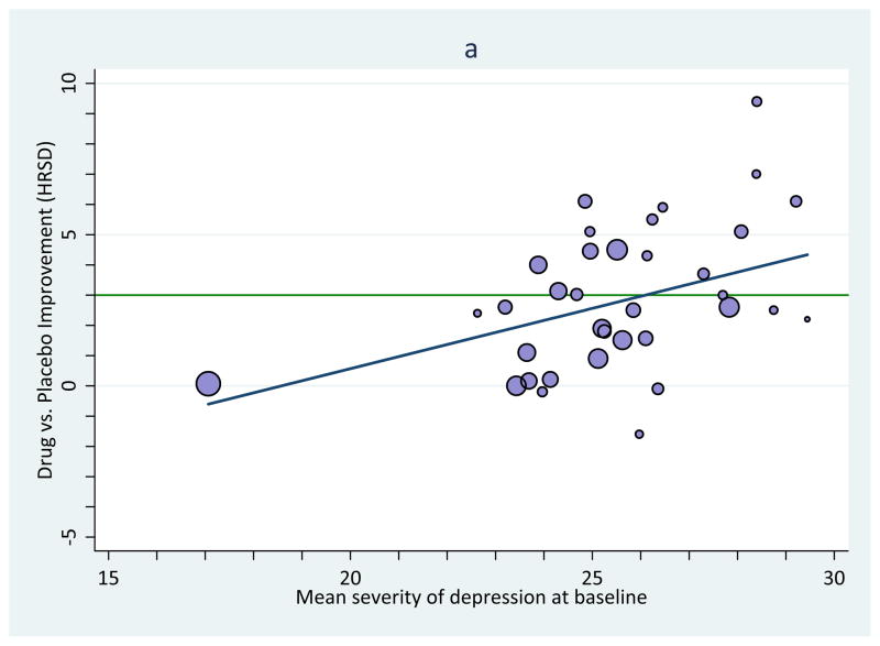
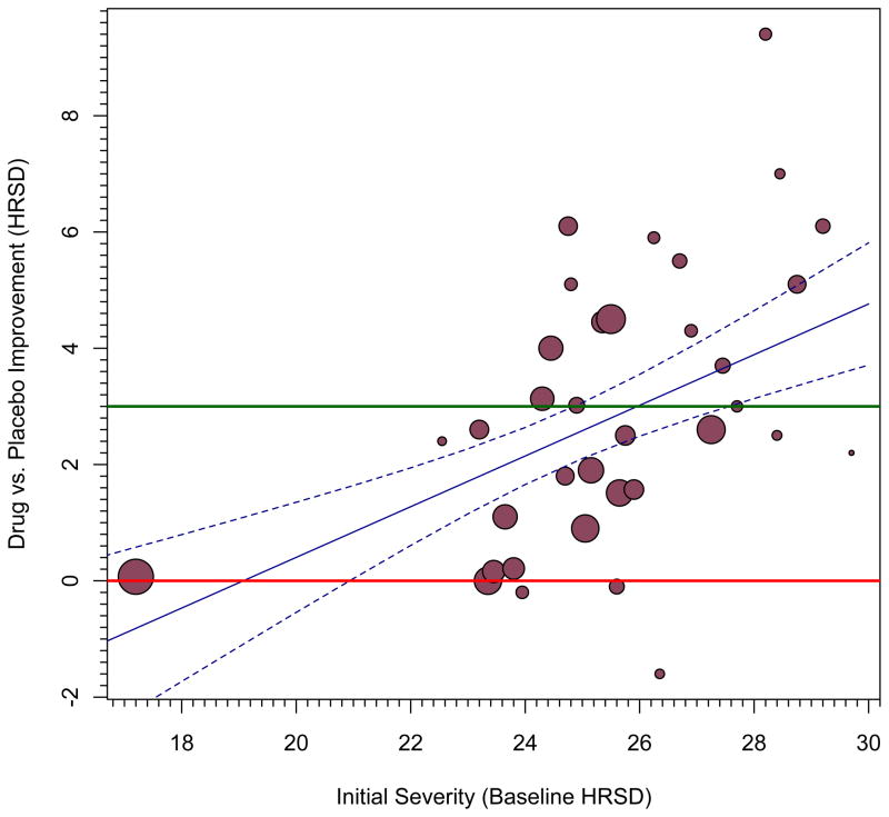
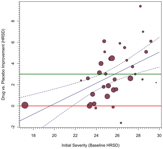
Results confirmed Kirsch and colleagues’ hypothesis: Antidepressant efficacy was indeed larger for samples with more extreme depression, Figure 1 (panel a) reprints their original graph of these findings; antidepressants’ efficacy did not reach a conventional value of clinical significance (green line) except in samples with very severe depression. Although such a display is useful for such purposes, a version with confidence bands would enable inferences not only about whether antidepressants have a statistically significant impact on depression (relative to placebo) but also, and more importantly, for samples with what levels of depression it has this effect. Unless otherwise noted, our demonstrations use point-wise confidence bands, which surround the meta-regression line, and point-wise confidence intervals, which are made at particular values of a moderator variable. (We address two other alternatives, simultaneous confidence bands and prediction bands, in the final section.)

Figure 1.

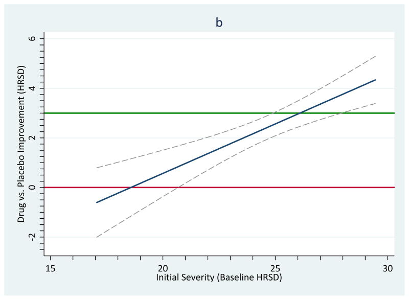
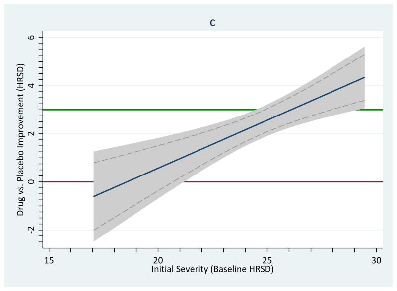
Improvement on depressive symptoms as a function of the samples’ baseline severity of depression generated using Stata commands; see text for more description.

Imagine that instead we want to know whether antidepressants have a statistically significant benefit for groups with an average level of depression of 17, the lowest value observed in any of the trials, which is in the “moderate” range of the scale. A starting point is the meta-regression equation of the line from their analysis:

$$\widehat{T}=-7.416+0.3991(\mathit{Baseline}\mathit{depression}),$$

where T̂ is the estimated value of the difference between drug and placebo improvement change. By default, meta-regression statistical output includes a test of whether the coefficient for the slope differs significantly from zero, which it was in this case, confirming Kirsch and colleagues’ prediction. (See Table 1, Model 1.) The slope shows that drugs had increasing success relative to placebo as the depression increased. Specifically, for every scale value worse on depression that a sample scored at baseline, the drug groups improved by 0.3991 HRSD scale points relative to placebo. Most meta-regression output includes estimates of the slope in two forms: (a) the unstandardized form, which we have described; and (b) the standardized form, usually characterized with the Greek symbol, β, which may be interpreted similarly to a correlation coefficient. In this case, the association between severity and the drug-placebo differences was β = 0.52.

Table 1.

Meta-regression equations of the line in which the constant is moved in order to estimate the difference in HRSD scale values for members of antidepressant groups relative to members of placebo groups for samples with varying levels of initial depression.

Model	Constant			Slope (95% CI)
	With HRSD value	T̂ (95% CI)	Width of CI
1	Original metric (constant=0)	−7.416 (−11.71, −3.12)	8.59	0.3991 (0.23, 0.57)
2	Original metric – 17	−0.630 (−2.04, 0.78)	2.82	0.3991 (0.23, 0.57)
3	Original metric – 20	0.567 (−0.37, 1.51)	1.88	0.3991 (0.23, 0.57)
4	Original metric – 23	1.765 (1.21, 2.32)	1.11	0.3991 (0.23, 0.57)
5	Original metric – 26	2.962 (2.43, 3.49)	1.06	0.3991 (0.23, 0.57)
6	Original metric – 29	4.159 (3.27, 5.05)	1.78	0.3991 (0.23, 0.57)
7	Original metric – 32	5.357 (4.00, 6.71)	2.71	0.3991 (0.23, 0.57)
8	Original metric – 46	10.940 (7.23, 14.66)	7.43	0.3991 (0.23, 0.57)

Note. The slope appears in order to help show that each model is estimating the same information. Rows that appear in yellow are extrapolations beyond the observed data. For simplicity, models follow fixed-effects assumptions; estimates incorporating random effects assumptions exhibited similar results. T̂=estimate of the degree of improvement in anti-depressant relative to placebo group members at the specified value of HRSD.

Although in practice many analysts might be satisfied to know the magnitude of the slope and its statistical significance, potentially even more useful is the intercept, which is the value that T̂ takes when the moderator variable (or variables) is (are) exactly zero. By default, meta-regression statistical output includes a test of whether the intercept differs significantly from zero, which it was in this case (T̂ = −7.416, 95% CI = −11.71, −3.12; Table 1, Model 1). In other words, we are 95% confident that the difference in improvement will be in the range from −11.71 to −3.12 for a sample with an initial mean HRSD value of 0.¹ Thus, if a sample’s mean baseline depression is exactly zero, this equation predicts that groups receiving placebo would average 7.416 HRSD scale points lower than groups receiving antidepressants. This example helps to illustrate one reason why meta-regression intercepts are so commonly ignored in practice—because they so often yield unrealistic values. In this particular case, the intercept reflects a value that baseline HRSD means cannot plausibly take. Although it is possible for an individual to score 0 on the HRSD, a sample could not have a mean score of exactly 0 unless it also had zero variance as well, which would be a rare occurrence indeed. Moreover, when depression levels are so low, there is no need for anti-depressants, let alone in predicting what their effects would be.² Much more valuable is to see what impact drugs might have on populations with a real need for them. Finally, another reason to mistrust this estimate is that there were no observations so low in the database and therefore the estimate is a fairly extreme extrapolation.

Imagine that we want to know what impact anti-depressants should have on patients whose level of depression is HRSD=17, which is the lowest value observed in this particular sample of studies and is conventionally interpreted as a moderate depression. Inserting this value into the equation of the line yields:

$$\widehat{T}=-7.416+0.3991(17)=-\mathrm{0.6313.}$$

In other words, the equation predicts that members of the drug group will improve less (by 0.6313 HRSD scale values) than members of the placebo group. Although it is simple to determine a predicted value using the equation of the line, in order to create a confidence interval around it, one must use the moving constant technique.³ Specifically, subtracting 17 from every observation of baseline severity will effectively move the intercept to a value of 17. Now when we re-run the model, the results show not only the same estimated value of T̂ the equation implied, −0.630, but also a confidence interval for it (−2.04, 0.78), as Model 2 in Table 1 shows. Thus, for samples with moderate levels of depression, no advantage is likely to be seen for those taking antidepressants (relative to those taking placebo). Note that the confidence interval around this value is also much narrower, which makes sense because there are some data available at this point along the moderator variable to create an estimate (see Figure 1, panel a).⁴

Table 1 uses the same procedure to estimate other confidence intervals across the observed range of the moderator variable. A significant effect of drug is evident when the mean HRSD scale value reaches 23 (model 4), and the drug effect continues to increase and be statistically significant at higher HRSD scale values. Another important benchmark is clinical significance: An effect might be statistically significant without having sufficient practical impact in people’s lives. In the present case, Kirsch et al. (2008) noted that the 3-point NICE clinical significance benchmark was achieved somewhere near the 28-point mark of the moderator variable. Indeed, at the highest observed initial depression value, 29 (model 6), the confidence interval no longer includes 3. Thus, on the average for studies whose samples had mean levels of initial depression this high, the observed values exceeded the clinical significance criterion.

For the purpose of illustration, we estimated two more models that move beyond the observed range of the moderator variable. Just as the confidence interval for a sample with zero depression had a wide range, so too does the confidence interval for a sample of extremely depressed patients (46 on the HRSD scale), in model 8. These extreme examples might strike some readers as controversial: Conventionally, statisticians restrict estimates to observed ranges of moderator variables, but there are times when it is important to project findings beyond what was observed, such as when earth scientists project climate change over centuries. As an example, earth scientists commonly project estimates far into the future, such as how much the earth will warm by the year 2100 and even centuries farther into the future (Solomon et al., 2009), or how high the seas will rise given this amount of warming. Obviously, such predictions can have profound ramifications. Having some confidence in how conditions may change can help community planners protect their territories and maximize outcomes. ⁵

The above models imply how one can estimate confidence bands around the predicted values defined by T̂s. Such is the logic of regression, whether in terms of regular regression with primary-level data (e.g., Myers and Well, 2003) or with meta-analytic data (Viechtbauer, 2010a). One can move the intercept across the values of a moderator and plot the estimate and its confidence interval. The problem with moving it in such a coarse fashion is that, if the points estimated are very distant from each other, a graph based on this procedure may have poor smoothing between the estimates and might badly estimate certain regions along the moderator variable. Greater accuracy would result if the estimates moved in much finer increments along the moderator variable. In the current example, 1,001 iterations that each move the intercept by 0.0123809 of a unit of depression creates an extremely precise estimate of the confidence bands. If we start with mean depression at its minimum observed value, 17.0631, then after 1,001 iterations, the intercept would estimate the maximum observed depression in these samples, 29.444, and the resulting confidence bands will be smoother. Of course, such fine gradations might not be necessary unless a very high resolution graph is needed, such as when it will be printed in a very large size. Our Appendixes list syntax to show how one can create such graphs using two popular statistical platforms and Figure 1, panel b, shows such a graph. A significant difference exists when the confidence bands no longer include the red line indicating exactly no difference. A clinically significant difference exists when the confidence bands exceed the green reference line.

As we have illustrated, the moving constant strategy is also helpful for producing point estimates at points of interest, with no graphs at all. To examine estimates along a continuous moderator variable that is examined linearly, one would typically plot estimates for the lowest and highest value observed for the moderator variable. Plotting estimates at the mean or median values of the moderator might also be of interest, and other possibilities may exist as well, such as projecting results beyond the observed range of the moderator variable. Thus, an analyst could plot T̂ at specified points along the continuum implied by the moderator variable and report the estimated weighted T̂ and the confidence interval around this estimate.

Potential problems with bands produced by graphing functions in conventional software

Because they are easily invoked, one temptation might be to graph such patterns with conventional, widely-available software that was written for use with primary-level data and includes ordinary weighted least squares analysis functions. For example, one can use SPSS (IBM SPSS Statistics, 2010) to plot confidence bands around weighted regression lines, but because the graphing solution models the standard error of the regression coefficients (including the intercept) differently than conventional meta-analytic statistics in relation to their unstandardized coefficients, β̂_j, the confidence bands and intervals will almost always differ from those implied by the meta-analytic regression (see Lipsey & Wilson, 2001, pp. 138–140). Hedges and Olkin (1985) noted that “standard errors for β̂_j printed by the program are incorrect by a factor of $\sqrt{{MS}_E}$, where MS_E is the error or residual mean square for the regression” (p. 174, italics in original) because standard software does not incorporate the known variance estimate for the meta-analytic data (Konstantopoulos and Hedges, 2004).⁶ Although Hedges and Olkin made their statement in reference to fixed-effects meta-regression models, models that incorporate random-effects assumptions are just as susceptible to the problem.⁷ Future research should address this issue.

In order to keep graphical depictions of meta-analytic results squarely in accord with the underlying inferential statistics, therefore, analysts are well advised to avoid using standard software for graphing meta-regression results, or at least to double-check that the confidence bands match the meta-analytic model. The logic we outlined in this section can be used for such a check: Estimate the confidence intervals for a value along the moderator dimension in question and compare them to the figure. In Figure 1, panel c, the dashed lines indicate the confidence bands implied by a meta-regression following mixed-effects assumptions; grey bands resulted by invoking the weighted graphing function in primary-level statistical software (i.e., using the Stata command twoway lfitci). These bands (shaded area) are clearly wider; thus, statistical and clinical inference will deviate at certain points along the moderator.

Importantly, ordinary weighted least squares analyses do not always overestimate the widths of confidence bands: In fact, the difference can go in either direction. As Hedges and Olkin, above, implied, the bias is more conservative (wider confidence intervals and bands) to the extent that $\sqrt{{MS}_E}$ exceeds 1, more liberal (narrower intervals and bands) to the extent that $\sqrt{{MS}_E}$ is less than 1, and equivalent when $\sqrt{{MS}_E}=1$. Consequently, using ordinary weighted least squares analysis functions to estimate confidence intervals and bands will be justified only in the very rare instance when $\sqrt{{MS}_E}=1$.

The Moving Constant Technique in More Complex Meta-Regression Models

Multiple-moderator models

To this point, we’ve used a bivariate meta-regression example to make use of the intercept completely transparent. Now we turn to a more complicated example that better maps on to the target problem. Assume we have a meta-analysis of studies using exercise to impact quality of life in cancer survivors, such as Ferrer and colleagues (Ferrer et al., 2010) recently conducted. Imagine that we want to illustrate a model with three moderator variables that we find plausible based on a reading of the literature: (a) the quantity of aerobic METs; (b) its quadratic term (i.e., aerobic METs²); and (c) the percentage of the sample that is female. Aerobic METs are literally “metabolic equivalents of task,” which define how active one is. At rest, one exerts 1 MET; at 6 METs one does vigorous exercise. The studies evaluate the extent to which bouts of exercise that accrue over time relate to quality of life assessed on standard scales.

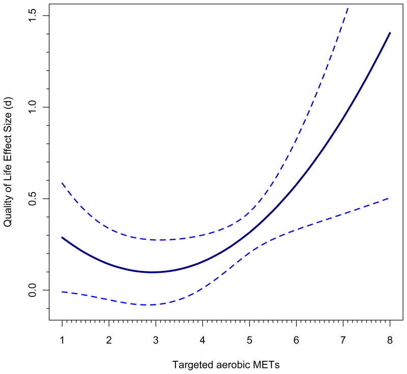
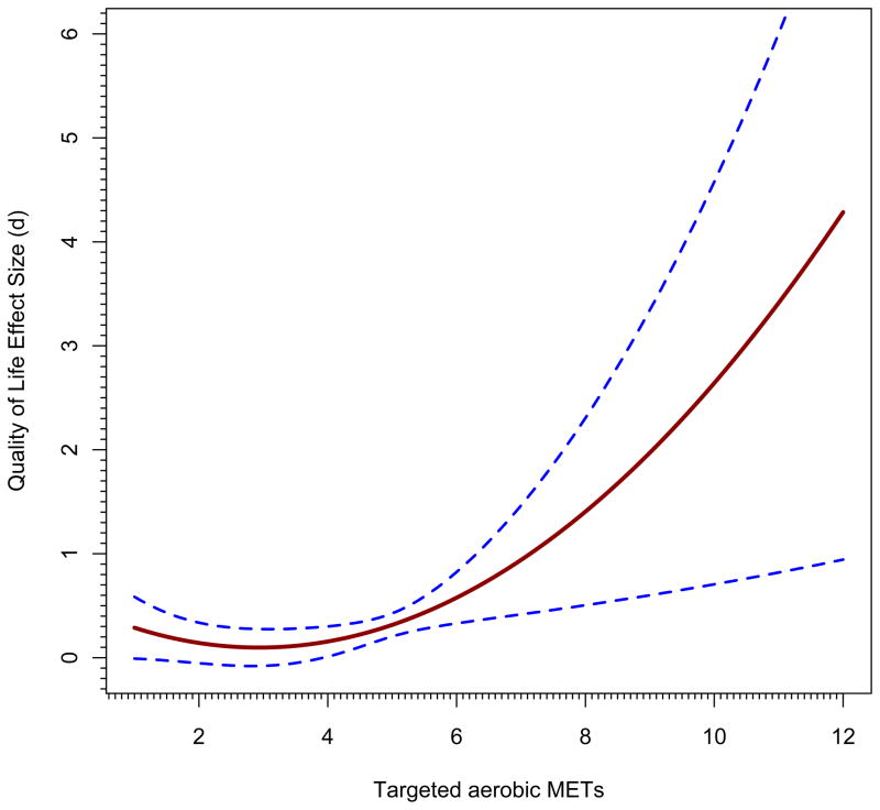
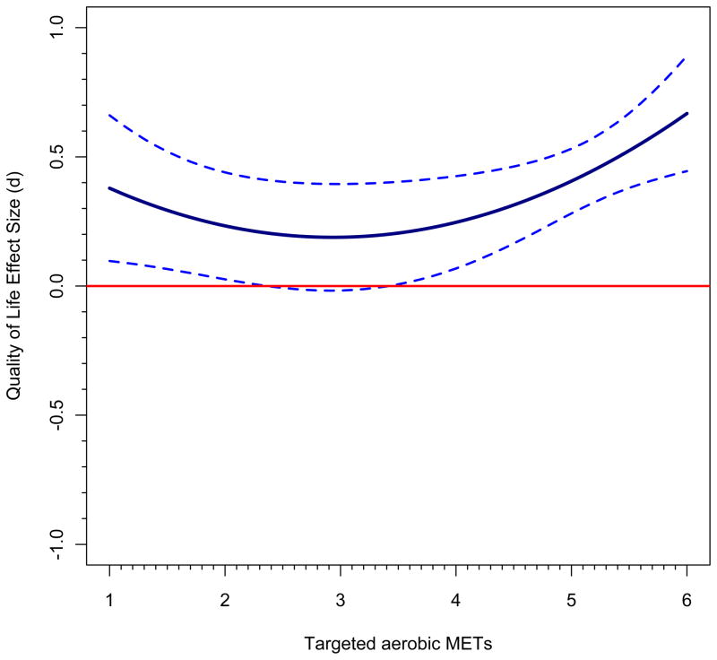
Just as in ordinary regression, a model with quadratic effects must incorporate the linear effect because otherwise a statistically significant quadratic effect might in reality be a linear effect. First, let’s examine trends across the range of aerobic METs, holding the impact of sample gender constant at its sample mean of 79% female; thus, gender is zero-centered at 79% in this analysis. Although all-male and all-female samples appeared in the database, more female than male samples were present. Figure 2, panel a, shows the first figure that results from following these steps (see Appendix I). We see that the impact of exercise is statistically significant across the range from medium (4 MET) to very high (8 METs) targeted aerobic activity. No study had a value over 6.25 METs, so after that point, as discussed above, any regression line and confidence bands beyond this point amount to a prediction of what would happen at these higher activity points. Panel b takes it to greater extremes, but indicates where no underlying observations exist by changing the line to be dotted at the 6.25 value; still, it projects estimates all the way to aerobic METs=12, far higher than any study evaluated. First note that although the confidence bands in this graph in the portion of the graph up to METs=8 appear to be narrower, they are in fact the same; it is just that the maximum value of the Y-axis is now much larger, to SMD=6. Nonetheless, one can see that the CIs widen dramatically, just as they should, because there are no observations in that region. The figure is also quite implausible from the standpoint that the largest observed effect size is less than SMD=2 and the predicted values plotted go far beyond this value. Such a figure predicts what might happen if cancer survivors were given extremely strenuous aerobic activities and if they could undertake such a program. An analyst might use a figure such as this one if he or she was trying to encourage scholars to undertake such trials and to see whether still greater improvements in quality of life can occur.

Figure 2.

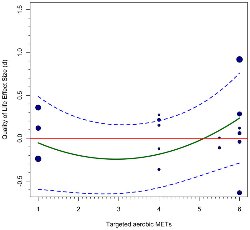
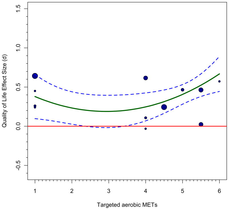
Complex meta-analytic models plotted under differing circumstances implied by the models. Specifically plotted is the relation between intensity of aerobic exercise on quality of life improvements for cancer survivors. See text for more description.

It is important to understand that, because gender was zero-centered in these models, strictly speaking, graphs such as Figure 2’s Panels a and b plot the estimated improvement of various amounts of aerobic exercise, adjusted so that they reflect samples with 79% females (the mean). Our model showed that samples with larger percentage of females had greater success improving quality of life through exercise. Thus, the plotted line is logically farther from zero for samples that are more female and closer to the line for samples that are more male. The same sequence that produced Figure 2, panel a, was followed for these two extremes. In two new instantiations, we hold gender constant at 0 or 100%, respectively. Panels c and d show the estimates for samples of males and females, respectively. Although both lines show the curvilinearity implied by the quadratic function, the line is indeed farther from zero for female samples and closer to zero for male samples. Indeed, aerobic exercise would appear to have little impact on quality of life for samples of males unless more intense aerobic exercise is undertaken and then just barely. For female samples, in contrast, any amount of exercise appears to improve quality of life, but especially at higher intensities. Note too that the confidence bands are narrower for female than for male samples, consistent with the fact that there were more observations for the former group. As with any meta-analytic model, the analyst should take care to note such limitations when interpreting such findings. The authors of this particular meta-analysis used exactly these procedures to evaluate more sophisticated models of the relation, showing that the quadratic function did not appear unless the patients exercised steadily over a few months; interested readers should consult their article (Ferrer et al., 2010), which lists other limitations of this particular meta-analysis.

Complications involving categorical variables

Up until this point, our examples of used continuous variables as moderators. Note that the moving constant technique can help an analyst avoid the problem of bifurcating continuous variables; that is, the models themselves can produce estimates for particular levels of the continuous variables, obviating the need to artificially dichotomize them. Yet, categorical variables commonly occur in meta-analytic research and they present some special complications. Imagine we are still pursuing the same meta-analytic model as in the preceding paragraphs, but that now gender is represented as two categories, male and female, instead of as a continuous variable, percentage of females in the sample. Orthogonal coding gender so that male samples are −1 and female samples are +1 effectively controls the gender effect when estimating other moderators’ effects. Now, interpretation proceeds as we have already described.

Imagine further what the results would imply if one instead dummy-coded the sample gender variable so that male samples are 0s and female samples are 1s, leaving aerobic METs (and its quadratic function) in the original metric. Now the intercept in the model would reflect the point at which the moderator variables are all 0, that is, male samples with aerobic METs=0. Once again, we find ourselves backed into a statistical corner where the intercept has little or no meaning because the METs scale begins not at value 0 but at 1, which implies being at rest. The solution of course, is to commence with the intercept of our model reflecting the lowest value of the scale (1) rather than the meaningless value of 0. Finally, complexities in such models increase as the numbers of moderator variables increase, but the underlying logic to display the results is the same as we have presented here. For example, Johnson and colleagues (Johnson et al., 2003) fit a meta-regression model with 5 moderators in their meta-analysis of studies evaluating HIV prevention interventions for adolescents. Three variables were continuous and two were categorical (dummy coded). It took them 14 meta-regression runs to produce estimates for the extremes of each moderator while statistically holding the other moderators’ influences constant at zero.

Is zero-centering or contrast-coding moderators always the best solution?

Some readers may take the preceding examples to imply that one must zero-center or contrast code all moderators except for the one that is the focus of the moving constant technique in order to portray estimates and their confidence intervals or bands across that moderator. Yet, especially when interactions between moderators exist, it may be preferable to produce estimates that follow differing assumptions. Imagine, as is often the case, that the studies in a particular meta-analysis vary in methodological quality. Suppose we are examining the effects of exercise on depression levels in cancer survivors and expect to see a dose-response curve such that depression improves with greater amounts of exercise. An analyst could regress Ts on exercise dose, study quality, and the interaction of these terms. (Note that the analysis to examine the statistical significance of these terms will likely be more stable if the dose and quality terms are zero-centered before multiplying them to create the interaction term.) Suppose further that the interaction is statistically significant. In such a circumstance an analyst might well show the dose-response pattern with study quality held constant at a high level because, logically, these are the studies whose results are the most trusted. Alternatively, one might show the dose-response function for both high- and low-quality studies. Brown and colleagues (Brown et al., 2011) followed just these procedures in their meta-analysis examining the effects of resistance exercise on cancer-related fatigue (see their Table 4). A dose-response pattern was most marked for the highest quality studies.

Caveats about clinical significance

Because no standard for clinical significance yet exists for quality of life outcomes, we have focused instead on statistical significance in this section. The fact that there are many different scales to assess quality of life makes achieving clinical significance standard more difficult, but not impossible. Indeed, if one wished to parallel the NICE criterion for depression change, one could generalize from the fact that their clinical significance criterion specifies the target of a “medium” effect size of SMD=0.50, per Cohen’s (1988) standards. Consequently, a medium effect size implies a change that is visible to the naked eye, with no need for statistics (Johnson and Kirsch, 2008). The graphs in Figure 2 might be interpreted as failing to meet this clinical significance standard, as none of the confidence bands exceed this value.

General Limitations and Potential Uses of These Strategies

It is worth discussing some other potential uses of the strategies we have described as well as some general limitations, including assumptions that underlie the statistical model, detecting outliers, using prediction intervals, producing Bayesian estimates, strategies for alternative confidence bands, and practical limitations.

Assumptions underlying the model

Sources on meta-analysis routinely state how, under heterogeneity, fixed-effects assumptions typically produce overly-narrow confidence intervals relative to random- and mixed-effects assumptions. To illustrate, Figure 3 portrays the same antidepressant data that appeared in Figure 1. Panel a follows fixed-effects assumptions and Panel b follows random-effects assumptions. Because heterogeneity is present, in a formal sense the fixed-effects version is incorrectly specified; consequently, it has overly liberal, narrower confidence bands (panel a) and the random-effects version with its wider confidence bands might instead be favored (panel b). In this case, statistical inference does not dramatically differ between the two sets of estimates. It should also be noted that the variables that enter into the statistics themselves may be subject to any number of problems, including non-normal sampling distributions, invalidity, unreliability, and restriction of range, to name only a few (Hunter and Schmidt, 2004; Cohen et al., 2004).

Figure 3.

Improvement on depressive symptoms as a function of baseline severity of depression, with each point sized proportionally to its weight in the analysis. Panel a: Moderation pattern showing regression line and 95% confidence band under fixed-effects assumptions. Panel b: Same as Panel b but under mixed-effects assumptions (i.e., with a random-effects constant and a fixed-effects slope).

Outlier detection

Graphs such as we have produced can be helpful in diagnosing problems in the literature; we implied just this function at the outset, in discussing bivariate meta-regressions. The same holds for the more complex examples we presented in the preceding section. It is most valuable to use the more complex patterns implied by the model, thus we can understand the influence of some particular relevant moderators while controlling for the effect of others. Panels e and f of Figure 2 use the regression lines and confidence bands from panels c and d because these represent the complete model that was evaluated; superimposing observed effect sizes on the overall model, zero-centering gender, would be prone to error because it does not account for the gender effect. If we still did so, relatively large effect sizes would be more likely to be from studies that focused on females and relatively small (or negative) effect sizes would be more likely to have focused on males. The fact that sample gender is represented in continuous form whereas our graphs focus on the extremes of the distribution created a problem, because we had to pick which effect sizes to plot in each graph. It seems reasonable to plot cases with 50% or more males in the former plot and those with 50% or more females in the latter plot. One can see that the regression lines stay closer to studies with larger weights, which illustrates meta-analytic weighting in action. These plots also visually show residuals, which is the difference between the estimated value and the observed value for each case. Those farther from their lines have larger residuals. There are indeed far fewer cases for male cancer survivors, so statistical inferences are quite strained here. Both panels show that there are few studies in the range under METs=4, again implying that predictions here are a projection. The quadratic function appears most justifiable for the female sample studies, although there are some outliers that would be worth inspecting. Alternatively, other moderators might improve prediction and eliminate these large residuals.

Prediction intervals

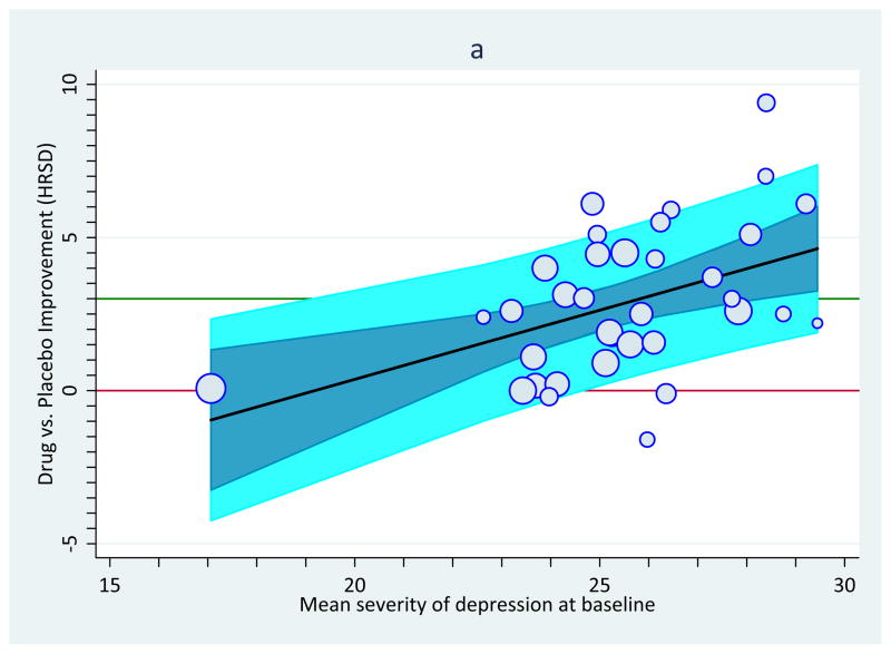
This article focused most on estimating Ts at certain points along a moderator dimension or dimensions, which boils down to estimating where the weighted mean T lies along a moderator or set of moderators. Another alternative is to portray the prediction interval in which future studies are likely to be observed in relation to a moderator dimension or dimensions. As Borenstein and colleagues discuss and illustrate with a worked example, this strategy addresses the dispersion of effect sizes that one is likely to see in a particular literature. Our Appendix I lists steps that can be used in one statistical platform to produce such estimates in tandem with meta-regression models. Figure 4, panel a shows a graph with such estimates for the Kirsch anti-depressants data, showing that the prediction interval is much wider than the confidence bands. An analyst might display such a graph in order to develop expectations for how large T will be in a new study that matches a particular level of a moderator variable or variables, making it an adjunct to power analysis strategies.

Figure 4.

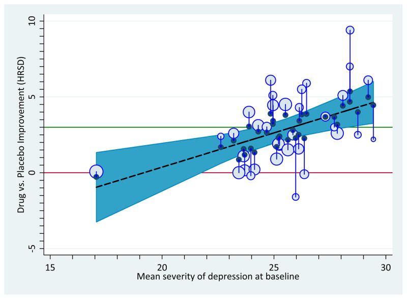
Improvement on depressive symptoms as a function of baseline severity of depression, with each point sized proportionally to its weight in the analysis, and following mixed-effects assumptions. Panel a: Moderation pattern showing 95% prediction intervals. Panel b: Observed (open circles) and empirical Bayesian estimates (filled circles) of true effect sizes.

Bayesian estimates

The solutions that we described in the preceding two sections are decidedly frequentist in orientation, a practice often labeled classical meta-analysis. Nonetheless, those who wish to construct similar graphs following Bayesian assumptions can do so. In Figure 4, panel b, we portray the empirical Bayesian estimates of the true effects for each study (once again in the Kirsch antidepressants database), assuming the fitted model is correct (see Appendix I). In this graph, the observed SMDs appear as bubbles and the adjusted, true SMDs appear as filled bubbles. Arrows show how the observed SMDs converge on the regression line of the meta-regression model in the empirical Bayesian estimates of the true SMDs. Those cases that before appeared to be outliers as observed appear much more consistent under the assumptions of this model.

Simultaneous confidence bands

The strategy that we have emphasized in this article is the point-wise method of constructing confidence bands and intervals. The simultaneous confidence band strategy attempts to control for the expanded error rate that accrues from the evaluating a statistical hypothesis across the range of a moderator variable or variables (Liu et al., 2008; Seber and Lee, 2003; Working and Hotelling, 1929). The point-wise strategy we have illustrated in this article would presumably suffer from heightened Type-I error rates, stemming from examining whether T̂ is significant at different levels of a moderator variable or variables. Note that, in theory, a moderator dimension can be divided into infinite increments and heightening Type-I (α) rates. The Bonferroni correction is often applied to reduce Type-I error rates by dividing α by the number of tests being evaluated, but cannot be invoked when there is an infinity of tests. This impasse, coupled with the lack of a priori conceptualization for critical values of the moderator variables in models, suggests that analysts should routinely set α to be more stringent to compensate or else interpret results more conservatively. Importantly, to date, there appears to be no easily available strategy for applying the simultaneous confidence band solution in meta-regression. Future research should address these problems directly.

Practical limitations

It is worth discussing when graphs such as we have produced here might be most valuable. Given that most meta-analyses investigate numerous moderator variables, plotting all patterns might often prove impractical. If the goal is comprehensiveness, then tables of output are much more compact than numerous figures. Instead, the patterns that deserve the most practical attention are the ones that analysts should graph, the ones that they want to help tell the story of their meta-analytic results. Finally, it is worth noting that successful graphing is often an intensive, iterative practice in which the analyst produces successive versions of the same pattern until the right combination of informativeness and aesthetic value is achieved (Tufte, 2001).

One potential limitation of the steps we have listed here to depict meta-regression results is financial. True, some of our graphs were created using the commercial software Stata (Stata Corp, 2009) (see Appendix I). The Lipsey and Wilson (2001) macros also are available for SPSS and SAS, both also commercial.⁸ Those who are students rather than professionals often can get discounted prices on such software. Fortunately, all or nearly all of the solutions we suggest are also available in the open-access statistical software R (see Burns, 2006), for which Viechtbauer (Viechtbauer, 2010a; Viechtbauer, 2010b) has written a sophisticated suite of meta-analysis protocols, metafor. Appendix II shows how we used this software to create graphs such as in Figure 2 and panels a and b of Figure 3.

Conclusion

Several prominent sources have given careful attention to graphing primary-level data and offer sage advice that meta-analysts might well also incorporate. Specifically, Tufte (Tufte, 2001; Tufte, 2006) argued for more careful integration of graphical and textual information, much in the way in which Leonard da Vinci’s journals illustrate. Research has shown that the modern practice of separating text and graphics yields poorer communication of the targeted scientific information (Sweller et al., 1990). Two other sources provide very helpful advice about how best to represent more nuanced aspects of scientific databases (Cleveland, 1984; Lane and Sandor, 2009). To date, such sources emphasize primary-level investigations almost entirely to the exclusion of meta-analysis. The current article has emphasized how many of these principles of effective graphical displays generalize particularly well to effect size information. In sum, the strategies we have described here should enable meta-analysts to create accurate graphs of meta-regression results and more effectively communicate scientific information. Because graphical depictions of statistical results are often a highly desirable way to “tell the story” related to a given phenomenon, strategies such as we have detailed should be an indispensible tool in meta-analysts’ toolkit.

References

- Berkey C, Hoaglin DC, Mosteller F, Colditz GA. A random-effects regression model for Meta-analysis. Stat Med. 1995;14:395–411. doi: 10.1002/sim.4780140406. [DOI] [PubMed] [Google Scholar]
- Borenstein M, Hedges LV, Higgins JPT, Rothstein HR. Introduction to Meta-analysis. John Wiley & Sons; West Sussex: 2009. [Google Scholar]
- Borman G, Grigg JA. Visual and narrative interpretation. In: Cooper H, Hedges LV, Valentine JC, editors. The Handbook of Research Synthesis and Meta-analysis. 2nd Ed. Russell Sage Foundation; New York: 2009. pp. 497–519. [Google Scholar]
- Brown J, Huedo-Medina TB, Pescatello LS, Pescatello SM, Ferrer RA, Johnson BT. Efficacy of exercise interventions in modulating cancer-related fatigue among adult cancer survivors: A meta-analysis. Cancer Epidem Biomar. 2011;20:123. doi: 10.1158/1055-9965.EPI-10-0988. [DOI] [PubMed] [Google Scholar]
- Burns P. [Accessed 10 June 2010];R relative to statistical packages: A look at Stata, SAS and SPSS. 2006 ( http://lib.stat.cmu.edu/S/Spoetry/Tutor/R_relative_statpack.pdf)
- Cleveland W. Graphs in Scientific Publications. Am Stat. 1984;38:261–269. [Google Scholar]
- Cohen J. Statistical power analysis for the behavioral sciences. 2nd Ed. Lawrence Erlbaum Associates; 1988. [Google Scholar]
- Cohen P, Cohen J, Aiken LS, West SG. The problem of units and the circumstance for POMP. Multivar Behav Res. 1999;34:315. [Google Scholar]
- Cooper H, Hedges LV, Valentine JC. The Handbook of Research Synthesis and Meta-analysis. 2nd Ed. Russell Sage Foundation; New York: 2010. [Google Scholar]
- Ferrer R, Huedo-Medina TB, Johnson BT, Stacey R, Pescatello L. Exercise interventions for cancer survivors: A Meta-analysis of quality of life outcomes. Ann Behav Med. 2010;41:32–47. doi: 10.1007/s12160-010-9225-1. [DOI] [PMC free article] [PubMed] [Google Scholar]
- Harbord R, Higgins JPT. Meta-regression in Stata. The Stata J. 2008;8:493–519. [Google Scholar]
- Hayter A, Liu W, Wynn HP. Easy-to-construct confidence bands for comparing two simple linear regression lines. J Stat Plann Infer. 2007;137:1213–1225. [Google Scholar]
- Hedges L. Meta-analysis. J Educ Stat. 1992;17:279–296. [Google Scholar]
- Hedges L, Olkin I. Stastical Methods for Meta-analysis. Academic Press; Orlando: 1985. [Google Scholar]
- Hedges L, Vevea JL. Fixed- and random-effects models in meta-analysis. Psychol Meth. 1998;3:486–504. [Google Scholar]
- Higgins J, Green S. [Accessed 18 February 2011];Cochrane Handbook for Systematic Reviews of Interventions, Version 5.0.2. 2009 ( www.cochrane-handbook.org)
- Higgins J, Thompson SG. Quantifying heterogeneity in a meta-analysis. Stat Med. 2002;21:1539–58. doi: 10.1002/sim.1186. [DOI] [PubMed] [Google Scholar]
- Huedo-Medina T, Johnson BT. Netbiblio, La Coruña. 2010. Modelos Estadísticos en Meta-análisis [Statistical Models in Meta-analysis] [Google Scholar]
- Hunter J, Schmidt FL. Methods of meta-analysis: Correcting error and bias in research findings. 2nd Ed. Sage Publications; Thousand Oaks: 2004. [Google Scholar]
- IBM. SPSS Statistics. SPSS Inc; Chicago: 2010. Release 19.0. [Google Scholar]
- Johnson BT, Carey MP, Marsh KL, Levin KD, Scott-Sheldon LAJ. Interventions to reduce sexual risk for the human immunodeficiency virus in adolescents, 1985–2000. Arch Pediatr Adol Med. 2003;157:381–388. doi: 10.1001/archpedi.157.4.381. [DOI] [PubMed] [Google Scholar]
- Johnson BT, Kirsch I. Do antidepressants work? Statistical significance versus clinical benefits. Significance. 2008;5:54–58. [Google Scholar]
- Kirsch I, Deacon BJ, Huedo-Medina TB, Scoboria A, Moore TJ, Johnson BT. Initial severity and antidepressant benefits: A meta-analysis of data submitted to the Food and Drug Administration. PLoS Med. 2008;5:e45. doi: 10.1371/journal.pmed.0050045. [DOI] [PMC free article] [PubMed] [Google Scholar]
- Knapp G, Hartun J. Improved tests for a random-effects meta-regression with a single covariate. Stat Med. 2003;22:2693–2710. doi: 10.1002/sim.1482. [DOI] [PubMed] [Google Scholar]
- Konstantopoulos S, Hedges LV. Meta-analysis. In: Kaplan M, editor. The Handbook of Quantitative Methods in the Social Sciences. Sage Publications; Thousand Oaks: 2004. pp. 281–297. [Google Scholar]
- Konstantopoulos S, Hedges LV. Analyzing effect sizes: Fixed-effects models. In: Cooper H, Hedges LV, Valentine JC, editors. The Handbook of Research Synthesis and Meta-Analysis. 2nd Ed. Russell Sage Foundation; New York: 2009. pp. 279–294. [Google Scholar]
- Lane D, Sándor A. Designing better graphs by including distributional information and integrating words, numbers, and images. Psychol Meth. 2009;14:239–257. doi: 10.1037/a0016620. [DOI] [PubMed] [Google Scholar]
- Lau J, Ioannidis JPA, Terrin N, Schmid CH, Olkin I. The case of the misleading funnel plot. Br Med J. 2006;333:597–600. doi: 10.1136/bmj.333.7568.597. [DOI] [PMC free article] [PubMed] [Google Scholar]
- Light E, Singer JD, Willett JB. The visual presentation and interpretation of meta-analyses. In: Cooper H, Hedges LV, Valentine JC, editors. The Handbook of Research Synthesis and Meta-analysis. 2nd Ed. Russell Sage Foundation; New York: 1994. pp. 439–453. [Google Scholar]
- Lipsey M, Wilson DB. Practical Meta-Analysis. Sage Publications; Thousand Oaks: 2001. [Google Scholar]
- Liu W, Lin S, Piegorsch WW. Construction of exact simultaneous confidence bands for a simple linear regression model. Int Stat Rev. 2008;76:39–57. [Google Scholar]
- Myers J, Well AD. Research Design and Statistical Analysis. Lawrence Erlbaum; Mahwah: 2003. [Google Scholar]
- Raudenbush S. Analyzing effect sizes: Random-effects models. In: Cooper H, Hedges LV, Valentine JC, editors. The Handbook of Research Synthesis and Meta-Analysis. 2nd Ed. Russell Sage Foundation; New York: 2009. pp. 295–315. [Google Scholar]
- Seber G, Lee AJ. Linear Regression Analysis. 2nd Ed. John Wiley & Sons; New Jersey: 2003. [Google Scholar]
- Solomon S, Plattner G, Knutti R, Friedlingstein P. Irreversible climate change due to carbon dioxide emissions. P Natl Acad Sci USA. 2009;106:1704. doi: 10.1073/pnas.0812721106. [DOI] [PMC free article] [PubMed] [Google Scholar]
- StataCorp. Stata Statistical Software: Release 11. StataCorp LP; College Station: 2009. [Google Scholar]
- Sweller J, Chandler P, Tierney P, Cooper M. Cognitive load as a factor in the structure of technical material. J Exp Psychol. 1990;119:176–192. [Google Scholar]
- Tufte E. Beautiful Evidence. Graphic Press; Cheshire: 2006. [Google Scholar]
- Tufte E. The Visual Display of Quatitative Information. 2nd Ed. Graphic Press; Cheshire: 2001. [Google Scholar]
- Viechtbauer W. [Accessed 10 June 2010];The metafor Package: A Meta-analysis package for R. 2010a ( http://www.wvbauer.com/downloads.html)
- Viechtbauer W. Conducting Meta-analyses in R with the metafor package. J Stat Software. 2010b;36:1–48. [Google Scholar]
- Working H, Hotelling H. Applications of the theory of error to the interpretation of trends. J Am Stat Assoc. 1929;24:73–85. [Google Scholar]
Associated Data
This section collects any data citations, data availability statements, or supplementary materials included in this article.