Biologically inspired intelligent decision making

Abstract

Artificial neural networks (ANNs) are a class of powerful machine learning models for classification and function approximation which have analogs in nature. An ANN learns to map stimuli to responses through repeated evaluation of exemplars of the mapping. This learning approach results in networks which are recognized for their noise tolerance and ability to generalize meaningful responses for novel stimuli. It is these properties of ANNs which make them appealing for applications to bioinformatics problems where interpretation of data may not always be obvious, and where the domain knowledge required for deductive techniques is incomplete or can cause a combinatorial explosion of rules. In this paper, we provide an introduction to artificial neural network theory and review some interesting recent applications to bioinformatics problems.

Introduction

Artificial neural networks (ANNs) are statistical machine learning models which emulate the processing technique of biological neurons to perform function approximation and pattern recognition from a set of exemplars, in a way which can generalize its mapping to new data.^1-3 ANNs are finding use across a number of domains for classification^4-7 and function approximation.^8-10 Figure 1, which plots number of bioinformatics papers in PubMed^11,12 that reference neural networks over the period 1994 to 2009, suggests that there is an increasing trend in the application of ANNs to bioinformatics problems.¹³

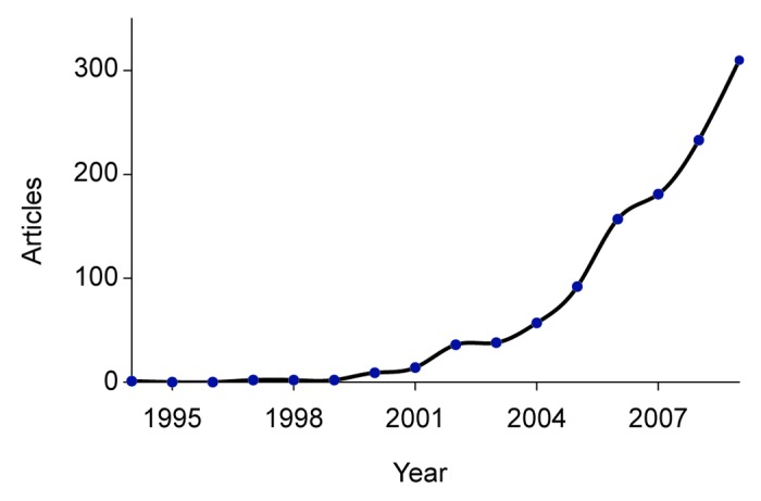
Figure 1. The number of bioinformatics papers in PubMed that reference neural networks, grouped by year.

This paper begins with an introduction to neural networks, providing a description of what they are and how they are used, as well as a high level description of how they work. The advantages and disadvantages of ANNs are discussed, and information considered pertinent to their practical application is presented by way of a number of examples.

Further analysis of the literature available on PubMed, as shown in Figure 2, indicates that the 3 main bioinformatics topics which reference neural networks are:

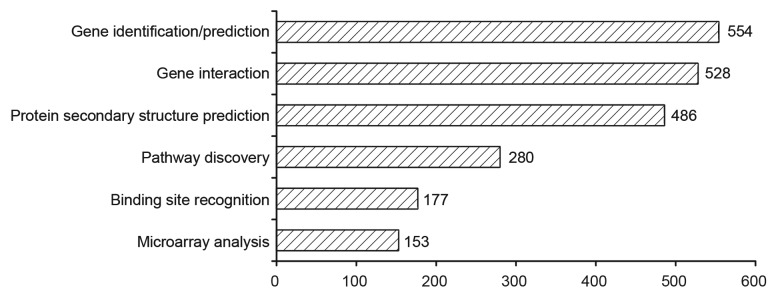
Figure 2. Breakdown of bioinformatics topics identified across a number of analyzed papers available on PubMed which reference neural networks.

• Gene identification/prediction (554 papers)

• Protein secondary structure prediction (486 papers)

• Gene interaction (528 papers)

Accordingly, this review will examine recent and interesting applications of neural networks to these three problem areas. Chen and Kurgan provide a review of ANNs which focuses on protein bioinformatics.¹⁴ The application of ANNs to the analysis of (typically noisy) microarrays and mass spectra is reviewed by Lancashire, Lemetre, and Ball.¹⁵ A general discussion of the application of ANNs to the topics of Quantitative structure-activity relationship (QSAR), gene expression data analysis, protein structure data analysis, biomarker identification and sequence data analysis is provided in review format by Yang.¹⁶

Artificial Neural Networks

Broadly speaking, the function of a neural network is to enact a meaningful mapping function from a stimulus (the inputs to the neural network) to an excepted response (the output of the neural network).^17,18 For example, a neural network can map a nucleotide input sequence to a scalar output that differentiates between coding or non-coding regions,¹⁹ or can predict how a peptide chain will twist and turn based on the physical properties of the amino acids and their interactions.²⁰ In principle, a neural network with a sufficiently large number of processing elements can approximate any continuous functional mapping with an arbitrary level of accuracy.²¹

The ANN is a machine learning approach that has the ability to autonomously identify and model complex nonlinear patterns and relations from a data set, without the need for the context of the data, explicit domain knowledge or operator interaction.²² The networks learn to carry out their desired mapping using exemplars of the inputs and expected outputs in a process referred to as “training.”²³ The difference between the expected and actual output of the network for a given stimulus is referred to as the network error, and is calculated using an error function.²⁴ In training, the parameters of the network are slowly adjusted such that the error of the network is iteratively reduced over the set of exemplars. A properly trained ANN will be robust and have the ability to generalize accurate output vectors given novel input vectors.²⁵ However, neural networks operate as a black-box; how or why an output is achieved will not be directly interpretable.²⁶

Architecture

Artificial neural network is an umbrella term covering a wide variety of graph based machine learning approaches. Here, we limit discussion to the common multilayer perceptron (MLP) architecture.^18,27 The perceptron is a simple feedforward linear classifier analogous to a single biological neuron.²⁸ A perceptron accepts a number of input signals and fires (produces an output) if the combined input signal is above a threshold. The MLP architecture combines layers of perceptron-like processing elements (the neurons) connected by weighted connections (the synapses) to produce a network capable of dealing with complex nonlinearly separable mappings.²⁹ The distributed nature of the processing which takes place in a neural network contributes to the robustness of the system.^30,31

In the typical MLP architecture, the neurons are grouped into layers with full synaptic connections only between each successive layer, as shown in Figure 3. The first layer, referred to as the input layer accepts the stimulus. The signal is propagated along the synapses through the hidden layer(s) to the output layer, where the response of the network is presented. An MLP can contain zero³² or more hidden layers. The neurons of the hidden layer have no direct connection with the outside world, only with the preceding and succeeding layers. Each synapse has an associated weight, corresponding to synaptic strength in biologic systems,³³ which it uses to scale the signals passed through it. The neural networks are trained by adjusting these synaptic weights to perform different mappings.^34,35

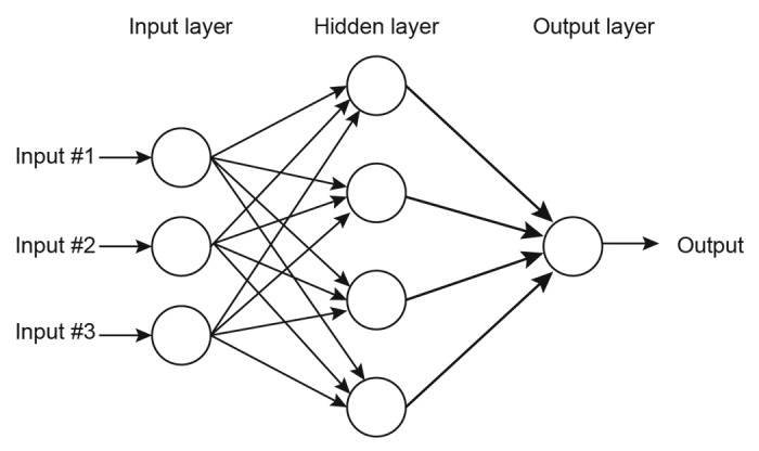
Figure 3. Structure of a typical 3 layer feed forward multilayer perceptron artificial neural network.

The inputs to a neuron are roughly analogous to the dendrites of a biological neuron, and the output of the neuron is comparable to an axon.³⁶ The artificial neuron and its biological counterpart are shown graphically in Figure 4A and B respectively.

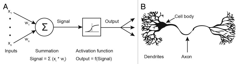
Figure 4. Neurons. (A) An artificial neuron from the hidden or output layer of an MLP, and (B) a simplified depiction of a naturally occurring biological neuron.³⁵

The neurons of the input layer carry out no processing on the values they receive, and merely pass the input values to the next layer along the synapses. Each neuron in the hidden and output layers take the sum of the values on each of its input synapses multiplied by the weight value associated with each synapse to generate the “activation” of the neuron. An “activation function” is applied to the sum to produce the output of each neuron.³⁷

Many of the MLP training algorithms require the use of a differentiable activation function for calculating weight adjustments for hidden layer neurons. The sigmoid is usually favored as its derivatives and partial derivatives can be easily and efficiently produced, which are relevant to typical gradient descent approaches as will be discussed later. Efficiency is important as these values may need to be calculated thousands or perhaps millions of times in teaching an ANN for non-trivial problems. An example of a sigmoidal plot is given in Figure 5. The sigmoid maps the activation of a neuron to a continuous output value in the range 0 to 1 (although the value never reaches 0 or 1).³⁸

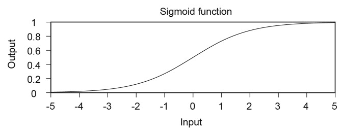
Figure 5. A sigmoid function. If this sigmoid was used as an activation function, the activation of the neuron would be a value on the x-axis and the corresponding output of the neuron is mapped to the y-axis.

Additional inputs with a constant value of 1 are connected to each hidden and output layer neuron. These inputs are referred to as biases. Adjusting the synaptic weight of the bias is equivalent to moving the center of the activation function.³⁹

Alternative architectures to the feedforward MLP are available. For example, Chen and Lukasz provide an introduction to the application of two prominent alternative architectures to protein bioinformatics problems; recurrent and radial basis function (RBF) networks.^14,40 In the generalized form of the MLP, synaptic connections are allowed between neurons in non-successive layers.⁴¹

Training

There are many approaches to training neural networks, but the most typical is a supervised approach in which exemplars of the input to output mappings are used to train the network by adjusting the synaptic weights.¹⁸ Training is an iterative process. Weight updates can be made based on the error of each individual exemplar (online learning) or based on the error of a number of exemplars (batch learning). In each iteration;

• A set of exemplars is applied to the network and the output recorded

• The error of the network is quantified (using an error function)

• The weights of the synapses are then slightly adjusted so that the error of the network would be lower if the same set of training instances were re-applied

In machine learning, a single pass through the entire training set is referred to as an epoch. Through repeated adjustment of the synaptic weights, the network eventually settles on a configuration where no slight adjustments to the weights will result in a net decrease in the error value across the set of exemplars.⁴²

Gradient descent learning is one approach to identifying how the synaptic weights should be adjusted.⁴³ Gradient descent learning uses the idea of an “error surface” which maps the error of a network as a function of the weights.⁴⁰ On the error surface, the slope of the partial derivative of the error of the network with relation to the value of a single weight can be used to identify if a weight should be increased or decreased to lower its error contribution.⁴⁴ An example error surface is shown in Figure 6 for a single weight plotted against network error.

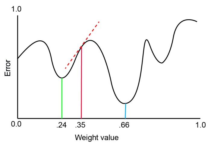
Figure 6. An example of a simulated error surface. The value of a weight (on the x-axis) plotted against the error of the network (the y-axis). The solid red line represents the initial value of a synaptic weight. The dashed red line represents the slope of the error. The green line is a locally minima, a locally optimal weight value. The blue line is the globally optimal value for the weight at which the error contribution is minimized.

The initial values of a synaptic weight give a point on the error function (e.g., 0.35 in Fig. 6). The slope of the derivate of the initial weight value is shown as the dashed red line. A positive slope (as in Fig. 6) indicates that the error contribution can be reduced by reducing the weight value slightly (moving the weight value left along the x-axis). Conversely, a negative slope indicates that the weight value should be increased. By iteratively adjusting the value of the each weight slightly in the direction of its negative of the gradient of the error surface, the error produced by the network can be reduced to a point.⁴³ For Figure 6, the value of the weight would be reduced gradually until it reaches a minimum of the error surface at a value of 0.24. At this point, any small change to the value of the weight should increase the error produced by the network on the training set.

A learning rate, α, is specified to set how much the weights are adjusted each generation. The learning rate should be low to allow the learning algorithm to edge toward the optimal solution.⁴⁵ A learning rate that is too high will cause the adjustments to overshoot minima, making optimization difficult for the algorithm. Of course, a learning rate that is too low will cause slow convergence of the weights, and perhaps lead to the algorithm being unable to escape shallow local minima. A momentum rate can also be specified to increase learning speed by increasing weight adjustment size if consecutive adjustments are in the same direction.⁴⁶

The Feedforward Backpropagation Learning Algorithm

The contribution of a neuron on the output layer to the error of the network can be easily calculated as the difference between the expected and actual output. The contribution of the hidden layer neurons to the error is more difficult as they can may partially contribute to the error of many neurons in successive layers. The back propagation of errors (backpropagation, “Back-Prop” or BP) is a common mathematically provable gradient descent learning algorithm which uses differentiable activation functions to calculate the error of neurons and produce synaptic weights adjustments which reduce this error.¹⁸

If a sigmoid activation function is employed for the neurons of the hidden and output layers, the error signal and weight adjustment calculations can be reduced mathematically to the efficient forms given in Equations 1–4.³⁸ For a more in-depth discussion of how these equations are derived, and a walk through of the first two iterations of weight updating for a simple example network, see the text “Neural Networks” by Phil Picton.⁴⁷ For an output layer neuron k, the error signal, e_k can be calculated using Equation 1 as a function of the difference between the expected output, t_k, and the observed output, o_k. New values for the synaptic weights feeding into k can then be calculated using Equation 2.³⁶

e_k = (t_k − o_k)o_k(1 − o_k) 1

w_ik = w_ik + αe_kx_i 2

Where w_ik and x_i are the weight and input signal respectively of a single synaptic input to the output neuron k, and α is the value of the learning rate constant.

The error signal of a hidden layer neuron must be considered respective of the error of all output layer and other hidden layer neurons to which it feeds its own output.^18,48 To calculate the error signal, e_i, for a hidden layer neuron i, we first define the variable errSum as the summation of the error of each neuron to which i feeds its output, scaled by the synaptic weight connecting them. The error of i can be calculated using Equation 3, and the new synaptic weights feeding into i can be generated using Equation 4.³⁶

e_i = y_i (1- y_i) * errSum Eq. 3

w_ji = w_ji + αe_ix_i Eq. 4

Where w_ji and x_i are the weight and input signal respectively of a single synapse input to the hidden layer neuron i, y_i is the output of neuron i, and α is the value of the learning rate constant. For a more in depth discussion of the mathematical principles and theory of the back propagation algorithm, the reader is directed to the paper “Neural Networks,” by Yang.¹⁶

An interesting variation of backpropagation is the quick prop algorithm.⁴⁹ In quick prop, two iterations of BP are run and the points on the error surface are recorded. Under the assumption that error surfaces are elliptical in shape, quick prop uses the identified two points to estimate where the nadir of the error surface would be located. The synaptic weights can then be adjusted to jump to the expected optimized value. For many problems, the use of quick prop can reduce the processing power and the number of generations required relative to standard BP.

Stopping Criteria

A number of approaches can be used to decide on the number of iterations for which to run a training algorithm. A simple approach is to continue for only a predetermined number of generations, normally set using domain knowledge or experience, above which it can be reasonable assumed no improvement will be observed, or as the amount of available time or resources allows.⁵⁰ A more dynamic approach is to continue iteratively until the error on the training set drops below a threshold specified a priori, or alternatively, until the error of the network over the entire training set drops by less than a specified value (for example 0.01%) over several generations.⁵¹

These simple approaches are however susceptible to “overtraining,” where the performance observed on the training data may not be representative of the performance of the network on novel data.⁵² As training proceeds, the training algorithm, in an attempt to reduce the error, may start to learn decision boundaries which over-fit the training data. This results in reduced error on the training data set at the expense of the ability to generalize to novel exemplars from outside the training data.⁵³ This implies that the training data are not an accurate gauge of the ANNs error on novel data (resubstitution error).

To address this problem, it is common to divide the available exemplars into two independent sets; the training and testing set.⁵⁴ During training (on the training set), the testing set is continually evaluated by the network, but it is not used to affect the weight adjustment of the synapses. The testing set gauges the generalization ability of the network. If the error on the testing set increases over several epochs, while the error on the training set continues to decrease, it is considered an indication that overtraining is occurring. Training can then be stopped and the network weights reverted to the values at which the testing error was minimized.

The performance of the ANN on the testing data cannot be used as an accurate gauge of accuracy either, as the training may have stopped at a point at which the ANN overfits the testing data. For this reason, a third independent set of exemplars, referred to as the validation set, is required to accurately measure the ANN error.⁵⁴

Training an ANN for non-trivial problems can be computationally expensive, perhaps requiring thousands of updates to each synaptic weight. This can correspond to long training times. Florido et al. have described a method of sampling representative exemplars suitable for training an ANN from data sets. It is claimed that such a reduced (but representative) set of training data has the potential to improve training time and reduce overfitting.⁵⁵

Advantages and Disadvantages of ANNs for Bioinformatics

The case for the use of ANNs can be made by their proven successful application to a number of challenging problems in bioinformatics and other domains. Here, the strengths of ANNs, weaknesses, and reasons why they are appealing for bioinformatics problems are discussed.

Advantage: Generalization

Generalization in machine learning refers to the ability of the solution to extrapolate good outputs for unseen data or new combinations of inputs based on what it has been trained on. The generalization ability of ANNs is well documented, and is one of the strongest and most desirable qualities for bioinformatics, although it is a quality shared with many other machine learning and model based approaches.

Strong generalization is a highly desirable in many situations in the bioinformatics domain. For example, often experiments can produce gigabytes of data, but diseases and conditions can present differently in different environments. Expression levels of a biomarker gene, for example, may vary depending on the age, gender, health, race, etc. of a patient. Generating data to cover all permutations of even these four contributing factors may be time consuming, expensive or just not possible for rare conditions. Using only a sampling of these permutations, an ANN can often learn how these attributes affect the observed biomarkers, and learn to correctly classify (or at least make a very well informed guess) as to the classification of patients whose combination of attributes were not covered by the training data.

Advantage: No Need for Complete Domain Knowledge

Another appealing property of ANNs for bioinformatics is that domain knowledge does not need to be complete. There are also situations where exact solutions exist, but ANNs can be used to estimate the desired output where generating the exact solution is prohibitive in terms of cost or time. Protein folding is an example of a problem which is not fully understood, but to which ANNs have been applied with a good level of success. The 3D structure of a protein can be generated using X-ray crystallography, but this is a very time consuming approach, so not suitable for the vast amount of sequences which can be generated in a single bioinformatics experiment.

An ANN can be trained to hypothesize protein structure based on primary sequence alone (which can be identified much more quickly and cheaply), given the structure of a number of exemplars which may have been identified using X-ray crystallography. ANNs achieve this success without the need to understand the underlying mechanisms, but can examine how known contributing factors have affected the structure of proteins with identified form to conjecture how a novel chain will be affected. The application of ANNs to protein folding is discussed in more detail in the case studies section.

Advantages: Robust Solutions to Complex Problems

The third main advantage of ANNs for bioinformatics that we will discuss is the general robustness of the solutions that can be produced and the complexity of the problems to which it can successfully be applied. We demonstrate these points collectively by considering an example of how neural networks have been applied to microarray data.

Generic microarrays covering a large number of genes can have a low statistical power due to the small sample sizes (number of arrays available) and high levels of noise (mismatch binding and contamination) typical in microarray experiments. Genes identified as differentially expressed in one experiment may not appear differentially expressed in another experiment. In fact, it has been demonstrated that thousands of microarray samples may be required to define reproducible biomarkers with confidence in some situations.⁵⁶

ANNs are a technology which has provided good performance on microarray data in spite of the limitations of the arrays, by using readily available information from multiple heterogeneous sources to place meaning on the observed experimental results. Using the assumption that deregulated proteins are as a result of, or cause, deregulation of the proteins with which they interact, Chuang et al. demonstrated that the information in protein-protein interaction (PPI) networks can be combined with microarray data to define more robust biomarkers.⁵⁷ This approach evaluates the aggregate behavior of sub-networks of interacting genes (connected within the PPI network), allowing the relevance of genes with subtle differential expression can be combined to produce more reproducible and robust biomarkers.

The CRANE algorithm is an example of such an approach, which employs an ANN to perform classifications based on identified disregulated PPI subnetworks.⁵⁸ The expression levels of the genes in the subnetworks form the inputs to the ANN. The use of these subnetworks of related genes is shown to outperform groups of genes selected based on experimentally observed differential expression alone in classification problems. This example demonstrates how ANNs applied in the bioinformatics domain can:

• Consider the impact of many attributes (capable of relatively high dimensionality) from multiple heterogeneous sources

• Work with multiple patterns (can use multiple PPI networks in generating its output, with potentially both positive and negative biomarkers)

• Consider the impact of even low impact attributes which may or may not even be present.

• Can produce robust fault tolerant solutions which, to a degree, can handle contamination, low statistical power, effects of machine calibration, background noise, and repeatability of experiments observed in the data sets, all of which can be inherent in data generated from generic microarrays

• As discussed earlier, gene expression levels can also be impacted the gender, age, race, etc. of the patient, but this can be addressed by the strong generalization ability of ANNs.

For a detailed discussion of the application of ANNs to microarrays we suggest the paper “An introduction to artificial neural networks in bioinformatics-application to complex microarray and mass spectrometry datasets in cancer studies” by Lancashire, Lemetre and Ball.¹⁵

Disadvantage: Local Minima

Learning algorithms such as back propagation are applied with the caveat that solutions may only be locally as opposed to globally optimal.⁵⁹ In Figure 6 it can be seen that gradient descent starting at the initial point on the error surface (weight value 0.35) will adjust the weight value to a point where the error is reduced (weight value 0.24), but not necessarily to the value of the weight where the error is minimized. The point of lowest error on the error surface is referred to as the global minimum of the error surface and is given by a weight value of 0.66 for the example of Figure 6. The inability of gradient descent algorithms to consistently identify global minima is referred to as the local minima problem.^60,61

This problem can be lessened by repeating training several times with different initial weight values (and therefore different starting points on the error surface),⁶² or through processes such as simulated annealing⁵⁹ or neuroevolution.⁶³

Disadvantage: Selecting the Architecture

Whereas the number of input and output neurons is prescribed by the cardinality of the required mapping, the number of hidden layers and the number of neurons in each hidden layer is dictated by the complexity of the problem, and is typically empirically defined.^64-66 Although this is still considered an unsolved task, Xu and Chen overview several opinions and approaches to the selection of appropriate architectures.⁶⁷ If too few neurons are present the potential complexity of the decision boundaries produced by the network will be limited (“under-fitting”),⁶⁸ while too many neurons will encourage the network to overtrain by allowing overly intricate decision boundaries.⁶⁹

One approach to this problem is neuroevolution; the use of evolutionary algorithms to discover good neural network architectures in an automated fashion.⁷⁰ These evolutionary algorithms are not guaranteed to find the optimal solution, but should find a good solution in a reasonable amount of time.⁷¹ Topology and weight evolving artificial neural network (TWEANN) algorithms such as the NeuroEvolution of Augmenting Topologies (NEAT)⁶³ and Cartesian Genetic Programming Evolved Artificial Neural Network (CGPANN)⁷² variations have recently shown good performance on bioinformatics data sets.^73-75

Disadvantage: Not Always the Best Approach

In comparative analyses, ANNs generally perform well, but do not necessarily offer the best performance. For example, in the paper “Why neural networks should not be used for HIV-1 protease cleavage site prediction” it is demonstrated that although ANNs are capable of classifying linearly separable data, superior performance is achieved by linear classifiers when applied to linear problems.⁷⁶

Additionally, alternative machine learning approaches exist which have proven more effective than ANNs on a number of problems. Isroy et al. have performed a survey of papers dealing with machine learning based classification from three bioinformatics journals over 2010 and 2011.⁷⁷ It was observed that, of the papers surveyed, 13% employed artificial neural networks, while 57% employed Support Vector Machines (SVM). The findings of Isroy et al. are presented in Table 1.

Table 1. Use rates of different machine learning algorithms in a sampling of bioinformatics papers, as presented by Isroy et al.⁷⁵.

Algorithm	Percentage (2010)	Percentage (2011)	Percentage (2010–2011)
Decision Tree (DT)	26	24	26
Support Vector Machine (SVM)	51	69	57
Rule Based Learning	4	3	4
Artificial Neural Network (ANN)	10	17	13
Naive Bayes (NB)	16	14	15
k-Nearest Neighbor (KNN)	15	17	15

Chan et al. compared the relative performance of the MLP and two SVM variations in terms of receiver operating characteristic (ROC) and sensitivity at set specificity levels on a glaucoma diagnosis data set.⁷⁸ The approaches are evaluated using the full set of attributes and a reduced set identified using principal component analysis (PCA). The results (presented in Table 2) show the SVM out-performing the MLP on this problem.

Table 2. Performance of the MLP and SVM on Glaucoma diagnosis, as presented by Chan et al.⁷⁶.

			Sensitivity at specificity of
		ROC area	0.9	0.75
Full	MLP	0.883	0.66	0.859
	Gaussian SVM	0.914	0.776	0.878
	Linear SVM	0.893	0.66	0.853
PCA	MLP	0.898	0.713	0.846
	Gaussian SVM	0.904	0.744	0.833
	Linear SVM	0.888	0.667	0.853

ANNs are however still a very powerful tool, and numerous papers can be identified where the ANN matches or outperforms the SVM approach. Chowdhury et al., for example, in describing the CRANE algorithm discussed previously, argue that how ANNs deal with sub-patterns makes them better suited to that problem than SVMs.⁵⁸

Cho and Ryu compared the performance of MLPs and two variations of the SVM in combination with a number of feature selection algorithms on gene expression profiles.⁷⁹ These results are presented in Table 3. It is noted that, on this data set, the MLP consistently performed as well as or better than the SVM approaches. The MLP also performed favorably compared with the self-organizing map (SOM), decision tree (DT) and k-nearest neighbor (KNN) algorithms (data not shown). Further work by Cho and Won produced similar results for Leukemia, colon and lymphoma data sets.⁸⁰

Table 3. Comparing the performance of the MLP with the SVM on gene expression data in combination with different feature selection algorithms.

	Pearson	Spearman	Euclidean distance	Cosine coefficient	Information gain	Mutual information	S/N ratio
MLP	97.1	70.6	97.1	79.4	72.9	62.1	94.1
SVMRBF	97.1	70.6	91.2	70.6	58.8	58.8	94.1
SVMlinear	79.4	70.6	88.2	58.8	58.8	58.8	94.1

Chang et al. directly compared the performance of the MLP and SVM on the classification of breast tumor images. Their results noted that the MLP and SVM have comparable accuracy (see Table 4), but the SVM could be trained much quicker.⁸¹

Table 4. The performance of the MLP and SVM on the task of identifying breast cancer from image data.

	SVM	MLP
Accuracy (%)	85.60	84.80
Sensitivity (%)	95.45	84.55
Specificity (%)	77.86	77.14

Implementations

There are a number of freely available open-source ANN implementations (in many programming languages) available through sites such as Google Code, Sourceforge and Github. The WEKA project (Waikato Environment for Knowledge Analysis) is an open-source implementation of a library of different machine learning algorithms. Implementations in the R programming language are hosted on the site http://cran.r-project.org/.

Case Studies

In the following section, we present a number of varied example applications of ANNs to bioinformatics problems. We do not advocate that these approaches necessarily represent the best approaches or practices, but rather they serve as examples of how the principles of ANNs can be applied to different real world bioinformatics problems.

Peptide Secondary Structure Prediction

A protein comprises of a chain or multiple chains of amino acid residues.⁸² The chemical properties of the amino acids in the peptide cause the chain to twist and fold into a number of regular structures to form a stable three-dimensional conformation.^83,84 It is this three-dimensional conformation of the chains which designate the function of the protein.^85,86 The structure of a protein is defined at several levels;⁸⁷

• Primary structure: the order of the amino acid residues which constitute the protein

• Secondary structure: the locations and identities of a number of regular local secondary structures along the primary structure of the protein (such as the α helix and the β strand)

• Tertiary structure: the overall three-dimensional conformation taken by a single peptide chain

• Quaternary structure: complexes formed from several peptide chains link together which act as a single protein

Example: Sequence Similarity Based Secondary Structure Prediction

Rao et al.⁸⁸ gave an approach to identifying the secondary structure of a peptide given its primary structure using an ANN. The main idea behind the approach is that segments of a peptide chain with similar primary sequence are assumed to have similar secondary structure expressions. Under this assumption, the secondary structures for novel amino acid sequences can be generalized from similar amino acid sequences with known secondary structure classifications.

To identify the secondary structure of an amino acid, a window of between 15 and 29 neighboring amino acids are used as the input to a neural network. The identity of each amino acid in the window is encoded using 20 inputs to the network. For a window of size W, the ANN is a single layered MLP with W*20 input neurons, W*2 + 1 hidden layer neurons, and 8 output neurons representing different structural designations. The secondary structure classification for an amino acid residue is therefore given as the classification corresponding to the highest output on the network. For example, if the first output of the network has the highest output, the amino acid residue under investigation is designated as an α-helix. If the last output of the network has the highest value, the amino acid residue is designated as a coil. The network is trained using the scaled conjugate gradient descent algorithm.⁸⁹

The network was trained using data taken from the DSSP database, which contains peptide sequences and their corresponding secondary structure classifications.⁹⁰ In evaluations on a single sequence, the network achieved a Q₈ score of 72.3%, meaning it correctly classified 72.3% of the amino acid residues as belonging to the correct one of the 8 possible secondary structure classes.

Example: PSIPRED

PSIPRED is an application which predicts a proteins secondary structure from its primary structure using a pair of artificial neural networks trained using BP. For a given sequence, PSIPRED uses a “sequence profile” to examine how highly preserved elements of the sequence are relative to homologs and distant homologs identified from a database. Matching against the sequence profile is more relevant than the sequence itself, as functional regions of peptides tend to display a high level of preservation, but also as regions with high sequence similarity identified in the database may be purely coincidental. PSIPRED uses position specific scoring matrixes (PSSMs) generated as a by-product of another program, PSI-BLAST, to present this information to the first neural network.

BLAST is a tool for finding homologous multiple sequence alignments from a database for a given sequence.⁹¹ For a sequence of length n, n − w + 1 words of length w can be generated. The database is then searched against each word using a finite state machine. Words are evaluated using a substitution matrix, and words scoring above a threshold T are extended in both directions. Position specific iterated BLAST (PSI-BLAST) makes a number of improvements over standard BLAST.⁹² One of the improvements is that once the original sequence alignment is completed, the identified similar sequences are used to form a PSSM of size 20× n. The process can then be repeated iteratively, where the PSSM generated in each iteration is used in place of the original substitution matrix. This iterative process allows the discovery of distant homologs from a database.

PSIPRED generates a classification for an amino acid as one of 3 secondary structure states (Q₃); a helix, strand, or loop.⁹³ The Q₃ training and testing data are generated from the DSSP database Q₈ classifications (as used in the sequence similarity based approach) using the approach specified by Rost and Sander.⁹⁴ To generate the Q₃ value for an amino acid in a given sequence, a sub-sequence is first generated comprising the amino acid and a window of 7 amino acids to either side.⁹⁵ This subsequence is then fed into PSI-BLAST. The values of the PSSM generated by PSI-BLAST after 3 iterations are used to generate 300 inputs (15 × 20) to the first ANN. An additional input is associated with each amino acid in the window representing if that amino acid spans the N or C terminus. The first ANN has a single hidden layer with 75 neurons, and 3 output layer neurons each representing an individual Q₃ classification. The output with the highest evidential response is taken as the classification of the amino acid at the center of the window. This process is shown in Figure 7.

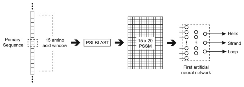
Figure 7. Generating a Q3 classification for a specific amino acid (in the dashed box) using the first ANN of PSIPRED.

Once the first network has been applied to classify the entire sequence, a second neural network with 60 hidden layer neurons and 3 outputs is used to further refine the results.⁹⁵ To classify an amino acid in the sequence, the outputs of the first network for the window of 15 amino acids is used as input to the second network. Again, an additional input is added as previously for each amino acid in the window representing if the amino acid spans the N or C terminus. The output of the second network is still the Q₃ classification of the central amino acid, but this network tends to be more accurate in deciding a conformation for an amino acid given likely conformations of its direct neighbors. These steps are shown graphically in Figure 8.

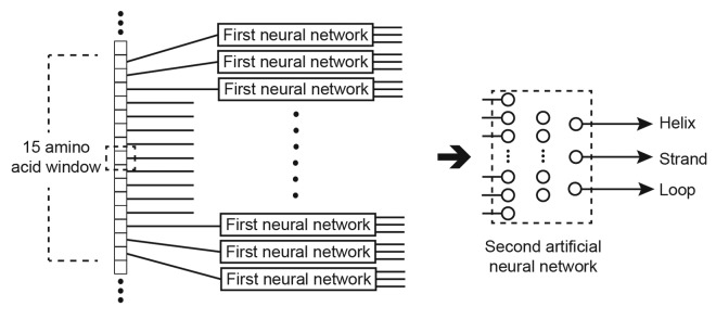
Figure 8. Improving the accuracy of the Q3 score using a second ANN.

PSIPRED was independently evaluated in the CASP3 (Third Critical Assessment of Structure Prediction) competition, where it was identified as the top performing approach across a number of blind evaluations.⁹⁶ PSIPRED version 2.0 also performed well in CASP4.⁹⁷ PSIPRED 3.2 claims to achieve an average Q₃ score of 81.6% (http://bioinf.cs.ucl.ac.uk/index.php?id=779).

Gene Identification

Neural networks have previously been applied for the categorization of coding (exons) and non-coding (introns and intragenic spacer data) regions of a DNA. For an overview of eukaryote gene prediction strategies see Sleator.⁹⁸

Example: Gene Identification Using Coding Measures

An interesting example of this is the approach taken by Fogel, Chellapilla, and Fogel, who construct an ANN using neuroevolution to classify nucleotides as coding or non-coding.^99,100 This work builds on network inputs identified by Uberbacher and Mural for the GRAIL application.¹⁹

As for many gene identification techniques, the window is pre-processed to extract features of the sequence, known as “coding measures.”¹⁰¹ Coding measures are statistical observations on the differences in distribution and repeated patterns of the nucleotides in coding and non-coding regions of DNA. These statistics present an opportune training set for neural network architectures; an established mapping that can be used for training a network to differentiate coding gene sequences on novel input. As such, the neural network is employed to define a nonlinear weighting for each of the coding measures, and allowing the consideration of how these coding measures can affect probability when observed under various combinations.

The “frame bias matrix” is an example of a coding measure that works at the nucleotide level. The frame bias matrix works on the observation that the four nucleotides (ACGT) have different probabilities of being observed in the three codon positions for both coding and non-coding regions.¹⁰² Therefore, the presence of specific nucleotides in codon locations can be considered as positive or negative indicators for the codon being in a coding region.

The “coding sextuple word preferences” coding measure works on the principle that certain sextuple nucleotide combinations can be identified which occur more frequently in coding regions of DNA.¹⁰³ An instance of this would be the sextuple ACCGTA in the coding sequence CACACGACCGTACTCACAT. Through examining known coding and non-coding regions, n-tuples words can be identified which have higher probabilities of being observed in either coding or non-coding regions of DNA.

Many coding measures are available, but this approach specifies the use of nine to form the input to the ANN; 2 at the nucleotide level and 7 at the word (n-tuple) level.

• Frame bias matrix

• Fickett Feature

• Coding Sextuple word preferences

• Coding sextuple in-frame word preferences

  • Word preferences in frame 1

  • Word preferences in frame 2

  • Word preferences in frame 3

• Maximum word preferences in frames

• Sextuple word commonality

• Repetitive Sextuple word

To evaluate a nucleotide, a window of 99 nucleotides is isolated. The nucleotides in the window are pre-processed to generate the coding measures, which are then fed into the ANN. The network is a fully connected MLP with 14 hidden layer neurons and a single output representing the derived classification. The flow of data for this approach is demonstrated in Figure 9. Post-processing is performed on the output of the network to improve performance using domain knowledge.

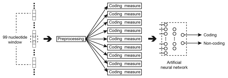
Figure 9. Classifying a nucleotide (in the dashed box) as coding or non-coding using an ANN.

The synaptic weights of the ANN, in this situation, were trained using an evolutionary algorithm, which is itself a nature inspired machine learning algorithm. In this evolutionary algorithm, large populations of potential solutions (in this case, sets of synaptic weights) are created and evaluated. In each generation, half of the potential solutions with lower performance are purged, and the survivors are used as the basis for a new population of the original size. The candidate solutions for the new population are created by modifying a single weight from a solution of the previous generation which showed good performance. In this way, over many generations useful elements of successful solutions be propagated and increasingly more successful networks should be created. The large space of potential solutions evaluated tend to produce an optimal (if not the optimal) network solution. 250 000 examples of coding and non-coding nucleotides were used to train the network, with the mean squared error and correct classification percentages used to select the best performing each generation.

The performance of this ANN based approach to gene identification was evaluated on two sets of human DNA sequences taken from GenBank. It has been reported that the network classified the majority of coding nucleotides correctly with sensitivity (the ratio of true positives to the number of true positives and false negatives) of 74% and 64%, outperforming a number of other systems. In particular, the authors of this study note that 1.4 times more true positives were observed for this approach compared with the GRAIL server on the same data. However, it was also reported that the network had a high false positive rate (some non-coding regions incorrectly as coding regions), resulting in a specificity (the ratio of true negatives to the number of true negatives and false positives) of only 38% and 42%. The authors attribute this over sensitivity to coding sub-sequences on the composition of the data used to train the network, as it was split equally between coding and non-coding exemplars, which does not reflect real world sequences where it is estimated that only 2% is coding.¹⁰⁴

It is noted by the authors that a system that reports false positives is preferential to a system that reports false negatives as it will be less likely to miss coding regions. On the other hand, a system that has a higher ratio of false negatives will report coding regions as being non-coding and so they will be potentially excluded by researchers from further study.

Example: Neural Network for Promoter Prediction (NNPP)

A common problem for neural networks is detecting transient patterns which can occur at any point over a subsection of an input signal. An example of this is promoter binding sites, which can occur anywhere in a window of nucleotides relative to the transcription start site (TSS). Typically, this problem can be addressed by (1) training a network with exemplars of the pattern at all possible locations, or (2) training a network on specific exemplars of the pattern and applying the network brute force to every point in the input space where the pattern may occur. The Time delay neural network (TDNN) is a structured approach to this problem, which combines elements of both these methods.¹⁰⁵

TDNN was originally applied for detecting the presence of specific phonemes from speech samples. The TDNN operates by learning feature detectors (the hidden layer neurons) for patterns which are replicated to cover the input signal in a continuous overlapping manner.¹⁰⁶ Each feature detector examines only a subsection of the input signal, referred to as the detector’s receptive field. The activation of all the feature detectors is then combined to determine if the desired pattern is identified anywhere in the signal.

TDNN weights are learned using a modified BP algorithm. An input signal is applied to the network in the standard feed-forward manner and BP used to calculate the error and identify the weight adjustment for each synapse. As a set of replicated feature detectors are all looking for the same pattern (but at different points in the signal), a synaptic weight is actually updated as the average weight adjustment (Δ) generated by BP for the corresponding synapse across all copies of that feature detector. This approach means that the actual offset of the pattern in the exemplar signals does not affect training or recognition.

The Neural Network for Promoter Prediction (NNPP) approach employs two of these TDNNs.¹⁰⁷ Given a nucleotide sequence, each TDNN will each examine a different overlapping window of nucleotides for patterns representing a TATA box and initiator box respectively. Both TDNNs are trained separately and subsequently combined to form a super network which can consider the presence or absence of both binding sites and their relative positions to decide if a point in the sequence is a TSS.

The input to the TDNN for identifying an initiator box is a window of 25 base pairs, ranging from 14 base pairs upstream to 11 base pairs downstream of the point in the sequence under investigation. Instead of a time delay as for the standard TDNN, each nucleotide in the window is considered as a time slice in a signal. The initiator box detector TDNN employs a receptive field size of 15 base pairs. Therefore, 11 feature detectors are required to cover all possible 15 nucleotide frames in the window, as demonstrated in Figure 10. Each base pair is encoded in four binary bits, so each feature detector will receive 60 (4*15) synaptic connections, connecting it to a subset of the window. The TDNN for detecting TATA boxes works in exactly the same manner, but examines a window of between 40 base pairs upstream to 10 base pairs upstream of the point in the sequence under investigation.

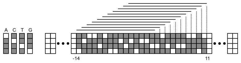
Figure 10. The windowed subsection of the input sequence and the receptive frames for the initiator box. Each receptive field frame is connected to a separate feature detector.

The NNPP was tested on the Adh region of the Drosophila genome. The data set comprised 2.9 million nucleotides with 92 annotated promoters. The NNPP super-network accepts a window of 51 bases comprising the two overlapping windows used by the pair of hidden layers. The window is moved along the entire sequence and a score generated for each nucleotide as a TSS. The scores are post-processed using a simple smoothing function as part of the NNPP process. The NNPP approach correctly identified 69 of the 92 known promoters (Sensitivity of 75%), and achieved 99.82% specificity. If a more exacting threshold was applied to only accept promoter classifications where the NNPP has a confidence in the prediction of greater than or equal to 97%, the specificity increased to 99.96% (1 false positive per 2416 nucleotides), but the NNPP could still successfully detect 38% of the known promoters.

Although the results produced cannot account for all promoter regions, the low levels of false positives observed have helped NNPP find a great number of applications in identifying and verifying putative TSSs, often to compliment other TSS identification approaches.^108-112

Gene-Gene Interaction

Genome wide association studies (GWAS) are used to identify genetic risk factors for common diseases. Genetic association studies directly compare the sequences of genotypes between target (displaying a specific trait or condition) and control populations. Any single nucleotide polymorphisms (SNP) common in the target group and rare in the other is taken as a likely contributing factor. Although examining individual SNPs in isolation has identified many genetic risk factors across a range of conditions such as type II diabetes and HDL-cholesterol, this approach has not been able to explain much of the causation thought to be attributable to genetic variation. Examining the target population in terms of epistasis (two or more interacting genes) is significantly more difficult because of the “curse of dimensionality”; as the pre-requisite for the situation (disease) becomes more complex, the amount of representative data becomes reduced and more difficult to identify. Additionally, epistatic interactions are typically observed with low effect sizes.

Example: ATHENA

ATHENA (Analysis Tool for Heritable and Environmental Network Associations) employs a neural network as a means of data mining such gene-gene interactions from genome wide association studies.¹¹³ Data mining is the process of discovering unknown patterns from large data sets, in this case the identification of the epistatic SNPs among a large number of unrelated SNPs.^114,115 This approach uses a form of neuroevolution, grammatical evolution neural networks (GENN), to efficiently search the space of possible network inputs (feature selection) without the need for brute-force trial of all possible two locus SNP combinations.

Similar to the approach of Corne et al. described previously, the GENN used in ATHENA is a form of evolutionary algorithm which evolves a population of differing neural network solutions, but GENN also attempts to evolve the architecture of the network.¹¹⁶ Combinations of inputs and hidden layer neurons which show relevance to predicting potential disease cases are replicated and disseminated across increasing solutions over the following generations. Crossover and mutation are used to evolve new generations of the population. Allele variations, which form the inputs to the network are encoded as (−1, 0, +1) representing the three forms of a gene with an SNP (AA, Aa, aa).

The process was evaluated in silico using a simulation study for accurate evaluations of the process such that the true effect of each SNP is known and understood. The exemplars were generated with epistasis occurring under two models; the additive and dominant models. Under the additive model for example, the penetrance of a disease is increased as a function of the number of recessive alleles; i.e., for AABB penetrance will be at a minimum, but at a maximum for aabb. Two thousand exemplars are generated using the genomeSIMLA application. Each exemplar consisted of 2 epistatic SNPs and 498 irrelevant (to the particular disease penetrance) SNPs. Narrow-sense heritability was set at only 5% in the generated data, meaning very few of the case exemplars display the epistatic trait. The low epistatic effect size is typical of real world data. A 1% main effect is simulated for each of the epistatic loci.

In some of the trials, a hybrid learning approach was used in which the BP algorithm trained the initial network population, and again after a number of generations. BP was run for a maximum of 100 epochs on each network. The authors also investigate the use of existing domain knowledge as a means of filtering the search space. This domain knowledge for the experiment is again simulated, mimicking the scores produced for SNP pairs generated by the Biofilter application. Biofilter examines available databases for published information which supports the selection of pairs of SNPs.¹¹⁷ The higher the implication score generated by Biofilter, the more support that can be found for that SNP pair. This implication level is simulated in the data by generating 4000 random edges.

Trials were performed under differing implication levels, differing proportions of the population intelligently initialized using the domain knowledge, and in the presence of absence of backpropagation. To test each combination of these parameters 100 data sets were generated. Sensitivity was defined as the proportion of those 100 data set for which the best performing network identified (accepted as inputs) only the two SNPs generating the epistasis in the data set. The results attained by Turner et al.:

• Demonstrate the ability of neural networks to identity and model nonlinear interaction in data sets in spite of low effect levels (5%) and in the presence of substantial levels of noise

• Display the potential for efficiency gains when domain knowledge is incorporated into large search spaces, which is extremely important in the case of large scale problems such as genome wide association studies

Conclusions

Neural networks are a potentially powerful tool for bioinformatics, with reported successful applications across many areas and levels of the domain. The example applications given here show ANNs as being able to identify and model complex patterns and manage large data sets, which can be both sparse and noisy.

The theory of neural networks is still evolving as the problems faced are changing. For example, Hawkins’s Hierarchical Temporal Memory (HTM) is an ANN model suggested as an alternative to storing large amounts of data common in commercial and bioinformatics domains.¹¹⁸ Built on an improving understanding of how the brain works, the HTM is a rough approximation of how layer 3 of the neocortex operates. It is a more biologically plausible ANN, which attends that the brain is a memory system as opposed to a processor (as with MLPs). The approach postulates that data in many domains decreases in relevance as it ages. Instead of storing all the data, the HTM builds a model encoding the patterns in the data, and constantly updates the model as new data becomes available. The HTM is capable of Identifying and modeling spatial (combinations that occur together) and temporal (spatial patterns occur together over time) patterns, and detecting anomalies in large data sets.¹¹⁹

Another area of ANN research which is gaining in popularity as its power is being full understood, is the idea of a “deep neural network”¹²⁰ (DNN); neural networks comprising many hidden layers. These deep network architectures can be powerful, but the typical backpropagation algorithm can struggle or become intractable when it is required to learn many hidden layers, as the error signal being back propagated is constantly reducing.^121,122 Hinton et al. describe a variation of the restricted Boltzmann machine (RBM) neural network approach capable of learning many layers,¹²³ where each layer is a further abstraction of features in the training data.^124,125 These feature abstractions of the network are trained to encode an input signal (the training exemplars) through a number of layers, and decode it back through the network to be able to replicate a good approximation of the original signal. In bioinformatics, a common problem is the lack of classified data. Generative models, such as Hinton’s RBM can be used to mitigate this issue, as it can handle the difficult problem of learning these abstractions without the need for labeled data.¹²⁶ A smaller amount of labeled exemplars can be used to train the network to act as a classifier.

ANNs may not always be the best approach to solving a problem. Although ANNs work in the absence of key domain knowledge, significant domain knowledge can be required in selecting the inputs and knowing how best to pre-process the input values. However, identifying what is relevant is often an easier task than defining how these values should be interpreted. If a problem is well understood, and can be addressed using a set of known and understood rules, this can be favorable or less error prone than the decisions or interpretations of stimuli produced by a neural network. There is also the need for a sufficient amount of accurately classified training data to be available to adequately describe the remit of situations the network must learn, which may not be readily available.

Glossary

Abbreviations:

ANNs

artificial neural networks

MLP

multi-layer perceptron

BP

backpropagation

TWEANNs

topology and weight evolving artificial neural network algorithms

NEAT

NeuroEvolution of augmenting topologies

CGPANN

Cartesian genetic programming evolved artificial neural network

BLAST

Basic Local Alignment Search Tool

PSI-BLAST

Position specific iterated-BLAST

GWAS

Genome wide association studies

ATHENA

Analysis Tool for Heritable and Environmental Network Associations

GENN

grammatical evolution neural networks

HTM

Hierarchical Temporal Memory

RBM

Restricted Boltzmann machine

PPI

protein-protein interaction

ROC

receiver operating characteristic

HTM

hierarchical temporal memory

DNN

deep neural network

PSSM

position-specific scoring matrix

10.4161/bioe.26997

References

- 1.Durda K, Buchanan L, Caron R. Grounding co-occurrence: Identifying features in a lexical co-occurrence model of semantic memory. Behav Res Methods. 2009;41:1210–23. doi: 10.3758/BRM.41.4.1210. [DOI] [PubMed] [Google Scholar]
- 2.Hinton GE, Srivastava N, Krizhevsky A, Sutskever I, Salakhutdinov RR. Improving neural networks by preventing co-adaptation of feature detectors. arXiv preprint arXiv:12070580 2012.
- 3.McEvoy FJ, Amigo JM. Using machine learning to classify image features from canine pelvic radiographs: evaluation of partial least squares discriminant analysis and artificial neural network models. Vet Radiol Ultrasound. 2012;54:122–6. doi: 10.1111/vru.12003. [DOI] [PubMed] [Google Scholar]
- 4.Acharya UR, Vinitha Sree S, Mookiah MR, Yantri R, Molinari F, Zieleźnik W, Małyszek-Tumidajewicz J, Stępień B, Bardales RH, Witkowska A, et al. Diagnosis of Hashimoto’s thyroiditis in ultrasound using tissue characterization and pixel classification. Proc Inst Mech Eng H. 2013;227:788–98. doi: 10.1177/0954411913483637. [DOI] [PubMed] [Google Scholar]
- 5.Mariani S, Grassi A, Mendez MO, Milioli G, Parrino L, Terzano MG, Bianchi AM. EEG segmentation for improving automatic CAP detection. Clin Neurophysiol. 2013;124:1815–23. doi: 10.1016/j.clinph.2013.04.005. [DOI] [PubMed] [Google Scholar]
- 6.Sachdeva J, Kumar V, Gupta I, Khandelwal N, Ahuja CK. Segmentation, feature extraction, and multiclass brain tumor classification. J Digit Imaging. 2013;26:1141–50. doi: 10.1007/s10278-013-9600-0. [DOI] [PMC free article] [PubMed] [Google Scholar]
- 7.Zhao Y, Chen D, Luo Y, Li H, Deng B, Huang SB, Chiu TK, Wu MH, Long R, Hu H, et al. A microfluidic system for cell type classification based on cellular size-independent electrical properties. Lab Chip. 2013;13:2272–7. doi: 10.1039/c3lc41361f. [DOI] [PubMed] [Google Scholar]
- 8.Elfwing S, Uchibe E, Doya K. Scaled free-energy based reinforcement learning for robust and efficient learning in high-dimensional state spaces. Front Neurorobot. 2013;7:3. doi: 10.3389/fnbot.2013.00003. [DOI] [PMC free article] [PubMed] [Google Scholar]
- 9.Firoozpour L, Sadatnezhad K, Dehghani S, Pourbasheer E, Foroumadi A, Shafiee A, Amanlou M. An efficient piecewise linear model for predicting activity of caspase-3 inhibitors. Daru. 2012;20:31. doi: 10.1186/2008-2231-20-31. [DOI] [PMC free article] [PubMed] [Google Scholar]
- 10.Leite D, Costa P, Gomide F. Evolving granular neural networks from fuzzy data streams. Neural Netw. 2013;38:1–16. doi: 10.1016/j.neunet.2012.10.006. [DOI] [PubMed] [Google Scholar]
- 11.Plake C, Schiemann T, Pankalla M, Hakenberg J, Leser U. AliBaba: PubMed as a graph. Bioinformatics. 2006;22:2444–5. doi: 10.1093/bioinformatics/btl408. [DOI] [PubMed] [Google Scholar]
- 12.Roberts RJ. PubMed Central: The GenBank of the published literature. Proc Natl Acad Sci USA. 2001;98:381–2. doi: 10.1073/pnas.98.2.381. [DOI] [PMC free article] [PubMed] [Google Scholar]
- 13.Sleator RD. Digital biology: a new era has begun. Bioengineered. 2012;3:311–2. doi: 10.4161/bioe.22367. [DOI] [PMC free article] [PubMed] [Google Scholar]
- 14.Chen K, Kurgan LA. Neural Networks in Bioinformatics. Handbook of Natural Computing: Springer, 2012:565-83. [Google Scholar]
- 15.Lancashire LJ, Lemetre C, Ball GR. An introduction to artificial neural networks in bioinformatics--application to complex microarray and mass spectrometry datasets in cancer studies. Brief Bioinform. 2009;10:315–29. doi: 10.1093/bib/bbp012. [DOI] [PubMed] [Google Scholar]
- 16.Yang Z. Neural Networks. In: Carugo O, Eisenhaber F, eds. Data Mining Techniques for the Life Sciences: Humana Press, 2010:197-222. [Google Scholar]
- 17.Meireles MR, Almeida PE, Simões MG. A comprehensive review for industrial applicability of artificial neural networks. Industrial Electronics. IEEE Transactions on. 2003;50:585–601. [Google Scholar]
- 18.Rumelhart DE, Hintont GE, Williams RJ. Learning representations by back-propagating errors. Nature. 1986;323:533–6. doi: 10.1038/323533a0. [DOI] [Google Scholar]
- 19.Uberbacher EC, Mural RJ. Locating protein-coding regions in human DNA sequences by a multiple sensor-neural network approach. Proc Natl Acad Sci USA. 1991;88:11261–5. doi: 10.1073/pnas.88.24.11261. [DOI] [PMC free article] [PubMed] [Google Scholar]
- 20.Qian N, Sejnowski TJ. Predicting the secondary structure of globular proteins using neural network models. J Mol Biol. 1988;202:865–84. doi: 10.1016/0022-2836(88)90564-5. [DOI] [PubMed] [Google Scholar]
- 21.Bishop CM. Neural networks for pattern recognition. Oxford university press, 1995. [Google Scholar]
- 22.Kotsiantis S, Zaharakis I, Pintelas P. Supervised machine learning: A review of classification techniques. Frontiers in Artificial Intelligence and Applications. 2007;160:3. [Google Scholar]
- 23.Montana DJ, Davis L. Training feedforward neural networks using genetic algorithms. Proceedings of the eleventh international joint conference on artificial Intelligence: San Mateo, CA, 1989:762-7. [Google Scholar]
- 24.Baba N. A new approach for finding the global minimum of error function of neural networks. Neural Netw. 1989;2:367–73. doi: 10.1016/0893-6080(89)90021-X. [DOI] [Google Scholar]
- 25.Sietsma J, Dow RJ. Creating artificial neural networks that generalize. Neural Netw. 1991;4:67–79. doi: 10.1016/0893-6080(91)90033-2. [DOI] [Google Scholar]
- 26.Razavi S, Tolson BA. A new formulation for feedforward neural networks. IEEE Trans Neural Netw. 2011;22:1588–98. doi: 10.1109/TNN.2011.2163169. [DOI] [PubMed] [Google Scholar]
- 27.Gardner M, Dorling S. Artificial neural networks (the multilayer perceptron)–a review of applications in the atmospheric sciences. Atmos Environ. 1998;32:2627–36. doi: 10.1016/S1352-2310(97)00447-0. [DOI] [Google Scholar]
- 28.Rosenblatt F. The perceptron: a probabilistic model for information storage and organization in the brain. Psychol Rev. 1958;65:386–408. doi: 10.1037/h0042519. [DOI] [PubMed] [Google Scholar]
- 29.Widrow B, Lehr MA. 30 years of adaptive neural networks: perceptron, madaline, and backpropagation. Proc IEEE. 1990;78:1415–42. doi: 10.1109/5.58323. [DOI] [Google Scholar]
- 30.Arad BS, El-Amawy A. On fault tolerant training of feedforward neural networks. Neural Netw. 1997;10:539–53. doi: 10.1016/S0893-6080(96)00089-5. [DOI] [Google Scholar]
- 31.Hughes VF, Melvin DG, Niranjan M, Alexander GA, Trull AK. Clinical validation of an artificial neural network trained to identify acute allograft rejection in liver transplant recipients. Liver Transpl. 2001;7:496–503. doi: 10.1053/jlts.2001.24642. [DOI] [PubMed] [Google Scholar]
- 32. . Sontag ED, Sussmann HJ. Backpropagation can give rise to spurious local minima even for networks without hidden layers. AIP Conf Proc. 1989;3:91–106. [Google Scholar]
- 33.Djavan B, Remzi M, Zlotta A, Seitz C, Snow P, Marberger M. Novel artificial neural network for early detection of prostate cancer. J Clin Oncol. 2002;20:921–9. doi: 10.1200/JCO.20.4.921. [DOI] [PubMed] [Google Scholar]
- 34.Funahashi K-I. On the approximate realization of continuous mappings by neural networks. Neural Netw. 1989;2:183–92. doi: 10.1016/0893-6080(89)90003-8. [DOI] [Google Scholar]
- 35.Happel BL, Murre JM. Design and evolution of modular neural network architectures. Neural Netw. 1994;7:985–1004. doi: 10.1016/S0893-6080(05)80155-8. [DOI] [Google Scholar]
- 36.Homaei H. Design a PID controller for suspension system by back propagation neural network. J Eng. 2013;2013:421543. [Google Scholar]
- 37.Cybenko G. Approximation by superpositions of a sigmoidal function. Math Contr Signals Syst. 1989;2:303–14. doi: 10.1007/BF02551274. [DOI] [Google Scholar]
- 38.Hecht-Nielsen R. Theory of the backpropagation neural network. Neural Networks, 1989 IJCNN, International Joint Conference on: IEEE, 1989:593-605. [Google Scholar]
- 39.Nissen S. Implementation of a fast artificial neural network library (fann). Report, Department of Computer Science University of Copenhagen (DIKU) 2003; 31. [Google Scholar]
- 40.Sussillo D, Nuyujukian P, Fan JM, Kao JC, Stavisky SD, Ryu S, Shenoy K. A recurrent neural network for closed-loop intracortical brain-machine interface decoders. J Neural Eng. 2012;9:026027. doi: 10.1088/1741-2560/9/2/026027. [DOI] [PMC free article] [PubMed] [Google Scholar]
- 41.Rodríguez-González A, García-Crespo Á, Colomo-Palacios R, Guldrís Iglesias F, Gómez-Berbís JM. CAST: Using neural networks to improve trading systems based on technical analysis by means of the RSI financial indicator. Expert Syst Appl. 2011;38:11489–500. doi: 10.1016/j.eswa.2011.03.023. [DOI] [Google Scholar]
- 42.Sjöström PJ, Frydel BR, Wahlberg LU. Artificial neural network-aided image analysis system for cell counting. Cytometry. 1999;36:18–26. doi: 10.1002/(SICI)1097-0320(19990501)36:1<18::AID-CYTO3>3.0.CO;2-J. [DOI] [PubMed] [Google Scholar]
- 43.Taylor JA, Hieber LL, Ivry RB. Feedback-dependent generalization. J Neurophysiol. 2013;109:202–15. doi: 10.1152/jn.00247.2012. [DOI] [PMC free article] [PubMed] [Google Scholar]
- 44.Jacobs RA. Increased rates of convergence through learning rate adaptation. Neural Netw. 1988;1:295–307. doi: 10.1016/0893-6080(88)90003-2. [DOI] [Google Scholar]
- 45.Jin W, Li ZJ, Wei LS, Zhen H. The improvements of BP neural network learning algorithm. Signal Processing Proceedings, 2000 WCCC-ICSP 2000 5th International Conference on: IEEE, 2000:1647-9. [Google Scholar]
- 46.Attoh-Okine NO. Analysis of learning rate and momentum term in backpropagation neural network algorithm trained to predict pavement performance. Adv Eng Software. 1999;30:291–302. doi: 10.1016/S0965-9978(98)00071-4. [DOI] [Google Scholar]
- 47.Picton P. Neural networks. 2nd ed. Basingstoke: Palgrave; 2000. [Google Scholar]
- 48.Werbos P. Beyond regression: New tools for prediction and analysis in the behavioral sciences. [doctoral thesis]. [Cambridge (MA)] Harvard University; 1974. [Google Scholar]
- 49.Touretzky DS, Sejnowski TJ, Hinton GE, eds. Proceedings of the 1988 Connectionist Models Summer School; 1988 Jun 17-26.Carnegie Mellon University, Pittsburgh, PA. San Mateo, CA: Morgan Kauffman; 1988 [Google Scholar]
- 50.Tu JV. Advantages and disadvantages of using artificial neural networks versus logistic regression for predicting medical outcomes. J Clin Epidemiol. 1996;49:1225–31. doi: 10.1016/S0895-4356(96)00002-9. [DOI] [PubMed] [Google Scholar]
- 51.Shavlik JW, Mooney RJ, Towell GG. Symbolic and neural learning algorithms: An experimental comparison. Mach Learn. 1991;6:111–43. doi: 10.1007/BF00114160. [DOI] [Google Scholar]
- 52.Tetko IV, Livingstone DJ, Luik AI. Neural network studies. 1. Comparison of overfitting and overtraining. J Chem Inf Comput Sci. 1995;35:826–33. doi: 10.1021/ci00027a006. [DOI] [Google Scholar]
- 53.Atkinson PM, Tatnall A. Introduction neural networks in remote sensing. Int J Remote Sens. 1997;18:699–709. doi: 10.1080/014311697218700. [DOI] [Google Scholar]
- 54.Prechelt L. Proben1: A set of neural network benchmark problems and benchmarking rules. Fakultät für Informatik, Univ Karlsruhe, Karlsruhe, Germany, Tech Rep 1994; 21:94.
- 55.Florido J, Pomares H, Rojas I, Guillén A, Ortuno F, Urquiza J. An effective, practical and low computational cost framework for the integration of heterogeneous data to predict functional associations between proteins by means of artificial neural networks. Neurocomputing. 2013;121:64–78. doi: 10.1016/j.neucom.2012.11.040. [DOI] [Google Scholar]
- 56.Ein-Dor L, Zuk O, Domany E. Thousands of samples are needed to generate a robust gene list for predicting outcome in cancer. Proc Natl Acad Sci USA. 2006;103:5923–8. doi: 10.1073/pnas.0601231103. [DOI] [PMC free article] [PubMed] [Google Scholar]
- 57.Chuang H-Y, Lee E, Liu Y-T, Lee D, Ideker T. Network-based classification of breast cancer metastasis. Mol Syst Biol. 2007;3:140. doi: 10.1038/msb4100180. [DOI] [PMC free article] [PubMed] [Google Scholar]
- 58.Chowdhury SA, Nibbe RK, Chance MR, Koyutürk M. Subnetwork state functions define dysregulated subnetworks in cancer. J Comput Biol. 2011;18:263–81. doi: 10.1089/cmb.2010.0269. [DOI] [PMC free article] [PubMed] [Google Scholar]
- 59.Szu H, Hartley R. Fast simulated annealing. Phys Lett A. 1987;122:157–62. doi: 10.1016/0375-9601(87)90796-1. [DOI] [Google Scholar]
- 60.Chen X, Tang Z, Variappan C, Li S, Okada T. A modified error backpropagation algorithm for complex-value neural networks. Int J Neural Syst. 2005;15:435–43. doi: 10.1142/S0129065705000426. [DOI] [PubMed] [Google Scholar]
- 61.Gori M, Tesi A. On the problem of local minima in backpropagation. IEEE Trans Pattern Anal Mach Intell. 1992;14:76–86. doi: 10.1109/34.107014. [DOI] [Google Scholar]
- 62.Pollack JB. Backpropagation is sensitive to initial conditions. Complex Systems. 1990;4:269–80. [Google Scholar]
- 63.Stanley KO, Miikkulainen R. Evolving neural networks through augmenting topologies. Evol Comput. 2002;10:99–127. doi: 10.1162/106365602320169811. [DOI] [PubMed] [Google Scholar]
- 64.Bahri B, Aziz AA, Shahbakhti M, Muhamad Said MF. Understanding and detecting misfire in an HCCI engine fuelled with ethanol. Appl Energy. 2013;108:24–33. doi: 10.1016/j.apenergy.2013.03.004. [DOI] [Google Scholar]
- 65.Mashhadi Meighani H, Dehghani A, Rekabdar F, Hemmati M, Goodarznia I. Artificial intelligence vs. classical approaches: a new look at the prediction of flux decline in wastewater treatment. Desalin Water Treat. 2013;51:7476–89. doi: 10.1080/19443994.2013.773861. [DOI] [Google Scholar]
- 66.Surkan AJ, Singleton JC. Neural networks for bond rating improved by multiple hidden layers. Neural Networks, 1990, 1990 IJCNN International Joint Conference on: IEEE, 1990:157-62. [Google Scholar]
- 67.Xu S, Chen L. A novel approach for determining the optimal number of hidden layer neurons for FNN’s and its application in data mining. International Conference on Information Technology and Applications: iCITA, 2008:683-6. [Google Scholar]
- 68.Shamseldin AY. Application of a neural network technique to rainfall-runoff modelling. J Hydrol (Amst) 1997;199:272–94. doi: 10.1016/S0022-1694(96)03330-6. [DOI] [Google Scholar]
- 69.Bertin E, Arnouts S. SExtractor: Software for source extraction. Astron Astrophys Suppl Ser. 1996;117:393–404. doi: 10.1051/aas:1996164. [DOI] [Google Scholar]
- 70.Floreano D, Dürr P, Mattiussi C. Neuroevolution: from architectures to learning. Evolutionary Intelligence. 2008;1:47–62. [Google Scholar]
- 71.Manning T, Sleator RD, Walsh P. Naturally selecting solutions: the use of genetic algorithms in bioinformatics. Bioengineered. 2013;4:266–78. doi: 10.4161/bioe.23041. [DOI] [PMC free article] [PubMed] [Google Scholar]
- 72.Khan MM, Khan GM, Miller JF. Evolution of neural networks using cartesian genetic programming. Evolutionary Computation (CEC), 2010 IEEE Congress on: IEEE, 2010:1-8. [Google Scholar]
- 73.Manning T, Walsh P. Improving the performance of CGPANN for breast cancer diagnosis using crossover and radial basis functions. Evolutionary Computation, Machine Learning and Data Mining in Bioinformatics: Springer, 2013:165-76. [Google Scholar]
- 74.Ahmad AM, Khan GM, Mahmud SA, Miller JF. Breast cancer detection using cartesian genetic programming evolved artificial neural networks. Proceedings of the fourteenth international conference on Genetic and evolutionary computation conference: ACM, 2012:1031-8. [Google Scholar]
- 75.Manning T, Walsh P. Automatic task decomposition for the neuroevolution of augmenting topologies (NEAT) algorithm. Evolutionary Computation, Machine Learning and Data Mining in Bioinformatics: Springer, 2012:1-12. [Google Scholar]
- 76.Rögnvaldsson T, You L. Why neural networks should not be used for HIV-1 protease cleavage site prediction. Bioinformatics. 2004;20:1702–9. doi: 10.1093/bioinformatics/bth144. [DOI] [PubMed] [Google Scholar]
- 77.Irsoy O, Yildiz OT, Alpaydin E. Design and analysis of classifier learning experiments in bioinformatics: survey and case studies. IEEE/ACM Trans Comput Biol Bioinform. 2012;9:1663–75. doi: 10.1109/TCBB.2012.117. [DOI] [PubMed] [Google Scholar]
- 78.Chan K, Lee T-W, Sample PA, Goldbaum MH, Weinreb RN, Sejnowski TJ. Comparison of machine learning and traditional classifiers in glaucoma diagnosis. IEEE Trans Biomed Eng. 2002;49:963–74. doi: 10.1109/TBME.2002.802012. [DOI] [PubMed] [Google Scholar]
- 79.Cho S-B, Ryu J. Classifying gene expression data of cancer using classifier ensemble with mutually exclusive features. Proc IEEE. 2002;90:1744–53. doi: 10.1109/JPROC.2002.804682. [DOI] [Google Scholar]
- 80.Cho S-B, Won H-H. Machine learning in DNA microarray analysis for cancer classification. Proceedings of the First Asia-Pacific bioinformatics conference on Bioinformatics 2003-Volume 19: Australian Computer Society, Inc., 2003:189-98. [Google Scholar]
- 81.Chang R-F, Wu W-J, Moon WK, Chou Y-H, Chen D-R. Support vector machines for diagnosis of breast tumors on US images. Acad Radiol. 2003;10:189–97. doi: 10.1016/S1076-6332(03)80044-2. [DOI] [PubMed] [Google Scholar]
- 82.Sleator RD. Prediction of protein functions. Methods Mol Biol. 2012;815:15–24. doi: 10.1007/978-1-61779-424-7_2. [DOI] [PubMed] [Google Scholar]
- 83.Henry M, Coffey A, O’ Mahony J, Sleator RD. Comparative modelling of LysB from the mycobacterial bacteriophage Ardmore. Bioeng Bugs. 2011;2:88–95. doi: 10.4161/bbug.2.2.14138. [DOI] [PubMed] [Google Scholar]
- 84.Dobson CM. The structural basis of protein folding and its links with human disease. Philos Trans R Soc Lond B Biol Sci. 2001;356:133–45. doi: 10.1098/rstb.2000.0758. [DOI] [PMC free article] [PubMed] [Google Scholar]
- 85.Sleator RD. Proteins: form and function. Bioeng Bugs. 2012;3:80–5. doi: 10.4161/bbug.18303. [DOI] [PMC free article] [PubMed] [Google Scholar]
- 86.Rodrigues JP, Levitt M, Chopra G. KoBaMIN: a knowledge-based minimization web server for protein structure refinement. Nucleic Acids Res. 2012;40:W323-8. doi: 10.1093/nar/gks376. [DOI] [PMC free article] [PubMed] [Google Scholar]
- 87.Tsien RY. The green fluorescent protein. Annu Rev Biochem. 1998;67:509–44. doi: 10.1146/annurev.biochem.67.1.509. [DOI] [PubMed] [Google Scholar]
- 88.Rao PNDT, Kaladhar D, Sridhar G, Appa A. Protein secondary structure prediction using pattern recognition neural network. Int J Eng Sci. 2010;2:1752–7. [Google Scholar]
- 89.Møller MF. A scaled conjugate gradient algorithm for fast supervised learning. Neural Netw. 1993;6:525–33. doi: 10.1016/S0893-6080(05)80056-5. [DOI] [Google Scholar]
- 90.Kabsch W, Sander C. Dictionary of protein secondary structure: pattern recognition of hydrogen-bonded and geometrical features. Biopolymers. 1983;22:2577–637. doi: 10.1002/bip.360221211. [DOI] [PubMed] [Google Scholar]
- 91.Altschul SF, Gish W, Miller W, Myers EW, Lipman DJ. Basic local alignment search tool. J Mol Biol. 1990;215:403–10. doi: 10.1016/S0022-2836(05)80360-2. [DOI] [PubMed] [Google Scholar]
- 92.Altschul SF, Madden TL, Schäffer AA, Zhang J, Zhang Z, Miller W, Lipman DJ. Gapped BLAST and PSI-BLAST: a new generation of protein database search programs. Nucleic Acids Res. 1997;25:3389–402. doi: 10.1093/nar/25.17.3389. [DOI] [PMC free article] [PubMed] [Google Scholar]
- 93.McGuffin LJ, Bryson K, Jones DT. The PSIPRED protein structure prediction server. Bioinformatics. 2000;16:404–5. doi: 10.1093/bioinformatics/16.4.404. [DOI] [PubMed] [Google Scholar]
- 94.Rost B, Sander C. Prediction of protein secondary structure at better than 70% accuracy. J Mol Biol. 1993;232:584–99. doi: 10.1006/jmbi.1993.1413. [DOI] [PubMed] [Google Scholar]
- 95.Jones DT. Protein secondary structure prediction based on position-specific scoring matrices. J Mol Biol. 1999;292:195–202. doi: 10.1006/jmbi.1999.3091. [DOI] [PubMed] [Google Scholar]
- 96.Moult J, Hubbard T, Fidelis K, Pedersen JT. Critical assessment of methods of protein structure prediction (CASP): round III. Proteins. 1999;37(Suppl 3):2–6. [PubMed] [Google Scholar]
- 97.Moult J, Fidelis K, Zemla A, Hubbard T. Critical assessment of methods of protein structure prediction (CASP): round IV. Proteins. 2001;45(Suppl 5):2–7. [PubMed] [Google Scholar]
- 98.Sleator RD. An overview of the current status of eukaryote gene prediction strategies. Gene. 2010;461:1–4. doi: 10.1016/j.gene.2010.04.008. [DOI] [PubMed] [Google Scholar]
- 99.Bandyopadhyay S, Maulik U, Roy D. Gene identification: classical and computational intelligence approaches. IEEE SYS MAN CYBERN C Appl Rev. 2008;38:55–68. doi: 10.1109/TSMCC.2007.906066. [DOI] [Google Scholar]
- 100.Fogel GB, Chellapilla K, Fogel DB. Identification of coding regions in DNA sequences using evolved neural networks. Evolutionary Computation in Bioinformatics 2003:193-218. [Google Scholar]
- 101.Fickett JW, Tung C-S. Assessment of protein coding measures. Nucleic Acids Res. 1992;20:6441–50. doi: 10.1093/nar/20.24.6441. [DOI] [PMC free article] [PubMed] [Google Scholar]
- 102.Wada K, Aota S, Tsuchiya R, Ishibashi F, Gojobori T, Ikemura T. Codon usage tabulated from the GenBank genetic sequence data. Nucleic Acids Res. 1990;18(Suppl):2367–411. doi: 10.1093/nar/18.suppl.2367. [DOI] [PMC free article] [PubMed] [Google Scholar]
- 103.Fickett JW. Recognition of protein coding regions in DNA sequences. Nucleic Acids Res. 1982;10:5303–18. doi: 10.1093/nar/10.17.5303. [DOI] [PMC free article] [PubMed] [Google Scholar]
- 104.Burset M, Guigó R. Evaluation of gene structure prediction programs. Genomics. 1996;34:353–67. doi: 10.1006/geno.1996.0298. [DOI] [PubMed] [Google Scholar]
- 105.Waibel A, Hanazawa T, Hinton G, Shikano K, Lang KJ. Phoneme recognition using time-delay neural networks. IEEE Trans Acoust Speech Signal Process. 1989;37:328–39. doi: 10.1109/29.21701. [DOI] [Google Scholar]
- 106.Waibel A. Modular construction of time-delay neural networks for speech recognition. Neural Comput. 1989;1:39–46. doi: 10.1162/neco.1989.1.1.39. [DOI] [Google Scholar]
- 107.Reese MG. Application of a time-delay neural network to promoter annotation in the Drosophila melanogaster genome. Comput Chem. 2001;26:51–6. doi: 10.1016/S0097-8485(01)00099-7. [DOI] [PubMed] [Google Scholar]
- 108.Hayward JA, Tachedjian M, Cui J, Field H, Holmes EC, Wang L-F, Tachedjian G. Identification of diverse full-length endogenous betaretroviruses in megabats and microbats. Retrovirology. 2013;10:35. doi: 10.1186/1742-4690-10-35. [DOI] [PMC free article] [PubMed] [Google Scholar]
- 109.Lowery JW, Lavigne AW, Kokabu S, Rosen V. Comparative genomics identifies the mouse Bmp3 promoter and an upstream evolutionary conserved region (ECR) in mammals. PLoS ONE. 2013;8:e57840. doi: 10.1371/journal.pone.0057840. [DOI] [PMC free article] [PubMed] [Google Scholar]
- 110.Nannapaneni K, Ben-Shahar Y, Keen HL, Welsh MJ, Casavant TL, Scheetz TE. Computational identification of operon-like transcriptional loci in eukaryotes. Comput Biol Med. 2013;43:738–43. doi: 10.1016/j.compbiomed.2013.03.004. [DOI] [PubMed] [Google Scholar]
- 111.Van den Broeke A, Van Poucke M, Van Zeveren A, Peelman L. Ribosomal protein SA and its pseudogenes in ruminants: an extremely conserved gene family. Czech J Anim Sci. 2013;58:79–90. [Google Scholar]
- 112.Yao AI, Fenton TA, Owsley K, Seitzer P, Larsen DJ, Sit H, Lau J, Nair A, Tantiongloc J, Tagkopoulos I, et al. Promoter element arising from the fusion of standard BioBrick parts. ACS Synth Biol. 2013;2:111–20. doi: 10.1021/sb300114d. [DOI] [PubMed] [Google Scholar]
- 113.Turner SD, Dudek SM, Ritchie MD. ATHENA: A knowledge-based hybrid backpropagation-grammatical evolution neural network algorithm for discovering epistasis among quantitative trait Loci. BioData Min. 2010;3:5. doi: 10.1186/1756-0381-3-5. [DOI] [PMC free article] [PubMed] [Google Scholar]
- 114.Giacobini M, Vanneschi L, Bush W, eds. Proceedings of the 10th European conference on Evolutionary Computation, Machine Learning and Data Mining in Bioinformatics, EvoBIO 2012; 2012 Apr 11 - 13. University of Málaga, Málaga, Spain. Heidelberg, Berlin: Springer; 2012 [Google Scholar]
- 115.Holzinger ER, Dudek SM, Frase AT, Krauss RM, Medina MW, Ritchie MD. ATHENA: A tool for meta-dimensional analysis applied to genotypes and gene expression data to predict HDL cholesterol levels. Pacific Symposium on Biocomputing Pacific Symposium on Biocomputing: World Scientific, 2013:385. [PMC free article] [PubMed] [Google Scholar]
- 116.Holzinger ER, Buchanan CC, Dudek SM, Torstenson EC, Turner SD, Ritchie MD. Initialization parameter sweep in ATHENA: optimizing neural networks for detecting gene-gene interactions in the presence of small main effects. Proceedings of the 12th annual conference on Genetic and evolutionary computation: ACM, 2010:203-10. [DOI] [PMC free article] [PubMed] [Google Scholar]
- 117.Bush WS, Dudek SM, Ritchie MD. Biofilter: a knowledge-integration system for the multi-locus analysis of genome-wide association studies. Pacific Symposium on Biocomputing Pacific Symposium on Biocomputing: NIH Public Access, 2009:368. [PMC free article] [PubMed] [Google Scholar]
- 118.Hawkins J, George D, Niemasik J. Sequence memory for prediction, inference and behaviour. Philos Trans R Soc Lond B Biol Sci. 2009;364:1203–9. doi: 10.1098/rstb.2008.0322. [DOI] [PMC free article] [PubMed] [Google Scholar]
- 119.Hawkins J, Ahmad S, Dubinsky D. Hierarchical temporal memory including HTM cortical learning algorithms. Techical report, Numenta, Inc, Palto Alto 2010. [Google Scholar]
- 120.Hinton G, Deng L, Yu D, Dahl GE, Mohamed A-r, Jaitly N, Senior A, Vanhoucke V, Nguyen P, Sainath TN. Deep neural networks for acoustic modeling in speech recognition: the Shared Views of Four Research Groups. Signal Processing Magazine, IEEE. 2012;29:82–97. [Google Scholar]
- 121.Larochelle H, Bengio Y, Louradour J, Lamblin P. Exploring strategies for training deep neural networks. J Mach Learn Res. 2009;10:1–40. [Google Scholar]
- 122.Fahlman SE, Lebiere C. The cascade-correlation learning architecture. Pittsburgh (PA): Carnegie Mellon University; 1989 Feb. 15 p. Report No.: CMU-CS-90-100.
- 123.Hinton GE, Osindero S, Teh Y-W. A fast learning algorithm for deep belief nets. Neural Comput. 2006;18:1527–54. doi: 10.1162/neco.2006.18.7.1527. [DOI] [PubMed] [Google Scholar]
- 124.Mohamed A-r, Dahl GE, Hinton G. Acoustic modeling using deep belief networks. IEEE T Audio Speech. 2012;20:14–22. doi: 10.1109/TASL.2011.2109382. [DOI] [Google Scholar]
- 125.Mohamed A-R, Sainath TN, Dahl G, Ramabhadran B, Hinton GE, Picheny MA. Deep belief networks using discriminative features for phone recognition. Acoustics, Speech and Signal Processing (ICASSP), 2011 IEEE International Conference on: IEEE, 2011:5060-3. [Google Scholar]
- 126.Salakhutdinov R, Hinton GE. Deep Boltzmann machines. Proceedings of the international conference on artificial intelligence and statistics: MIT Press Cambridge, MA, 2009:448-55. [Google Scholar]