Protein–Protein Interactions in Dilute to Concentrated Solutions: α-Chymotrypsinogen in Acidic Conditions

Abstract

Protein–protein interactions were investigated for α-chymotrypsinogen by static and dynamic light scattering (SLS and DLS, respectively), as well as small-angle neutron scattering (SANS), as a function of protein and salt concentration at acidic conditions. Net protein–protein interactions were probed via the Kirkwood–Buff integral G₂₂ and the static structure factor S(q) from SLS and SANS data. G₂₂ was obtained by regressing the Rayleigh ratio versus protein concentration with a local Taylor series approach, which does not require one to assume the underlying form or nature of intermolecular interactions. In addition, G₂₂ and S(q) were further analyzed by traditional methods involving fits to effective interaction potentials. Although the fitted model parameters were not always physically realistic, the numerical values for G₂₂ and S(q → 0) were in good agreement from SLS and SANS as a function of protein concentration. In the dilute regime, fitted G₂₂ values agreed with those obtained via the osmotic second virial coefficient B₂₂ and showed that electrostatic interactions are the dominant contribution for colloidal interactions in α-chymotrypsinogen solutions. However, as protein concentration increases, the strength of protein–protein interactions decreases, with a more pronounced decrease at low salt concentrations. The results are consistent with an effective “crowding” or excluded volume contribution to G₂₂ due to the long-ranged electrostatic repulsions that are prominent even at the moderate range of protein concentrations used here (<40 g/L). These apparent crowding effects were confirmed and quantified by assessing the hydrodynamic factor H(q → 0), which is obtained by combining measurements of the collective diffusion coefficient from DLS data with measurements of S(q → 0). H(q → 0) was significantly less than that for a corresponding hard-sphere system and showed that hydrodynamic nonidealities can lead to qualitatively incorrect conclusions regarding B₂₂, G₂₂, and static protein–protein interactions if one uses only DLS to assess protein interactions.

Introduction

Measurement and quantification of protein–protein interactions at low and high protein concentrations as a function of solution conditions is important for understanding biological processes,¹⁻⁴ as well as the development and optimization of biotechnology products.⁵⁻⁸ In concentrated protein solutions, intermolecular interactions may lead to concerns regarding opalescence, solubility, aggregation, viscosity, and phase separation,⁷⁻¹⁰ which pose a challenge for product formulation. Similarly, in physiological conditions where protein concentrations can reach as high as 300–500 g/L,¹¹ it has been recognized that protein–protein interactions and nonidealities influence biochemical reactions^12,13 and transport properties^7,14 and are related to a number of diseases and disorders involving phase separation and aggregation.¹⁵⁻¹⁷

Experimental techniques such as surface plasmon resonance,¹⁸ fluorescence resonance energy transfer,¹⁹ and affinity purification mass spectrometry²⁰ have traditionally been used to study strong, specific “lock-and-key” protein–protein interactions and their role in living organisms and protein solutions.²¹ However, these techniques are limited to relatively low protein concentrations and do not reflect the full range of interprotein interactions that can occur both in vivo and in vitro. In that regard, high-concentration protein interactions include not only specific interactions (e.g., protein–protein binding) but also weak long- and short-range nonspecific interactions resulting from changes in solution conditions (e.g., pH, ionic strength, or protein concentration), as well as amino acid composition and localized surface features. Such weak interactions at high protein concentrations have been measured for a number of different proteins via techniques such as osmometry,²² sedimentation equilibrium,²³ viscometry,²⁴ NMR methods,²⁵ and small-angle scattering.²⁶⁻²⁸ Among these experimental methods, scattering techniques including static light scattering (SLS), dynamic light scattering (DLS), and small-angle X-ray and neutron scattering (SAXS and SANS, respectively) are potentially powerful and versatile tools to study protein–protein interactions and their influence on the thermodynamics, kinetics, and the structure of proteins in solution over a wide range of protein concentrations.

Two main approaches are often used to relate measurements of protein–protein interactions from scattering methods, and other experimental techniques, to the behavior of proteins in solution: (i) inferring high-concentration behavior from protein–protein interactions measured at low concentrations²⁹⁻³¹ and (ii) the use of simplified models for protein interactions, so as to regress model parameters from scattering data at high concentrations.^26,32,33 Protein interactions at dilute conditions are frequently characterized via the osmotic second virial coefficient B₂₂ (measured from SLS,³³⁻³⁵ osmometry,²² chromatography,^36,37 and sedimentation equilibrium^31,38) or the interaction parameter k_D (obtained from DLS^39,40). B₂₂ and other virial coefficients play central roles in both qualitative and quantitative models and theories relating colloidal protein–protein interactions to protein crystallization and fluid–fluid phase behavior,^29,30,41,42 as well as protein aggregation.^8,35,43,44 Similarly, k_D has been used as a phenomenological predictor of viscosity and protein stability for high-concentration protein solutions.^31,39,45 However, from a biophysical standpoint, the use of B₂₂ or k_D is anticipated to be limited from the perspective of being generally or globally predictive of high-concentration behavior. This follows because the qualitative and quantitative behavior of high-concentration solutions or suspensions can be dramatically different from that observed at dilute conditions, and crowding effects and other thermodynamic nonidealities that are prominent in concentrated systems can significatively alter the net interactions when averaged over many neighboring particles.^7,46,47

When considering data obtained directly at high concentrations, several approximations have been used to interpret experimental colloidal interactions and thermodynamic behavior, ranging from considering higher-order virial expansions^32,48 to using simplified but analytical models for the functional form of the potential of mean force (PMF).^33,49,50 The use of such approaches is limited by model approximations and/or questions of statistical validity of expansions or models that involve a large number of parameters. Quantifying interactions via small-angle scattering often relies on regression of models for protein–protein interactions and is limited to the availability of suitable models and simple protein geometries to capture the entire set of experimental conditions;^26,51−53 in addition, it can be difficult to directly reach the low-q scattering limit.^54,55 This can result in fitted PMFs that correlate poorly with changes in protein/cosolute concentration or are restricted to a limited subset of experimental conditions.^56,57 For instance, Niebuhr and Kotch⁵⁸ used a two-Yukawa potential model with attractions and repulsions to successfully describe low- and high-concentration SAXS by lysozyme solutions at moderately repulsive interacting conditions, but it was found to not translate well to conditions where attractive interactions were important.

Recently, a statistical mechanical description of SLS, specifically Rayleigh scattering, was presented that rigorously treats protein–protein and protein–solvent/cosolute interactions in multicomponent systems based on Kirkwood–Buff (KB) solution theory and eliminates the need to assume an implicit solvent or an underlying model for these interactions.⁵⁹ Although that result was only applied for low-concentration protein solutions in previous work, it has the potential to quantify protein interactions for high-concentration systems where nonidealities are more prominent. The present work includes an extension of the earlier work to experimental SLS data and analysis to quantify intermolecular interactions spanning from low to high protein concentrations, as well as comparing quantitative and qualitative differences between what one obtains from different scattering methods and approaches used to characterize these interactions. Specifically, SLS, DLS, and SANS were used to determine changes in protein–protein interactions for bovine α-chymotrypsinogen A (aCgn) at acidic conditions over a range of protein concentrations and solution ionic strength.

aCgn is a natively monomeric, globular protein of 25.7 kDa molecular weight and approximately 4 nm in diameter.^35,60,61 The conformational stability and aggregation behavior of this protein have been extensively characterized at acidic pH, where it forms amyloid polymers upon unfolding at elevated temperatures but remains as a monomer at 25 °C.⁶⁰ Previous studies have shown that aCgn forms soluble aggregates at acidic conditions (pH < 4) and at low to moderate ionic strengths (10–100 mM), but the aggregation pathway shifts with increased ionic strength or pH.^35,60,62 Li et al.³⁵ empirically correlated the behavior of these aggregates with B₂₂, suggesting that the dominant aggregation pathway depended on the magnitude of repulsive and attractive colloidal interactions. Furthermore, it was shown that at acidic pH and low to moderate salt concentrations, B₂₂ ranges from strongly repulsive to mildly attractive behavior.^35,61 For parity with prior work^35,60,62,63 characterization of concentration-dependent protein interactions provided in this report focused on aCgn solutions at pH = 3.5 and a temperature of 25 °C, as well as salt concentrations below 100 mM, in order to ensure that the protein remains stable as a monomer while allowing a reasonably wide range of ionic strength conditions and protein concentrations to be tested.

The remainder of the article is organized as follows. In the Materials and Methods section, the procedures and protocols used for preparing the different aCgn solutions for light scattering and SANS experiments are presented. The key equations and general theories are also laid out for quantifying protein–protein interactions as a function of protein concentration from these experimental techniques, including a brief description of a new analysis based on a local Taylor series approach that quantifies concentration-dependent protein–protein interactions from SLS data without the need to assume a PMF model. The interactions are quantified in terms of the KB integral (G₂₂) that is the analogue of B₂₂, except that G₂₂ accounts for interactions between multiple proteins simultaneously. G₂₂ is concentration-dependent, while B₂₂ holds for only dilute protein concentrations. The Supporting Information provides additional details regarding the implementations of these approaches, as well as a statistical analysis of the intrinsic error from applying the local Taylor series. The Results section first presents the SLS behavior of aCgn as a function of NaCl concentration at low protein concentration, where B₂₂ is expected to be a reasonable descriptor of protein–protein interactions. The SLS behavior is then considered as the protein concentration (c₂) is increased beyond the dilute regime, where different analysis techniques are illustrated for the SLS data, and the results are compared with those from SANS experiments at selected NaCl concentrations and c₂ values. It is shown that G₂₂, rather than B₂₂, is the more appropriate descriptor of protein–protein interactions when one considers nondilute protein concentrations. The Results section finishes with a comparison of aCgn interactions probed by DLS and SLS, from low to high/intermediate c₂ for the same series of NaCl concentrations. The results from all of these techniques are then considered together in the Discussion section, which highlights strengths and weaknesses of the different experimental techniques and analysis methods for quantifying protein–protein interactions. In all cases, the results indicate that the interactions between aCgn molecules are dominated by electrostatic repulsions that may be short- or long-ranged, and the nonidealities that result from such strong interactions are not well captured by available, simple PMF models if one considers more than small ranges of protein and NaCl concentrations. The connections between G₂₂, concentration-dependent protein interactions, local molecular fluctuations, and thermodynamics of protein solutions are then briefly reviewed in the context of the results for aCgn. Finally, the Discussion section also highlights the difficulties in quantitative interpretation of protein–protein interactions from DLS measurements when one considers higher c₂ values than the dilute regime.

Materials and Methods

Solution Preparation

The 10 mM sodium citrate buffer stock solutions for LS measurements were prepared by dissolving anhydrous citric acid (Merck KGaA, Darmstadt, Germany; ACS grade) in Millipore SuperQ water and titrating to pH 3.5 with 1 M sodium hydroxide solution (Merck KGaA). In the case of buffer stock solutions for SANS, citric acid was dissolved in D₂O (Sigma-Aldrich) and titrated with a 1 M sodium hydroxide-D₂O solution to pH 3.1 in order to account for the 0.4 units of difference between pH and pD.⁶⁴ Stock salt solutions at 0.01, 0.05, and 0.1 M of NaCl (ACS grade; Merck KGaA) were prepared by the same procedure as the citrate buffers except with the gravimetric addition of the respective salt prior to dissolution and pH adjustment. All buffer solutions were stored at 2–8 °C and used within 1 week of preparation. Solutions of aCgn were prepared gravimetrically from 5× crystallized lyophilized aCgn (Worthington Biochemical Corp. Lakewood, NJ) dissolved in aliquots of buffer stock solutions to yield a protein concentration of 20.0 g/L, with solution pH confirmed after protein dissolution. Samples for light scattering measurements were 4× dialyzed using 10 kDa molecular mass cutoff Spectra/Por 7 dialysis tubing (Spectrum, The Netherlands) against the same citrate buffer stock to eliminate residual salt impurities in the protein powder.⁶⁵ Buffer exchange and the concentration of samples (as needed) for SANS samples was done via membrane centrifugation. Each centrifugation step was carried out for 10 min at 14000g and 25 °C with a 10 kDa cutoff filter unit (Amicon Ultra-10, Millipore). After dialysis/buffer exchange, all of the aCgn solutions were concentrated by centrifugation at 12000g and 25 °C with a molecular weight cutoff of 10 kDa (Amicon Ultra-10) to yield a final protein stock solution at a concentration of at least 40.0 g/L.

Protein samples were prepared by diluting stock protein solutions in the remaining buffer after the last dialysis step to obtain protein concentrations ranging from 1.0 to 40.0 g/L. Solutions for light scattering were further filtered directly into a given cuvette through 0.2 μm Millex-LG syringe filters. In all LS experiments, the lack of both dust and residual aggregates was checked by preliminary DLS measurements. Protein concentrations were determined by absorbance at 280 nm using an extinction coefficient of 2.0 L/(g cm).^35,60,61 All scattering measurements were performed at 25 ± 0.05 °C.

Static Light Scattering

SLS and DLS measurements were performed by using a Brookhaven BI200-SM goniometer equipped with with either a He–Ne laser (λ = 632.8 nm) or a solid-state laser (λ = 532 nm). The temperature of the cell compartment was controlled within 0.05 °C using a thermostated recirculating bath. The scattered light intensity and its time autocorrelation function were simultaneously measured at 90° using a Brookhaven BI-9000 correlator. Absolute values of scattered intensity (Rayleigh ratio R₉₀) were obtained by normalization with respect to toluene via⁶⁶

1

where K is an optical constant and is given by K = 4π²n²N_A^–1λ^–4. N_A is Avogadro’s number, and n_tol (=1.4910 and 1.4996 at λ = 632.8 or 532 nm, respectively) and n (= 1.333) denote the refractive index of toluene and the solution. dn/dc (=0.192 L/g) is the differential index of refraction for the sample and effectively independent of salt concentration.^35,62R₉₀ is the Rayleigh ratio of toluene and at 632.8 and 532 nm was taken as 14.0 × 10⁶ and 28.0 × 10⁶ cm^–1, respectively.⁶⁷I, I₀, and I_tol denote the intensity of the sample, buffer, and toluene, respectively. Intensities in SLS were obtained by time-averaging the collected intensities over a time window of 3 min for a given sample. At least three replicates of each salt and protein concentration were measured to reduce statistical uncertainties in the resulting R₉₀ values. Additional SLS measurements at angles different than 90° were performed over selected samples, with no angular dependence observed in the resulting Rayleigh ratios.

SLS data were fit against the classical expression for LS analysis^66,68−71 to obtain information about the osmotic second virial coefficient B₂₂ via

2

where M_w is the apparent molecular weight of the protein and c₂ is the protein concentration. Fitting was performed only at the low-concentration regime to ensure the accuracy of the fitted parameters. B₂₂ is formally related to protein–protein interactions in the limit of low protein concentration, averaged over the spatial degrees of freedom of the solvent and any cosolute or cosolvent species, that is, the PMF W₂₂ in a grand-canonical ensemble⁴⁷ via

3

where k_B is the Boltzmann constant, T is the absolute temperature, and r denotes the distance between centers-of-mass of two proteins.

Additionally, the KB model for LS⁵⁹ was also used to regress R₉₀/K versus c₂ data. This analysis allows one to obtain the protein–protein KB integral (G₂₂) as a function of protein concentration by applying a local Taylor series approach over small concentration windows, whereby

4

Formally, G₂₂ is related to the orientation-averaged protein–protein pair correlation function in an open ensemble (g̅₂₂(r)) as^47,72

5

where r denotes the distance between centers-of-mass of proteins. Notably, g̅₂₂ depends on the number distribution of proteins and fluctuations in the scattering volume and is mediated by factors such as protein and cosolute concentrations as well as protein–protein interactions. Thus, the value of G₂₂ is sensitive to the same factors as B₂₂, but it can change with c₂ and can provide valuable information about thermodynamic nonidealities beyond dilute colloidal protein–protein interactions, such as molecular crowding and other net attractive or repulsive interactions involving multiple proteins simultaneously.^47,72 In the limit of c₂ → 0, g̅₂₂(r) in eq 5 can be replaced with the Boltzmann factor of W₂₂ in the dilute limit, and thus, G₂₂ = −2B₂₂ in the limit of dilute protein concentrations. Because of the sign difference between how B₂₂ and G₂₂ are defined mathematically (cf. eqs 3 and 5), negative G₂₂ values (positive B₂₂ values) indicate repulsive conditions and vice versa. Equation 5 also provides a familiar form for the zero-q limit for a pseudo-one-component system in SAS⁷³ as 1 + c₂G₂₂ is equivalent to the zero-q static structure factor (S(q → 0)) in a grand-canonical ensemble.

In the local Taylor series approach, one considers a series of small “windows” of c₂ and only locally fits G₂₂ for a given c₂ window, such that G₂₂ is effectively constant in that c₂ range. Thus, one recovers G₂₂ as a function of protein concentration without a need to assume the functional form for G₂₂ or intermolecular interactions. Details about the implementation of eq 4 via the local Taylor series approach, as well as a statistical analysis of the intrinsic error from applying this method are provided in the Supporting Information.

For statistical reasons and given that R₉₀/K data were collected in two-fold increments of protein concentration, the regression was performed in a base-2 logarithmic scale for the independent variable (i.e., protein concentration) in order to have evenly spaced concentration points during fitting. Furthermore, given that a weak concentration dependence of M_w is expected⁵⁹ and there was no evidence of aggregate formation (see also below), its value was held fixed and assumed to be equal to the value obtained from fitting to eq 2 for each series of concentration windows. Thus, fits to SLS data were performed over small concentration windows, where the size of the concentration window was selected based on the local number of data points, provided that the range of concentrations used for fitting did not exceed 10 g/L to ensure accurate fits (see the Supporting Information). Although different window sizes were tested ranging from 3 to 7 data points, no differences were observed between the resulting fitted G₂₂ values within the statistical uncertainty (data not shown). Therefore, the G₂₂ values shown in the figure correspond to those that provide the smallest confidence intervals. The Supporting Information provides a more detailed description regarding the selection of the size for the concentration window, as well as the uncertainties associated with the use of the local Taylor series approach to obtain G₂₂.

Dynamic Light Scattering

For DLS measurements, the measured intensity autocorrelation function g⁽²⁾(t) was analyzed via the method of cumulants.⁷⁴g⁽²⁾(t) was nonlinearly regressed against

6

where α is an average baseline intensity, β is the amplitude of g⁽²⁾(t) at t → 0 and is an instrument constant, and q is the magnitude of the scattering vector, with q = 4πn sin(θ/2)/λ and θ = 90°. D_c is the average collective diffusion coefficient and in sufficiently dilute conditions is related to the average hydrodynamic radius R_h of the protein via the Stokes–Einstein equation (i.e., D_c = k_BT/(6πηR_h), where k_B is the Boltzmann constant, T is the temperature, and η is the viscosity of the solvent). As expressed in eq 6, D_c represents the first cumulant of the underlying distribution of diffusive decay times, and μ corresponds to the second cumulant (i.e., the second moment around the average) for the same underlying distribution. These two quantities can be related to the reduced second moment or polydispersity index (p₂), defined as

7

where p₂ is a dimensionless parameter that gives an experimental measure of the width of the underlying distribution of decay times.⁷⁵ In the limit of negligible interactions between proteins, this can then be related via the Stoke–Einstein equation to the distribution of hydrodynamic radii if the system is not greatly polydisperse.

DLS measurement of intermolecular interactions often relies on a series expansion in terms of protein concentration of the collective (or mutual) diffusion coefficient (D_c), in which the first-order term of this expansion is related to protein–protein interactions.^39,40,76,77 That is

8

where D₀ = k_BT/(3πησ) is the diffusion coefficient at infinite dilution, σ is the protein diameter, and k_B and η are defined above. k_D is the slope on a D_c versus c₂ curve as c₂ approaches zero and corresponds to the so-called interaction parameter. Qualitatively, positive (negative) values of k_D are taken to indicate net repulsive (attractive) protein interactions.^39,76 However, given the nature of eq 8, the use of k_D is limited to dilute protein conditions and, in that regard, is analogous to B₂₂.

In order to characterize protein interaction away from the dilute regime, one needs to realize that D_c is the result of two different effects, thermodynamic or so-called “direct” protein–protein interactions and “indirect” hydrodynamic interactions. The latter refers to the forces that a protein feels via the time-dependent response of the fluid between proteins and due to the motion of the other proteins and solvent/cosolute molecules in solution (i.e., the flow field).⁷⁸⁻⁸⁰ This leads to expressing D_c in the low-q limit as^79,81

9

where H(q → 0) is the hydrodynamic factor and D_s (=D₀H(q → 0)) is the self-diffusion coefficient. The rightmost expression in eq 9 comes from eq 4 and recalling S(q → 0) = 1 + c₂G₂₂. While the structure factor provides information about direct protein–protein interactions, the hydrodynamic factor captures the nonequilibrium or transport effects (e.g., fluid dynamics for a primarily incompressible solvent). Thus, by measuring S(q) or R₉₀ and combining it with D_c, one can quantify the effects of both thermodynamic nonidealities (S(q → 0) ≠ 1) and hydrodynamic forces (H(q → 0) ≠ 1) on the dynamic and thermodynamic behavior of proteins in solution as one increases protein concentration. Physically, H(q → 0) ≤ 1 (or D_s ≤ D₀), where larger deviations from 1 (or D₀) indicates stronger hydrodynamic interactions.^78,79

Notably, if one expands H(q → 0) and 1/S(q → 0) in their corresponding Taylor series with respect to protein concentration and takes the limit as c₂ → 0, eq 9 yields

10

where h₁ is the derivative of the hydrodynamic factor with respect to protein concentration in the limit c₂ → 0 (=dH(q → 0)/dc₂). Equation 10 follows because S(q → 0) = 1 + G₂₂c₂, which in the limit of dilute conditions equals 1–2B₂₂c₂. Equation 10 is equivalent to eq 8 and shows the relation between the interaction parameter k_D and B₂₂.

Small-Angle Neutron Scattering

SANS measurements were performed with the 30-m NG7 and 10-m NGBI instruments⁸² at the National Institute of Standards and Technology at Gaithersburg, MD. Neutrons with a wavelength of 6 Å were used, and a range of scattering angles was achieved by using three different sample-to-detector distances (1, 4.5, and 13 m). Titanium cells with quartz windows and a 5 mm path length were filled following a similar procedure as that for LS samples. The resulting protein scattering profile was normalized by incident beam flux, and the raw intensities were placed on an absolute scale using direct beam measurements. The IGOR software, specifically the NIST module, was also used for data reduction.⁸³

The scattering intensity from protein solutions, I(Q), is proportional to the product of the structure factor S(Q) and the form factor P(Q)^54,55

11

where M is the protein molecular weight (=25.7 kDa for aCgn), v is the molecular volume of the protein, and Δρ is the difference between the scattering length density of the protein solution and that of the D₂O buffer (i.e., Δρ = ρ_pro – ρ_buf). ρ_buf was taken here as the scattering length density of D₂O alone (=–6.35 × 10^–6 Å^–2), whereas ρ_pro was assumed as −3.0 × 10^–6 Å^–2, which corresponds to a typical scattering length density value for proteins.⁸⁴Q is also the magnitude of the scattering vector and is related to q by Q = q/n, with n being the refractive index of the solution. That is, Q = 4π sin(θ/2)/λ, with θ denoting the scattering angle and λ the wavelength. Note that eq 11 inherently assumes that the sample is monodisperse and composed of identical, homogeneous particles or proteins.^54,55

The form factor is a q-dependent orientation-averaged function that provides information about the size and shape of the proteins. Following previous SANS analysis of aCgn,⁶¹ it was taken here as that of a spherical particle. The structure factor gives information about the orientation-averaged protein–protein interactions and the distribution of the proteins in solution as it is the Fourier transform of the radial distribution function. Given the complex nature of proteins, the functional form of the protein–protein interactions with respect to the protein/cosolutes concentration and media conditions is typically not known a priori, and therefore, several analytical models for S(Q) were tested here. These models consider protein–protein interactions as hard-sphere repulsions,⁸⁵ screened Columbic repulsions,⁸⁶ or a combination of two-Yukawa functions (one attractive and one repulsive).⁸⁷ Nonlinear regression of SANS data to these analytical models was performed using the IGOR analysis software, specifically the NIST module for data analysis.⁸³ Specific details about the fitting of I(Q) to each of these models are provided in the Supporting Information.

Results

Static Light Scattering

In order to characterize concentration-dependent interprotein interactions, Rayleigh scattering data for aCgn at 0, 10, 50, and 100 mM added NaCl were obtained from SLS experiments as described in the Materials and Methods section. These salt concentrations were selected to evaluate the behavior of intermolecular interactions as a function of protein concentration (c₂) at conditions where electrostatic interactions range from almost unscreened (0 added NaCl; 10 mM sodium citrate buffer) to moderately screened (100 mM added NaCl). All samples were transparent, without indication of precipitation or visible aggregation. DLS measurements collected for all of the samples confirmed the presence of only monomeric protein (see the Discussion section). Figure 1 shows R₉₀/K as a function of c₂ for the working salt conditions. Note that in the case of no added salt, R₉₀/K presents a pronounced downward curvature, reflecting strongly repulsive conditions. On the other hand, at the highest salt concentration, R₉₀/K versus c₂ is nearly linear over the range of protein concentration evaluated here, suggesting more nearly ideal conditions in terms of protein–protein interactions.

Figure 1.

Rayleigh scattering (R₉₀/K) as a function of protein concentration for α-chymotrypsinogen at pH = 3.5 and different salt concentrations. Symbols represent the different NaCl concentrations evaluated here: (blue circles) 0; (red squares) 10; (green diamonds) 50; and (gray triangles) 100 mM. Error bars (95% confidence intervals) are smaller than the size of the symbols.

The data in Figure 1 were first fitted against the classical model for analyzing LS data (eq 2)^68,69 to capture the strength of protein–protein interactions in the “dilute” regime via B₂₂. Fitting was performed over those data points with protein concentrations between 1 and 7 g/L as signal-to-noise ratios were too small for R₉₀ below 1 g/L for this system. On the basis of work elsewhere⁵⁹ and the analysis of eq 2 provided in the Supporting Information, the product of c₂ and B₂₂ must be small compared to 1 (e.g., |c₂B₂₂| ≤ 0.05) in order for eq 2 to be reasonably valid; otherwise, one can significatively overestimate the magnitude of repulsive protein–protein interactions. The range of c₂ used here to measure B₂₂ was chosen to satisfy this criterion for most of the salt conditions. For comparison, the same data were also regressed against eq 4 to obtain G₂₂ in the low-concentration regime. Quantitative differences between G₂₂ and −2B₂₂ should be within the statistical uncertainty of the regressed values in order to consider B₂₂ to be accurate (recall, G₂₂ = −2B₂₂ as c₂ → 0^47,59,72). Figure 2a shows the resulting values of B₂₂, as well as G₂₂ for this low-concentration regime, as a function of salt concentration. These values are reported relative to the hard-sphere second virial coefficient (i.e., B₂₂^* = B₂₂/B₂ and G₂₂^* = −G₂₂/2B₂), in keeping with increasingly common practice.⁸⁸ Defining B₂₂^* and G₂₂ in this way gives them the same sign and assures that they are numerically equal to one another in the limit of c₂ → 0. The hard-sphere second virial coefficient was calculated as B₂^HS = 2πσ³/3, with σ being the hard-sphere protein diameter and assumed equal to 4 nm for aCgn.^35,59,61 On this scale, values of B₂₂ larger than 1 indicate repulsive interactions beyond just steric repulsions, while values smaller than 1 represent net attractive conditions relative to purely steric repulsions.

Figure 2.

Osmotic second virial coefficient, B₂₂, or protein–protein KB integral, G₂₂ (panel a), and apparent molecular weight (M_w) (panel b) for α-chymotrypsinogen at pH = 3.5 as a function of NaCl concentration. B₂₂ and M_w are obtained by fitting R₉₀/K versus c₂ to eq 2 for c₂ ≤ 7 g/L, while G₂₂ is obtained by fitting the same data to eq 4. B₂₂ and G₂₂ are reported relative to the hard-sphere second virial coefficient (i.e., B₂₂^* = B₂₂/B₂ and G₂₂^* = −G₂₂/2B₂). Error bars correspond to 95% confidence intervals for the fitted parameters. The dashed line in panel b indicates the true value for the protein molecular weight.

The results in Figure 2a correlate well with previously published B₂₂ data for the same protein.^35,61 When no salt is present, the second virial coefficient is large and positive (∼15 times B₂^HS), indicating strongly repulsive electrostatic interactions, as was anticipated from the theoretical net charge of aCgn at this pH (+20 net charge or valence, based on literature pK_a values for free amino acids and the amino acid composition of aCgn⁸⁹). As the NaCl concentration increases, charge–charge interactions become screened, yielding a large decrease for the fitted B₂₂ values. This behavior indicates that repulsive electrostatic interactions are the dominant force for net protein–protein interactions. The salt concentration presumably modulates the range of electrostatic interactions via charge–charge screening. A lack of electrostatic attractions is not surprising as the pI for aCgn is ∼9, and at pH = 3.5, only a few of the acidic side chains are expected to be deprotonated. Furthermore, comparison between B₂₂ and G₂₂^* suggests that the dilute concentration regime has been reached at all the salt conditions as these values are not statistically different within 95% confidence intervals.

Additionally, the analysis of LS data in the dilute regime allows one to measure the apparent molecular weight M_w in solution (Figure 2b). Theoretically, deviations of M_w from the true molecular weight are due to protein–solvent/cosolutes interactions.⁵⁹ However, for systems where no protein oligomerization occurs and solute–solvent nonidealities are not large, it is expected that these deviations may be negligible within experimental or statistical uncertainty, and M_w is effectively the molecular weight of the monomeric protein.⁴⁹ The values of M_w obtained here agree, within 95% confidence intervals of the fits, with the molecular weight based on the amino acid composition of aCgn⁹⁰ (dashed line in Figure 2b), consistent with a lack of aggregation under these solution conditions and temperature.

In order to characterize protein–protein interactions at concentrated conditions, R₉₀/K versus c₂ data were also locally fitted against eq 4 at higher c₂, using the procedure in the Materials and Methods section and described in detail in the Supporting Information. This analysis provided the protein–protein KB integral G₂₂ as a function of c₂. On the basis of the definition of G₂₂ in eq 5 and G₂₂^* defined above, the larger the positive (negative) value of G₂₂, the larger the magnitude of repulsive (attractive) interactions that a central protein experiences with its neighboring proteins. Figure 3 shows the fitted G₂₂ values as a function of c₂ for aCgn at each of the salt conditions considered here. The results in Figure 3 illustrate that the magnitude of protein–protein repulsions is a strong function of c₂ over this concentration range if the salt concentration is not large, while it is a weak function of c₂ under electrostatically screened conditions. Furthermore, they show that the strength of these interactions is reduced as the protein concentration increases.

Figure 3.

Fitted values of G₂₂ as a function of protein concentration for α-chymotrypsinogen at pH = 3.5 and different salt concentrations. Symbols represent the different NaCl concentrations evaluated here: (blue circles) 0; (red squares) 10; (green diamonds) 50; and (gray triangles) 100 mM. G₂₂ is obtained by regressing R₉₀/K versus c₂ to eq 4 over concentration windows of 3–7 data points using the local Taylor series approach. G₂₂ is reported relative to the hard-sphere second virial coefficient (i.e., G₂₂^* = −G₂₂/2B₂). Error bars correspond to 95% confidence intervals in the fitted values.

As mentioned above, the local Taylor series approach used here to capture protein–protein interactions via G₂₂ is potentially advantageous as it does not rely on an underlying model for the PMF to describe these interactions. However, concentration-dependent protein interactions have traditionally been characterized from simplified PMF models, which in principle allow one to relate changes in an experimental observable (e.g., G₂₂, osmotic pressure) with changes in physical parameters (e.g., effective charge or temperature, ionic strength).^33,91 For comparison here, different PMF models were tested against the results shown in Figure 3 (see Table S2 in the Supporting Information). These models include a one-Yukawa potential⁸⁶ (or equivalently, a screened repulsive Coulomb interaction) and a two-Yukawa potential.⁸⁷ These PMFs were selected because they can reproduce net repulsive conditions as well as different effective ranges for the interactions. Both models consider proteins as “charged” hard-spheres with fittable strength and range for intermolecular interactions. G₂₂ was calculated from these models via the zero-q limit static structure factor (S(q → 0)) because 1 + c₂G₂₂ is equivalent to this quantity.^54,55 For a given PMF model, the model was used in an analytical integral equation solution to calculate S(q → 0) as a function of c₂ for a given set of model parameters. For a given choice of model PMF, the model parameters were regressed against the experimental R₉₀ data for aCgn at a given solution condition. Details about these different models and the fitting to G₂₂ (or S(q → 0)) versus c₂ are provided in the Supporting Information.

Qualitatively, there is a good agreement in the behavior of G₂₂ versus c₂ from these PMF models with that observed for aCgn (cf. Figures 3 and S3, Supporting Information). However, fits of these models to the experimental data are both statistically and physically inconsistent. An example of the former is the observation that there is a coupling between some of the parameters in these models (e.g., the effective charge and the range of electrostatic interactions), such that there are multiple combinations of the “coupled” parameters that provide the same behavior for G₂₂ versus c₂ (see Figure S3 in the Supporting Information). In many cases, the statistical confidence intervals for the fitted parameters are larger than the fitted values themselves, reflecting the difficulty in finding a single set of parameters that was effective in describing the full range of c₂ for the SLS data. An example of the latter issue is that some of the fitted parameters exhibit a nonphysical behavior with c₂ or with changes in salt, such as an increase in the effective charge or screening length with increasing NaCl concentration (see Table S2 in the Supporting Information).

Small-Angle Neutron Scattering

Intensity profiles (I(Q)) were obtained from SANS experiments for α-chymotrypsinogen solutions at 10 mM citrate buffer and pH 3.5 and three protein concentrations (2, 10, and 40 g/L) and four NaCl concentrations (0, 10, 50, and 100 mM). The scattering data from these samples are shown in Figure 4. For monomeric protein solutions, qualitative features of protein–protein interactions in the I(Q) curves can be identified for low and intermediate Q regions (i.e., Q ≈ 0.1 Å^–1 and lower) as long as both the strength of the interactions and protein concentration are large enough for S(Q) ≠ 1.^54,55,61,92 In the case of net attractive conditions, high scattering intensities should be observed at low Q as a consequence of S(Q → 0) > 1. In contrast, for net repulsive interactions, these qualitative features include a low value of I(Q) in the low-Q limit due to S(Q → 0) < 1, as well as the presence of a so-called “interaction peak” at intermediate Q (e.g., in the present case for Q ≈ 0.06 Å^–1). The height of this maximum or peak, relative to I(Q → 0), can be related to the strength of the interaction between neighboring proteins due to both pairwise protein–protein interactions and solution nonidealities from multibody effects.^56,93 For both high Q and low c₂, the behavior of I(Q) depends only on the molecular dimensions and geometric structure of the protein (i.e., the form factor P(Q)), which in the case of aCgn is sufficiently close to that of a spherical particle.

Figure 4.

SANS scattering intensities as a function of the wave vector Q from α-chymotrypsinogen solutions at pH 3.5 and different salt concentrations: (a) 0; (b) 10; (c) 50; and (d) 100 mM NaCl. Symbols correspond to three different protein concentrations: (circles) 40; (squares) 10; and (triangles) 2 g/L. Lines represent the best fitted curves to I(Q) for the working conditions. All of the models consider the form factor as that of a spherical particle and differ by the structure factor S(Q), with S(Q) given by (solid line) a two-Yukawa potential (2Y); (dashed line) a screened Coulomb repulsion (SC); and (dotted-dashed line) a hard-sphere potential (HS). Labels in each panel indicate different models. In cases where models were indistinguishable (e.g., panel d), only the fit to the simplest model is shown.

On the basis of the qualitative description given above, Figure 4 illustrates similar behavior for protein–protein interactions as a function of protein and salt concentration to that observed from Figure 3. At low salt concentration and intermediate to high c₂, the I(Q) curves indicate that there are strong repulsive protein interactions with a more pronounced effect of solution nonidealities as the protein concentration increases. In contrast, at high salt concentration and/or low protein concentration, the behavior of I(Q) versus Q is dominated by the form factor because at these conditions, S(Q) is expected to be close to 1 because the product of c₂G₂₂ does not differ greatly from 0, even though G₂₂ can be greatly nonzero if c₂ is sufficiently low. In addition, at low concentrations, SANS provides effectively only the form factor because proteins are not very strong scatterers even in D₂O solutions, and therefore, obtaining statistically meaningful S(q → 0) values that differ from 1 at low c₂ is not practical.^33,54,55,93

In order to provide a quantitative comparison between the results from SANS and those obtained from SLS, SANS scattering intensities were fit to different theoretical models to assess S(Q) and extrapolate it to q → 0, including the models described earlier to analyze G₂₂ versus c₂, while P(Q) was treated as that of spherical particles. The resulting best-fit models to I(Q) are shown in Figure 4. The parameters from the fits are summarized in Table S1 (Supporting Information), along with illustrative examples of those from fitting the same models to SLS data as a function of c₂ and salt concentration. Interestingly, the net result in terms of the utility of simplified theoretical models is similar to that from the analysis of G₂₂ in that the model parameters depend on c₂ and the trends for the c₂ dependence are not systematic or are nonphysical for some of these parameters. For instance, the screened Coulomb model shows that the effective charge and ionic strength are barely changing with protein and salt concentration and are not always going in the correct direction (e.g., they increase as c₂ or the salt concentration increases). Similarly, at 40 g/L, the two-Yukawa model shows that the strength for the repulsive part of the potential increases between 0 and 10 mM NaCl and then decreases between 10 and 50 mM, while the parameters for the attractive interactions change in an effectively random manner with respect to NaCl concentration. These trends are physically inconsistent with a system dominated by electrostatic interactions (see the Discussion).

Obtaining the low-Q limit directly in SANS may not be practical if g̅₂₂(r) has a long correlation length,^33,93−95 as it does in the present case. In order to determine the low-Q limit of S(Q) for the data in Figure 3, the best-fitted models were used to extrapolate the structure factor to the zero-q limit (where S(q → 0) = 1 + c₂G₂₂) and quantitatively compare the results obtained from both SANS and SLS.⁵⁴ Figure 5 illustrates this comparison in terms of S(q → 0) as a function of protein concentration for the different salt concentrations considered here. Given the statistical uncertainty in the fitted values of G₂₂, as well as uncertainties arriving from the use of models to fit S(Q), Figure 5 shows an excellent agreement between between both techniques and affirms the use of the local Taylor series analysis as a function of c₂ to obtain G₂₂ versus c₂.

Figure 5.

Comparison of of the zero-q limit static structure factor S(q → 0) as a function of protein concentration for α-chymotrypsinogen obtained from SLS (open symbols) and SANS (close symbols). Symbols correspond to different salt concentrations: (circles) 0; (squares) 10; (diamonds) 50; and (triangles) 100 mM. In the case of SLS, the structure factor was calculated from fitted values of G₂₂ because S(q → 0) = 1 + c₂G₂₂.

The above analysis focused on the use of SLS and SANS to quantify protein–protein interactions and the thermodynamics of proteins for concentrated protein solutions of aCgn. These results also suggested that in the cases where B₂₂ is large (i.e., strong protein–protein interactions), the effects of solvent nonidealities on the behavior of proteins are prominent, even at a moderate protein concentration of 40 g/L. The next section focuses on DLS measurements for the same sets of conditions as the SLS data as a function of c₂ and added NaCl.

Dynamic Light Scattering

The temporal autocorrelation function (g⁽²⁾(t)) was simultaneously measured with SLS experiments for all of the salt and protein conditions tested here and regressed to eq 6, as described in the Materials and Methods section, to obtain the first two cumulants of the distribution of diffusive decay times (i.e., D_c and μ). For all of the conditions assessed here, the polydispersity index, p₂, remained below 0.3, and the hydrodynamic radius, R_h, was found to be approximately 2.1 nm at the lowest protein concentration. At high c₂, only those samples at high salt concentration showed a decrease in D_c (which suggests an increase in R_h), but this decrease was not larger than 20% of the infinite dilution diffusion coefficient (i.e., D_c(c₂ → 0) = D₀). This small decrease, together with the low value of p₂, suggests that no protein aggregates were present in the solution, as expected because these are repulsive electrostatic conditions and the temperature is far below the unfolding T_m for non-native aggregation to occur on these time scales.

The values of D_c, together with the corresponding R₉₀ values (Figure 1), were used to calculate the self-diffusion coefficient D_s (or equivalently, H(q → 0)) via eq 9. Figure 6 shows the values of D_c and D_s as a function of protein and salt concentration. For comparison, the theoretical self-diffusion coefficient for a system of suspended hard spheres⁹⁶ with the same diameter of aCgn (=4 nm) is also shown in Figure 6b as a function of c₂. In addition, the values of D_c were used to calculate k_D as a function of salt concentration from the data in Figure 6a via eq 8 for protein concentrations below 7 g/L, where D_c is linear in c₂. Table 1 compares the values of k_D and B₂₂ for all the NaCl concentrations considered here.

Figure 6.

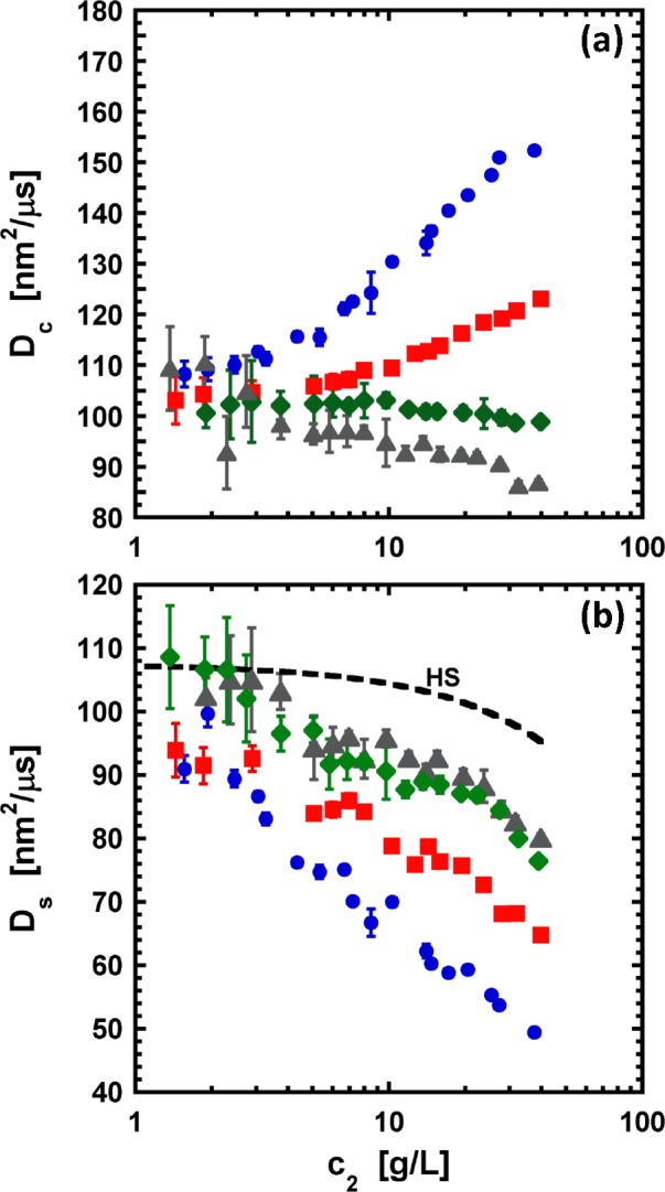
Values of the collective (or mutual) diffusion coefficient D_c (panel a) and the self-diffusion coefficient D_s (panel b) as a function of protein concentration for α-chymotrypsinogen. Symbols correspond to the different salt concentrations: (circles) 0; (squares) 10; (diamonds) 50; and (triangles) 100 mM. D_s was calculated from combining D_c with R₉₀/K (cf. Figure 1) via eq 9. The dashed line in panel b corresponds to the theoretical D_s for a system of suspended hard spheres 4 nm in diameter.

Table 1. Interaction Parameter k_D and Osmotic Second Virial Coefficient B₂₂ for aCgn at Different NaCl Concentrations.

NaCl [mM]	B22 [mL/g]	kD [mL/g]
0	52 ± 6	24 ± 3
10	22 ± 4	4.4 ± 1.6
50	5.8 ± 3.8	–2.9 ± 2.2
100	3 ± 3	–12.5 ± 8.6

Qualitatively, the behavior of k_D is equivalent to that displayed by B₂₂ in that increases of salt concentration give rise to a significant decrease of the strength of protein repulsions. However, values of k_D at high salt concentration indicate that there are net attractive protein interactions, which appears to contradict the results obtained from SLS and SANS. By plotting B₂₂ versus k_D (see the Supporting Information), one can see that k_D scales linearly with B₂₂, but the intercept is smaller than 0. On the basis of eq 10, hydrodynamic interactions may also play a significant role on the behavior of D_c, and thus, the discrepancies observed here between k_D and B₂₂ are perhaps not surprising, but they suggest that the contribution from hydrodynamic interactions is relevant in the behavior of aCgn.

Figure 6 illustrates the competition between protein–protein and hydrodynamic interactions, as well as the effect of the range of protein–protein interactions on the mobility of proteins in solution. At high salt concentration (short interaction range), the diffusion of proteins is dominated by hydrodynamic interactions as S(q → 0) ≈ 1 (see Figure 5). In contrast, at low salt concentrations, both S(q → 0) and H(q → 0) are large, but the structure factor represents the major contribution to D_c, leading to increase D_c as the protein concentration increases. Overall, the contribution from H(q → 0) is appreciable for all of the conditions tested here.

Discussion

Three different experimental methods to probe concentration-dependent protein–protein interactions were tested here: SLS, SANS, and DLS. The first two techniques allow one to assess the “direct” or thermodynamic interactions either in the q → 0 limit (via B₂₂ or G₂₂ from SLS) or as a function of the wave vector (via I(Q) from SANS). The results in Figures 2a, 3, and 4 show that the qualitative behavior of protein interactions for aCgn with respect to solution conditions (i.e., changes in salt concentration) is captured by both SLS and SANS. This behavior indicates that intermolecular interactions are dominated by electrostatic forces in that strong repulsive forces are exhibited at low NaCl concentration, and the strength of these interactions decreases as the salt concentration increases. Similarly, the results also show that the strength of the repulsions also decreases as a consequence of increasing protein concentration (e.g., G₂₂ versus c₂ in Figure 3). While the effect of NaCl concentration on protein–protein interactions can be intuitively attributed to screening effects as a consequence of accumulation of ions on the protein surface,⁹⁷ the behavior of these interactions with respect to protein concentration may be due to more complex effects. Although molecular crowding, self-buffering, and non-negligible concentrations of counterions may affect the strength of protein–protein interactions at concentrated conditions,^98,99 none of these effects alone can explain the observed qualitative behavior of protein interactions versus protein concentration at the moderate range of concentrations tested here (see the discussion below).

On the other hand, DLS experiments provide information from both direct protein interactions and hydrodynamic interactions via D_c, D_s, or k_D. The results in Figure 5 and Table 1 show that both types of interactions play a major role in the DLS behavior of aCgn at the conditions tested here. At low protein concentrations, differences in the sign of the interaction parameter k_D and B₂₂ (cf. Table 1) indicate a major effect from hydrodynamic interactions. Indeed, comparison of eqs 8 and 10 illustrates that for conditions where hydrodynamic interactions are non-negligible with respect to the evaluated range of protein concentrations (i.e., h₁ ≠ 0), k_D may be a poor representation of thermodynamic protein interactions. The convolution of both types of interactions on the behavior of aCgn in solution is even more evident at high protein concentration. Although eq 9 suggests that thermodynamic contributions to the net protein–protein interactions primarily affect D_c through S(q → 0), the results in Figure 6 show that D_s is sensitive to salt concentration, which is unexpected if all effects of direct protein–protein interaction on D_c are captured by the structure factor. However, the hydrodynamic factor (H(q)) also implicitly considers the effect of these interactions on the mobility of proteins, in that intermolecular interactions dictate the forces that affect how neighboring proteins move, and therefore affect the local hydrodynamic field. That is, stronger repulsive (attractive) protein interactions, with respect to a noninteracting system (e.g., a hard-sphere system), lead to stronger (weaker) hydrodynamic interactions.

Felderhof¹⁰⁰ showed that by using a Taylor expansion in terms of the inverse of the center-to-center distance, one can approximate the hydrodynamic factor as a linear function of c₂, where the slope depends on the effect of the PMF on the different hydrodynamic forces (i.e., hydrodynamic dipole, short-range and self-contributions). Similarly, more elaborate approximations have been developed to incorporate the effect of thermodynamic contributions on D_c via pairwise additivity assumptions¹⁰¹ or decomposition of H(q → 0) into direct and indirect terms.¹⁰² Although such approximations are shown to be accurate only at dilute conditions,^81,103,104 it illustrates how direct protein interactions can be expected to play a role in the hydrodynamics of protein solutions.

Additionally, the analysis here allows one to test a common practice in characterizing net protein–protein interactions: the use of simplified PMF models to represent these interactions. Although such models may provide a valuable way to infer some information about the underlying interactions of the system (e.g., consider the SANS data in Figure 5, where reaching Q → 0 is not practical without extrapolating with the aid of a PMF model), one needs to be careful in interpreting the results from these models. As discussed above, the PMF is an ensemble-averaged quantity that is an implicit function of the solution conditions (pH, c₂, concentration of cosolutes, temperature), and therefore, one may anticipate that different PMFs are required at different conditions (cf. Figure 4). On the basis of colloidal science arguments, protein–protein PMFs in solution are due to at least three main contributions, sterics or excluded volume (e.g., a hard-sphere-like potential), short-range attractions due to dispersion forces and solvophobic interactions, and screened electrostatic repulsions/attractions. Short-range attractions are strong interactions with an effective range of a few Angströms. The net magnitude of these contributions may be expected to change with temperature or c₂ but shows little to no change with ionic strength and pH within the range of conditions here.^97,105

By contrast, electrostatic interactions are long-ranged in nature, where the strength and the range of these interactions is sensitive to the conditions of the medium (pH, dielectric constant, ionic strength). At dilute protein conditions, the maximum effective range of the interactions between charged moieties is expected to range from 5 to 10 nm (for ionic strengths of ∼10 mM) to a few Angströms (for ionic strengths of ∼500 mM).^97,105 Similarly, if one considers that the protein net charge is the result of the sum of the charges of all titratable side chains that have no greater charge than ±1, the effective strength (or effective “charge”) of screened electrostatic interactions at low ionic strengths is no greater than that for short-range attractions at near-contact between amino acids side chains with center-to-center distances of ∼5 Å. Furthermore, one may anticipate that the protein net charge may diminish at high salt concentrations as a result of ion condensation effects.^105,106 At high protein concentration, electrostatic interactions may also be affected by other factors such as polarizability, self-buffering, and condensation of ions at the protein surface as a consequence of a non-negligible concentration of counterions in solution^98,99 (e.g., for aCgn at pH 3.5, in order to maintain electroneutrality, the number of counterion molecules in solution is at least an order of magnitude larger than that of the protein).

Therefore, for fitted PMFs to be considered physically meaningful, they should at least be able to represent the qualitative behavior of protein–protein interactions with changes in solution conditions. The above analysis and results show that this qualitative behavior is not fully captured with the PMF models tested here. Although fits to these PMFs at a given solution condition do not provide a reason to be suspect from a statistical standpoint (e.g., fits appear reasonable in Figure 4), the results from neither SLS nor SANS data were able to provide physically reasonable trends for the effective strength and range of the different types of forces (i.e., short-range attractions, electrostatics interactions) as a function of protein or cosolute concentration. This may be problematic as the “true” PMF is never known a priori for any experimental system and can only be experimentally assessed from fully converged SAXS or SANS intensity profiles of proteins with simple geometries at moderate to high c₂, where S(Q) is the dominant factor if the form factor does not change with protein concentration. This poses additional limitations in terms of the time required to collect data (unless one is at rather high c₂) as well as regular access to a neutron or X-ray synchrotron facility, which is problematic for applications such as biotechnology product development. If one does not require the spatial information contained within a SANS or SAXS profile, then the local Taylor series approach to determine G₂₂ is a convenient experimental means to quantify the thermodynamics and net interactions of protein solutions as a function of protein concentration and solvent conditions.

Despite the issues noted above for determining a robust and quantitative PMF for protein–protein interactions, one may still quantify the net interactions and the thermodynamic nonidealities without the need for a PMF. G₂₂ is potentially advantageous in this regard because it provides a rigorous and quantitative relation between multibody protein interactions and the thermodynamics of proteins in solution.^59,107G₂₂, as well as other KB integrals, is related to changes in different thermodynamic variables such as the isothermal compressibility or partial molar or specific volumes.^47,72 In the case of G₂₂, changes in the protein chemical potential are given by^108,107

12

where R is the ideal gas constant, T is the absolute temperature, V is the system volume, and μ₂ is the protein chemical potential. Note that the subscript in the derivative indicates that it is taken at fixed T, V, and chemical potentials of all of the species in the solution other than that of the protein (μ′). In this regard, this derivative describes an implicit solvent system such as those observed from osmometry experiments and described by McMillan–Mayer theory.^47,109 Thus, direct integration of R₉₀ via eq 12 should be avoided if one is seeking to integrate along a path of fixed temperature, pressure (p), and cosolute concentration (c₃). While the set of scattering measurements are commonly performed along a series of c₂ values for a common (T,p,c₃) pathway, the derivative of μ₂ obtained from LS is not at fixed (T,p,c₃). As a result, it is not straightforward to obtain derivatives of activity coefficients for proteins or cosolutes from only LS data alone,^47,59,68,69 and doing so therefore requires additional analysis if one seeks to relate LS to the location of phase boundaries.^34,110 A similar issue arises if one attempts to relate the integrated μ₂ versus c₂ to the PMF⁴⁸ as the solvent and solute chemical potentials change as a function of c₂.

These issues can potentially be avoided by alternative sample preparation in order to maintain an equal chemical potential of (co)solvent and cosolutes at all protein concentrations. For instance, by exhaustively dialyzing each protein sample against the same solvent (e.g., buffer plus cosolutes), the chemical potential of all of the other species will be constant and equal to that of the solvent, and one can correctly integrate the partial derivative in eq 12 versus c₂ to recover μ₂ as a function of c₂. However, this requires that one perform a separate dialysis preparation for each c₂ value, independently, for a given salt concentration. Doing so is not common practice as it is typically not logistically practical due to the greatly increased requirements of time, protein material, and/or cost to prepare a large number of samples with different protein concentrations in this manner.

Alternatively, one can consider the behavior of G₂₂ from a statistical-thermodynamic standpoint. As eq 5 shows, G₂₂ is related to the integral over g̅₂₂(r), and thus, it indirectly allows one to assess local changes in composition around a given protein molecule (i.e., the region where g̅₂₂(r) ≠ 1).⁴⁷ That is, G₂₂ depends on the local variations of concentration with respect to the bulk concentration. Likewise, G₂₂ and eq 12 qualitatively and semiquantitatively relate the local fluctuations in protein concentration to the thermodynamic behavior of proteins in solution because 1 + c₂G₂₂ is proportional to the magnitude and sign of local fluctuations in protein concentration.^47,72 Positive (negative) deviations from zero for c₂G₂₂ indicate large (small) variations in the local density of proteins with respect to an ideal gas mixture.^107,108 Notably, there is a strict lower bound for the product of c₂G₂₂ based on thermodynamic stability criteria as c₂G₂₂ less than or equal to −1 violates stability criteria.¹¹¹ While there is no rigorous upper bound for c₂G₂₂ (i.e., strongly attractive conditions), c₂G₂₂ ≫ 1 is indicative of being in proximity to homogeneous transitions (e.g., fluid–fluid phase separation or critical opalescence). Such processes yield extremely large molecular fluctuations as a consequence of long-range density and composition fluctuations as one approaches a spinodal.

To a first approximation, when G₂₂ (in units of volume per mole of protein) is negative, then its magnitude is effectively the excluded volume that the other proteins “feel” from a central protein; similarly, 1 + c₂G₂₂ then represents the effective “free” volume fraction (i.e., the volume that is not excluded by proteins) of the system under repulsive conditions. This is also consistent with it being physically impossible to achieve c₂G₂₂ less than −1 for an equilibrium system. In contrast, for positive G₂₂ there is no simple excluded volume analogy because excluded volume is positive by definition. In that case, c₂G₂₂ physically represents the extent of statistical accumulation of protein (relative to solvent/cosolutes) in the near-neighbor shells compared to what one would have for ideal solutions.⁴⁷ If one makes the assumption that g̅₂₂(r) is only short-ranged when G₂₂ is positive (attractive conditions), then c₂G₂₂ roughly represents the average number of nearest-neighbor proteins in the grand-canonical ensemble. As all of the conditions investigated here showed negative G₂₂ values, the former physical picture holds. As 1 + c₂G₂₂ decreases, this indicates a decrease in the effective volume fraction that remains for other proteins to be added to the system as c₂ is increased to larger values (Figure 5). If one were to simply define the effective protein excluded volume fraction (ϕ_eff = c₂B₂^HS) based on the excluded volume of protein at infinite dilution, the largest free volume fraction (=1 – ϕ_eff) that one would reach is ∼0.89 at 35 g/L. Comparison with Figure 5 shows that this is a gross underestimation of ϕ_eff when long-ranged repulsions are present. A similar conclusion can be drawn if one considers the effective “hard-sphere” diameter (σ_eff) that yields the same value of S(q → 0) or c₂G₂₂ at a given protein concentration via a hard-sphere equation of state such as the Carnahan–Starling approximation¹¹² (data not shown). For instance, at no added NaCl, when electrostatic repulsions are the strongest, σ_eff is ∼10 nm (i.e., ∼2.5 times larger than the protein diameter) at low protein concentrations and decreases to ∼7 nm at 20 g/L of protein as a consequence of the decrease on the strength of the repulsions due to thermodynamic nonidealities.

This change in the effective protein excluded volume or effective protein diameter with protein interactions and c₂ might suggest that the behavior of aCgn solutions, at repulsive conditions, is effectively equivalent to that of a system experiencing molecular crowding, even though the volume fraction based on just the protein molecular volume is far below that where large effects due to crowding are expected for a hard-sphere system. This observation is consistent with the qualitative behavior of the hydrodynamic factor with respect to protein concentration. Strong hydrodynamic interactions have typically been associated with molecular crowding, and thus, they are only considered important on systems where protein and/or cosolute concentrations are large.^13,113−115 Furthermore, when hydrodynamic interactions are considered, H(q → 0) versus c₂ is typically treated via simple relations, which assume in most cases that H(q → 0) is linear with respect to protein concentration.^81,100 However, as Figure 6b shows, the hydrodynamic contribution as a function of protein concentration is neither simple nor negligible at even these low concentrations (i.e., less than 5 w/v%). Comparison of experimental D_s values (Figure 6) with those of a hard-sphere system shows that hydrodynamic interactions are more complex than simple steric effects (i.e., based on molecular volume alone). The results in Figure 6b also suggest that the range of electrostatic interactions plays a key role in the strength of hydrodynamic interactions, with low (high) salt concentration leading to stronger (weaker) hydrodynamic interactions. Such effects may be the result of an increase in the effective excluded protein volume as the range of charge–charge interactions increases, similar to the case of G₂₂. Quantitatively, the reduction on D_s from D₀ observed here lies between 20 (for 100 mM NaCl) and 50% (for 0 mM NaCl) at a protein concentration of 40 g/L. Although similar effects of the range of electrostatic interaction on the self-diffusion of proteins have been observed previously,^{80,81,115−117} they have been found for protein volume fractions > 10%, which would correspond to c₂ > 120 g/L for a protein of the size of aCgn.

Summary and Conclusions

Protein interactions as a function of protein and salt concentration were evaluated via scattering methods (SLS, SANS, and DLS) for solutions of monomeric α-chymotrypsinogen at acidic pH. Equilibrium net protein–protein interactions were assessed via the protein–protein KB integral G₂₂ and the structure factor S(Q) from SLS and SANS data, respectively. G₂₂ was obtained by regressing the Rayleigh ratio versus protein concentration to eq 4 using a local Taylor series approach, which allows one to quantify interactions without biasing the results toward a specific model for intermolecular interactions (i.e., PMF models). G₂₂ versus c₂ curves, as well as SANS intensity spectra I(Q), were further analyzed via traditional methods involving fits to effective intermolecular potentials (i.e., PMF models). These fits were able to capture the curves of G₂₂ or I(Q) as long as one considered concentration-dependent model parameters and accepted that the fitted parameters showed unphysical trends in some cases. The values of S(Q → 0) from SLS and from extrapolating SANS data to Q → 0 were quantitatively consistent.

In the dilute regime, fitted G₂₂ values agreed with those obtained via the osmotic second virial coefficient (B₂₂) and showed that electrostatic interactions dominated the scattering behavior for aCgn under these pH and salt conditions. However, as the protein concentration increased, the magnitude of the protein–protein repulsions decreased, with a more pronounced effect for those conditions where B₂₂ was larger. Both SLS and SANS results indicated that the thermodynamic behavior of the aCgn solution is similar to that observed in systems under molecular crowding, despite the moderate range of protein concentrations used here (c₂ < 40 g/L). As was anticipated in a previous study,⁵⁹ both the strength and the range of protein–protein interactions modulate this crowding-like effect, such that strong and long-range protein interactions led to more noticeable thermodynamic nonidealities.

The zero-q limit hydrodynamic factor H(q → 0) (or alternatively the self-diffusion coefficient D_s) was also assessed to quantify hydrodynamic nonidealities by combining measurements of the collective diffusion coefficient (D_c) from DLS data with measurements of S(q → 0) via eq 9. Curves of D_c versus c₂ illustrated the competition between equilibrium protein interactions (probed via G₂₂) and hydrodynamic interactions as a consequence of the range of intermolecular interactions. While at high salt concentrations H(q → 0) is the dominant contribution to D_c, at low salt concentration, the net mobility of proteins is dictated by S(q → 0). Nevertheless, the hydrodynamic contribution was found to be significant for all of the conditions and correlated with the strength of colloidal interactions such that larger repulsive B₂₂ values correspond to stronger hydrodynamic interactions. Quantitatively, the reduction of D_s due to increased protein concentration was much larger than what could be expected based on purely steric interactions, highlighting that the long-range repulsions resulted in a much larger effective excluded volume contribution to protein–protein interactions probed by S(q → 0) and by H(q → 0).

Supporting Information Available

Details regarding the implementation of the local Taylor series approach to obtain G₂₂ as well as a statistical analysis of this method are provided. Additionally, a general overview of the static structure factor and G₂₂ for the different PMF models is considered, including the resulting fitted parameter from regressing these models to the experimental data of I(Q) and G₂₂. This material is available free of charge via the Internet at http://pubs.acs.org.

The authors declare no competing financial interest.

Funding Statement

National Institutes of Health, United States

References

- Gavin A. C.; Bosche M.; Krause R.; Grandi P.; Marzioch M.; Bauer A.; Schultz J.; Rick J. M.; Michon A. M.; Cruciat C. M.; et al. Functional Organization of the Yeast Proteome by Systematic Analysis of Protein Complexes. Nature 2002, 415, 141–147. [DOI] [PubMed] [Google Scholar]
- Williams D. H.; Stephens E.; O’Brien D. P.; Zhou M. Understanding Noncovalent Interactions: Ligand Binding Energy and Catalytic Efficiency from Ligand-Induced Reductions in Motion within Receptors and Enzymes. Angew. Chem. 2004, 43, 6596–6616. [DOI] [PubMed] [Google Scholar]
- Pawson T. Specificity in Signal Transduction: From Phosphotyrosine–SH2 Domain Interactions to Complex Cellular Systems. Cell 2004, 116, 191–203. [DOI] [PubMed] [Google Scholar]
- Carroll M. C. The Complement System in Regulation of Adaptive Immunity. Nat. Immunol. 2004, 5, 981–986. [DOI] [PubMed] [Google Scholar]
- Wang W. Protein Aggregation and Its Inhibition in Biopharmaceutics. Int. J. Pharm. 2005, 289, 1–30. [DOI] [PubMed] [Google Scholar]
- Roberts C. J. Non-Native Protein Aggregation Kinetics. Biotechnol. Bioeng. 2007, 98, 927–938. [DOI] [PubMed] [Google Scholar]
- Saluja A.; Kalonia D. S. Nature and Consequences of Protein–Protein Interactions in High Protein Concentration Solutions. Int. J. Pharm. 2008, 358, 1–15. [DOI] [PubMed] [Google Scholar]
- Weiss W. F. IV; Young T. M.; Roberts C. J. Principles, Approaches, and Challenges for Predicting Protein Aggregation Rates and Shelf Life. J. Pharm. Sci. 2009, 98, 1246–1277. [DOI] [PubMed] [Google Scholar]
- Lewus R. A.; Darcy P. A.; Lenhoff A. M.; Sandler S. I. Interactions and Phase Behavior of a Monoclonal Antibody. Biotechnol. Prog. 2011, 27, 280–289. [DOI] [PubMed] [Google Scholar]
- Mason B. D.; Zhang L.; Remmele R. L. Jr.; Zhang J. Opalescence of an IgG2 Monoclonal Antibody Solution as it Relates to Liquid–Liquid Phase Separation. J. Pharm. Sci. 2011, 100, 4587–4596. [DOI] [PubMed] [Google Scholar]
- Silverman L.; Glick D. Measurement of Protein Concentration by Quantitative Electron Microscopy. J. Cell Biol. 1969, 40, 773. [DOI] [PMC free article] [PubMed] [Google Scholar]
- Kentsis A.; Gordon R. E.; Borden K. L. B. Control of Biochemical Reactions Through Supramolecular RING Domain Self-Assembly. Proc. Natl. Acad. Sci. U.S.A. 2002, 99, 15404–15409. [DOI] [PMC free article] [PubMed] [Google Scholar]
- Sun J.; Weinstein H. Toward Realistic Modeling of Dynamic Processes in Cell Signaling: Quantification of Macromolecular Crowding Effects. J. Chem. Phys. 2007, 127, 155105. [DOI] [PubMed] [Google Scholar]
- Du F.; Zhou Z.; Mo Z.-Y.; Shi J.-Z.; Chen J.; Liang Y. Mixed Macromolecular Crowding Accelerates the Refolding of Rabbit Muscle Creatine Kinase: Implications for Protein Folding in Physiological Environments. J. Mol. Biol. 2006, 364, 469–482. [DOI] [PubMed] [Google Scholar]
- Ross C. A.; Tabrizi S. J. Huntington’s Disease: From Molecular Pathogenesis to Clinical Treatment. Lancet Neurol. 2011, 10, 83–98. [DOI] [PubMed] [Google Scholar]
- Dobson C. M. Principles of Protein Folding, Misfolding and Aggregation. Semin. Cell Dev. Biol. 2004, 15, 3–16. [DOI] [PubMed] [Google Scholar]
- Moreau K. L.; King J. A. Protein Misfolding and Aggregation in Cataract Disease and Prospects for Prevention. Trends Mol. Med. 2012, 18, 273–282. [DOI] [PMC free article] [PubMed] [Google Scholar]
- Schuck P. Use of Surface Plasmon Resonance to Probe the Equilibrium and Dynamic Aspects of Interactions between Biological Macromolecules. Annu. Rev. Biophys. Biomol. Struct. 1997, 26, 541–566. [DOI] [PubMed] [Google Scholar]
- Joo C.; Balci H.; Ishitsuka Y.; Buranachai C.; Ha T. Advances in Single-Molecule Fluorescence Methods for Molecular Biology. Annu. Rev. Biochem. 2008, 77, 51–76. [DOI] [PubMed] [Google Scholar]
- Veraksa A.; Bauer A.; Artavanis-Tsakonas S. Analyzing Protein Complexes in Drosophila with Tandem Affinity Purification-Mass Spectrometry. Dev. Dyn. 2005, 232, 827–834. [DOI] [PubMed] [Google Scholar]
- Ali M. H.; Imperiali B. Protein Oligomerization: How and Why. Bioorg. Med. Chem. 2005, 13, 5013–5020. [DOI] [PubMed] [Google Scholar]
- Moon Y. U.; Curtis R. A.; Anderson C. O.; Blanch H. W.; Prausnitz J. M. Protein–Protein Interactions in Aqueous Ammonium Sulfate Solutions. Lysozyme and Bovine Serum Albumin (BSA). J. Solution Chem. 2000, 29, 699–717. [Google Scholar]
- Liu J.; Nguyen M. D. H.; Andya J. D.; Shire S. J. Reversible Self-Association Increases the Viscosity of a Concentrated Monoclonal Antibody in Aqueous Solution. J. Pharm. Sci. 2005, 94, 1928–1940. [DOI] [PubMed] [Google Scholar]
- Saluja A.; Badkar A. V.; Zeng D. L.; Nema S.; Kalonia D. S. Ultrasonic Storage Modulus as a Novel Parameter for Analyzing Protein–Protein Interactions in High Protein Concentration Solutions: Correlation with Static and Dynamic Light Scattering Measurements. Biophys. J. 2007, 92, 234–244. [DOI] [PMC free article] [PubMed] [Google Scholar]
- Perez J. M.; Josephson L.; O’Loughlin T.; Hogemann D.; Weissleder R. Magnetic Relaxation Switches Capable of Sensing Molecular Interactions. Nat. Biotechnol. 2002, 20, 816–820. [DOI] [PubMed] [Google Scholar]
- Scherer T. M.; Liu J.; Shire S. J.; Minton A. I. Intermolecular Interactions of IgG1Monoclonal Antibodies at High Concentrations Characterized by Light Scattering. J. Phys. Chem. B 2010, 114, 12948–12957. [DOI] [PubMed] [Google Scholar]
- Narayanan J.; Liu X. Y. Protein Interactions in Undersaturated and Supersaturated Solutions: A Study Using Light and X-ray Scattering. Biophys. J. 2003, 84, 523–532. [DOI] [PMC free article] [PubMed] [Google Scholar]
- Shukla A.; Mylonas E.; Di Cola E.; Finet S.; Timmins P.; Narayanan T.; Svergun D. I. Absence of Equilibrium Cluster Phase in Concentrated Lysozyme Solutions. Proc. Natl. Acad. Sci. U.S.A. 2008, 105, 5075–5080. [DOI] [PMC free article] [PubMed] [Google Scholar]
- Guo B.; Kao S.; McDonald H.; Asanov A.; Combs L. L.; Wilson W. W. Correlation of Second Virial Coefficients and Solubilities Useful in Protein Crystal Growth. J. Cryst. Growth 1999, 196, 424–433. [Google Scholar]
- Dumetz A. C.; Snellinger-O’Brien A. M.; Kaler E. W.; Lenhoff A. M. Patterns of Protein–Protein Interactions in Salt Solutions and Implications for Protein Crystallization. Protein Sci. 2007, 16, 1867–1877. [DOI] [PMC free article] [PubMed] [Google Scholar]
- Saluja A.; Fesinmeyer R. M.; Hogan S.; Brems D. N.; Gokarn Y. R. Diffusion and Sedimentation Interaction Parameters for Measuring the Second Virial Coefficient and Their Utility as Predictors of Protein Aggregation. Biophys. J. 2010, 99, 2657–2665. [DOI] [PMC free article] [PubMed] [Google Scholar]
- Petsev D. N.; Wu X. X.; Galkin O.; Vekilov P. G. Thermodynamic Functions of Concentrated Protein Solutions from Phase Equilibria. J. Phys. Chem. B 2003, 107, 3921–3926. [Google Scholar]
- Carrotta R.; Manno M.; Giordano F. M.; Longo A.; Portale G.; Martorana V.; Biagio P. L. S. Protein Stability Modulated by a Conformational Effector: Effects of Trifluoroethanol on Bovine Serum Albumin. Phys. Chem. Chem. Phys. 2009, 11, 4007–4018. [DOI] [PubMed] [Google Scholar]
- Curtis R. A.; Blanch H. W.; Prausnitz J. M. Calculation of Phase Diagrams for Aqueous Protein Solutions. J. Phys. Chem. B 2001, 105, 2445–2452. [Google Scholar]
- Li Y.; Ogunnaike B. A.; Roberts C. J. Multi-Variate Approach to Global Protein Aggregation Behavior and Kinetics: Effects of pH, NaCl, and Temperature for α-Chymotrypsinogen A. J. Pharm. Sci. 2010, 99, 645–662. [DOI] [PubMed] [Google Scholar]
- Tessier P. M.; Lenhoff A. M.; Sandler S. I. Rapid Measurement of Protein Osmotic Second Virial Coefficients by Self-Interaction Chromatography. Biophys. J. 2002, 82, 1620–1631. [DOI] [PMC free article] [PubMed] [Google Scholar]
- Orellana C. A.; Shene C.; Asenjo J. A. Mathematical Modeling of Elution Curves for a Protein Mixture in Ion Exchange Chromatography Applied to High Protein Concentration. Biotechnol. Bioeng. 2009, 104, 572–581. [DOI] [PubMed] [Google Scholar]
- Winzor D. J.; Deszczynski M.; Harding S. E.; Wills P. R. Nonequivalence of Second Virial Coefficients from Sedimentation Equilibrium and Static Light Scattering Studies of Protein Solutions. Biophys. Chem. 2007, 128, 46–55. [DOI] [PubMed] [Google Scholar]
- Neergaard M. S.; Kalonia D. S.; Parshad H.; Nielsen A. D.; Möller E. H.; van de Weert M. Viscosity of High Concentration Protein Formulations of Monoclonal Antibodies of the IgG1 and IgG4 Subclass: Prediction of Viscosity through Protein–Protein Interaction Measurements. Eur. J. Pharm. Sci. 2013, 49, 400–410. [DOI] [PubMed] [Google Scholar]
- Yadav S.; Scherer T. M.; Shire S. J.; Kalonia D. S. Use of Dynamic Light Scattering to Determine Second Virial Coefficient in a Semidilute Concentration Regime. Anal. Biochem. 2011, 411, 292–296. [DOI] [PubMed] [Google Scholar]
- Rosenbaum D. F.; Zukoski C. F. Protein Interactions and Crystallization. J. Cryst. Growth 1996, 169, 752–758. [Google Scholar]
- Neal B. L.; Asthagiri D.; Velev O. D.; Lenhoff A. M.; Kaler E. W. Why is the Osmotic Second Virial Coefficient Related to Protein Crystallization?. J. Cryst. Growth 1999, 196, 377–387. [Google Scholar]
- Schaink H. M.; Smit J. A. M. Determination of the Osmotic Second Virial Coefficient and the Dimerization of β-Lactoglobulin in Aqueous Solutions with Added Salt at the Isoelectric Point. Phys. Chem. Chem. Phys. 2000, 2, 1537–1541. [Google Scholar]
- Zhang J.; Liu X. Y. Effect of Protein–Protein Interactions on Protein Aggregation Kinetics. J. Chem. Phys. 2003, 119, 10972–10976. [Google Scholar]
- Chari R.; Jerath K.; Badkar A. V.; Kalonia D. S. Long- and Short-Range Electrostatic Interactions Affect the Rheology of Highly Concentrated Antibody Solutions. Pharm. Res. 2009, 26, 2607–2618. [DOI] [PubMed] [Google Scholar]
- Zhou H.-X. Influence of Crowded Cellular Environments on Protein Folding, Binding, and Oligomerization: Biological Consequences and Potentials of Atomistic Modeling. FEBS Lett. 2013, 587, 1053–1061. [DOI] [PMC free article] [PubMed] [Google Scholar]
- Ben-Naim A.Statistical Thermodynamics for Chemists and Biochemists; Plenum Press: New York, 1992. [Google Scholar]
- Scherer T. M. Cosolute Effects on the Chemical Potential and Interactions of an IgG1Monoclonal Antibody at High Concentrations. J. Phys. Chem. B 2013, 117, 2254–2266. [DOI] [PubMed] [Google Scholar]
- Minton A. P. Static Light Scattering from Concentrated Protein Solutions, I: General Theory for Protein Mixtures and Application to Self-Associating Proteins. Biophys. J. 2007, 93, 1321–1328. [DOI] [PMC free article] [PubMed] [Google Scholar]
- Posharnowa N.; Schneider A.; Wunsch M.; Kuleznew V.; Wolf B. A. Polymer–Polymer Interaction Parameters for Homopolymers and Copolymers from Light Scattering and Phase Separation Experiments in a Common Solvent. J. Chem. Phys. 2001, 115, 9536–9546. [Google Scholar]
- Schartl W.Light Scattering from Polymer Solutions and Nanoparticle Dispersions; Springer-Verlag: Berlin and Heidelberg, Germany, New York, 2007. [Google Scholar]
- Rojas-Ochoa L. F.; Castaneda-Priego R.; Lobaskin V.; Stradner A.; Scheffold F.; Schurtenberger P. Density Dependent Interactions and Structure of Charged Colloidal Dispersions in the Weak Screening Regime. Phys. Rev. Lett. 2008, 100, 178304. [DOI] [PubMed] [Google Scholar]
- Fernandez C.; Minton A. P. Automated Measurement of the Static Light Scattering of Macromolecular Solutions over a Broad Range of Concentrations. Anal. Biochem. 2008, 381, 254–257. [DOI] [PMC free article] [PubMed] [Google Scholar]
- Lindner P.; Zemb T.. Neutrons, X-rays and Light: Scattering Methods Applied to Soft Condensed Matter; Elsevier Science B.V.: Amsterdam, The Netherlands, 2002. [Google Scholar]
- Brumberger H.Modern Aspects of Small-Angle Scattering; NATO ASI Series. Ser. C: Mathematical and Physical Sciences; Springer: Dordrecht, The Netherlands, 1995. [Google Scholar]
- Zhang F.; Skoda M. W. A.; Jacobs R. M. J.; Martin R. A.; Martin C. M.; Schreiber F. Protein Interactions Studied by SAXS: Effect of Ionic Strength and Protein Concentration for BSA in Aqueous Solutions. J. Phys. Chem. B 2007, 111, 251–259. [DOI] [PubMed] [Google Scholar]
- Jin L.; Yu Y.-X.; Gao G.-H. A Molecular-Thermodynamic Model for the Interactions Between Globular Proteins in Aqueous Solutions: Applications to Bovine Serum Albumin (BSA), Lysozyme, α-Chymotrypsin, and Immuno-Gamma-Globulins (IgG) Solutions. J. Colloid Interface Sci. 2006, 304, 77–83. [DOI] [PubMed] [Google Scholar]
- Niebuhr M.; Koch M. H. J. Effects of Urea and Trimethylamine-N-Oxide (TMAO) on the Interactions of Lysozyme in Solution. Biophys. J. 2005, 89, 1978–1983. [DOI] [PMC free article] [PubMed] [Google Scholar]
- Blanco M. A.; Sahin E.; Li Y.; Roberts C. J. Reexamining Protein–Protein and Protein–Solvent Interactions from Kirkwood–Buff Analysis of Light Scattering in Multi-Component Solutions. J. Chem. Phys. 2011, 134, 225103. [DOI] [PMC free article] [PubMed] [Google Scholar]
- Andrews J. M.; Weiss W. F.; Roberts C. J. Nucleation, Growth, and Activation Energies for Seeded and Unseeded Aggregation of α-Chymotrypsinogen A. Biochemistry 2008, 47, 2397–2403. [DOI] [PubMed] [Google Scholar]
- Velev O. D.; Kaler E. W.; Lenhoff A. M. Protein Interactions in Solution Characterized by Light and Neutron Scattering: Comparison of Lysozyme and Chymotrypsinogen. Biophys. J. 1998, 75, 2682–2697. [DOI] [PMC free article] [PubMed] [Google Scholar]
- Weiss W. F. IV; Hodgdon T. K.; Kaler E. W.; Lenhoff A. M.; Roberts C. J. Nonnative Protein Polymers: Structure, Morphology, and Relation to Nucleation and Growth. Biophys. J. 2007, 93, 4392–4403. [DOI] [PMC free article] [PubMed] [Google Scholar]
- Weiss W. F. IV; Zhang A.; Ivanova M. A.; Sahin E.; Jordan J. L.; Fernandez E. J.; Roberts C. J. Reduction of the C191-C220 Disulfide of α-Chymotrypsinogen A Accelerates Amyloid Formation via Reduced Nucleation Barriers. Biophys. Chem. 2014, 185, 79–87. [DOI] [PMC free article] [PubMed] [Google Scholar]
- Glasoe P. K.; Long F. A. Use of Glass Electrodes to Measure Acidities in Deuterium Oxide. J. Phys. Chem. 1960, 64, 188–190. [Google Scholar]
- Brummitt R. K.; Andrews J. M.; Jordan J. L.; Fernandez E. J.; Roberts C. J. Thermodynamics of Amyloid Dissociation Provide Insights into Aggregate Stability Regimes. Biophys. Chem. 2012, 168, 10–18. [DOI] [PubMed] [Google Scholar]
- Hiemenz P. C.; Rajagopalan R.. Principles of Colloid and Surface Chemistry, 3rd ed.; Marcel Dekker Inc.: New York, 1997. [Google Scholar]
- Raccosta S.; Martorana V.; Manno M. Thermodynamic versus Conformational Metastability in Fibril-Forming Lysozyme Solutions. J. Phys. Chem. B 2012, 116, 12078–12087. [DOI] [PubMed] [Google Scholar]
- Stockmayer W. H. Light Scattering in Multi-Component Systems. J. Chem. Phys. 1950, 18, 58–61. [Google Scholar]
- Kirkwood J. G.; Goldenberg R. J. Light Scattering Arising from Composition Fluctuations in Multi-Component Systems. J. Chem. Phys. 1950, 18, 54–57. [Google Scholar]
- Zimm B. H. Apparatus and Methods for Measurement and Interpretation of the Angular Variation of Light Scattering — Preliminary Results on Polystyrene Solutions. J. Chem. Phys. 1948, 16, 1099–1116. [Google Scholar]
- Zimm B. H. The Scattering of Light and the Radial Distribution Function of High Polymer Solutions. J. Chem. Phys. 1948, 16, 1093–1099. [Google Scholar]
- Kirkwood J. G.; Buff F. P. The Statistical Mechanical Theory of Solutions. 1. J. Chem. Phys. 1951, 19, 774–777. [Google Scholar]
- Berne B. J.; Pecora R.. Dynamic Light Scattering: With Applications to Chemistry, Biology, and Physics; Wiley: New York, 1976. [Google Scholar]
- Frisken B. Revisiting the Method of Cumulants for the Analysis of Dynamic Light-Scattering Data. Appl. Opt. 2001, 40, 4087–4091. [DOI] [PubMed] [Google Scholar]
- Koppel D. E. Analysis of Macromolecular Polydispersity in Intensity Correlation Spectroscopy — Method of Cumulants. J. Chem. Phys. 1972, 57, 4814. [Google Scholar]
- Li S. X.; Xing D.; Li J. F. Dynamic Light Scattering Application to Study Protein Interactions in Electrolyte Solutions. J. Biol. Phys. 2004, 30, 313–324. [DOI] [PMC free article] [PubMed] [Google Scholar]
- Beretta S.; Chirico G.; Baldini G. Short-Range Interactions of Globular Proteins at High Ionic Strengths. Macromolecules 2000, 33, 8663–8670. [Google Scholar]
- Ackerson B. J. Correlations for Interacting Brownian Particles. J. Chem. Phys. 1976, 64, 242–246. [Google Scholar]
- Ackerson B. J. Correlations for Interacting Brownian Particles. II. J. Chem. Phys. 1978, 69, 684–690. [Google Scholar]
- Doster W.; Longeville S. Microscopic Diffusion and Hydrodynamic Interactions of Hemoglobin in Red Blood Cells. Biophys. J. 2007, 93, 1360–1368. [DOI] [PMC free article] [PubMed] [Google Scholar]
- Fine B. M.; Lomakin A.; Ogun O. O.; Benedek G. B. Static Structure Factor and Collective Diffusion of Globular Proteins in Concentrated Aqueous Solution. J. Chem. Phys. 1996, 104, 326–335. [Google Scholar]
- Glinka C.; Barker J.; Hammouda B.; Krueger S.; Moyer J.; Orts W. The 30m Small-Angle Neutron Scattering Instruments at the National Institute Of Standards And Technology. J. Appl. Crystallogr. 1998, 31, 430–445. [Google Scholar]
- Kline S. R. Reduction and Analysis of SANS and USANS Data Using IGOR Pro. J. Appl. Crystallogr. 2006, 39, 895–900. [Google Scholar]
- Efimova Y. M.; van Well A. A.; Hanefeld U.; Wierczinski B.; Bouwman W. G. On the Neutron Scattering Length Density of Proteins in H2O/D2O. Physica B 2004, 350, E877–E880. [Google Scholar]
- Percus J. K.; Yevick G. J. Analysis of Classical Statistical Mechanics by Means of Collective Coordinates. Phys. Rev. 1958, 110, 1–13. [Google Scholar]
- Hayter J. B.; Penfold J. An Analytic Structure Factor for Macroion Solutions. Mol. Phys. 1981, 42, 109–118. [Google Scholar]
- Liu Y.; Chen W.-R.; Chen S.-H. Cluster Formation in Two-Yukawa Fluids. J. Chem. Phys. 2005, 122, 044507. [DOI] [PubMed] [Google Scholar]
- Kern N.; Frenkel D. Fluid–Fluid Coexistence in Colloidal Systems with Short-Ranged Strongly Directional Attraction. J. Chem. Phys. 2003, 118, 9882–9889. [Google Scholar]
- Pjura P. E.; Lenhoff A. M.; Leonard S. A.; Gittis A. G. Protein Crystallization by Design: Chymotrypsinogen without Precipitants. J. Mol. Biol. 2000, 300, 235–239. [DOI] [PubMed] [Google Scholar]
- Creighton T.Proteins: Structures and Molecular Properties; W.H. Freeman and Co.: New York, 1993. [Google Scholar]
- Piazza R.; Peyre V.; Degiorgio V. “Sticky Hard Spheres” Model of Proteins near Crystallization: A Test Based on the Osmotic Compressibility of Lysozyme Solutions. Phys. Rev. E 1998, 58, R2733–R2736. [Google Scholar]
- Schroer M. A.; Tolan M.; Winter R. Exploring the Thermodynamic Derivatives of the Structure Factor of Dense Protein Solutions. Phys. Chem. Chem. Phys. 2012, 14, 9486–9491. [DOI] [PubMed] [Google Scholar]
- Qiu D.; Dreiss C. A.; Cosgrove T.; Howe A. M. Small-Angle Neutron Scattering Study of Concentrated Colloidal Dispersions: The Interparticle Interactions between Sterically Stabilized Particles. Langmuir 2005, 21, 9964–9969. [DOI] [PubMed] [Google Scholar]
- Sjoberg B.; Mortensen K. Interparticle Interactions and Structure in Nonideal Solutions of Human Serum-Albumin Studied by Small-Angle Neutron-Scattering and Monte-Carlo Simulation. Biophys. Chem. 1994, 52, 131–138. [DOI] [PubMed] [Google Scholar]
- Curtis J. E.; Nanda H.; Khodadadi S.; Cicerone M.; Lee H. J.; McAuley A.; Krueger S. Small-Angle Neutron Scattering Study of Protein Crowding in Liquid and Solid Phases: Lysozyme in Aqueous Solution, Frozen Solution, and Carbohydrate Powders. J. Phys. Chem. B 2012, 116, 9653–9667. [DOI] [PubMed] [Google Scholar]
- Tokuyama M.; Moriki T.; Kimura Y. Self-Diffusion of Biomolecules in Solution. Phys. Rev. E 2011, 83, 051402. [DOI] [PubMed] [Google Scholar]
- Hansen J.-P.; McDonald I. R.. Theory of Simple Liquids; Academic Press: London, 2006. [Google Scholar]
- Gokarn Y. R.; Kras E.; Nodgaard C.; Dharmavaram V.; Fesinmeyer R. M.; Hultgen H.; Brych S.; Remmele R. L. Jr.; Brems D. N.; Hershenson S. Self-Buffering Antibody Formulations. J. Pharm. Sci. 2008, 97, 3051–3066. [DOI] [PubMed] [Google Scholar]
- Yeh L.-H.; Hsu J.-P. Effects of Double-Layer Polarization and Counterion Condensation on the Electrophoresis of Polyelectrolytes. Soft Matter 2011, 7, 396–411. [Google Scholar]
- Felderhof B. U. Diffusion of Interacting Brownian Particles. J. Phys. A 1978, 11, 929. [Google Scholar]
- Heinen M.; Holmqvist P.; Banchio A. J.; Naegele G. Pair Structure of the Hard-Sphere Yukawa Fluid: An Improved Analytic Method versus Simulations, Rogers–Young Scheme, and Experiment. J. Chem. Phys. 2011, 134, 044532. [DOI] [PubMed] [Google Scholar]
- Heinen M.; Holmqvist P.; Banchio A. J.; Naegele G. Short-Time Diffusion of Charge-Stabilized Colloidal Particles: Generic Features. J. Appl. Crystallogr. 2010, 43, 970–980. [Google Scholar]
- Muschol M.; Rosenberger F. Interactions in Undersaturated and Supersaturated Lysozyme Solutions: Static and Dynamic Light Scattering Results. J. Chem. Phys. 1995, 103, 10424–10432. [Google Scholar]
- Heinen M.; Zanini F.; Roosen-Runge F.; Fedunova D.; Zhang F.; Hennig M.; Seydel T.; Schweins R.; Sztucki M.; Antalik M.; et al. Viscosity and Diffusion: Crowding and Salt Effects in Protein Solutions. Soft Matter 2012, 8, 1404–1419. [Google Scholar]
- Messina R. Electrostatics in Soft Matter. J. Phys.: Condens. Matter 2009, 21, 199801. [DOI] [PubMed] [Google Scholar]
- Sheinerman F. B.; Norel R.; Honig B. Electrostatic Aspects of Protein–Protein Interactions. Curr. Opn. Struct. Biol. 2000, 10, 153–159. [DOI] [PubMed] [Google Scholar]
- Ben-Naim A.; Navarro A. M.; Leal J. M. A Kirkwood–Buff Analysis of Local Properties of Solutions. Phys. Chem. Chem. Phys. 2008, 10, 2451–2460. [DOI] [PubMed] [Google Scholar]
- Smith P. E. On the Kirkwood–Buff Inversion Procedure. J. Chem. Phys. 2008, 129, 124509. [DOI] [PMC free article] [PubMed] [Google Scholar]
- Mollerup J. M.; Breil M. P. The Osmotic Second Virial Coefficient and the Gibbs–McMillan–Mayer Framework. Fluid Phase Equilib. 2009, 286, 78–84. [Google Scholar]
- Curtis R. A.; Lue L. A Molecular Approach to Bioseparations: Protein–Protein and Protein–Salt Interactions. Chem. Eng. Sci. 2006, 61, 907–923. [Google Scholar]
- Sandler S. I.Chemical, Biochemical, and Engineering Thermodynamics; John Wiley & Sons, Inc.: Hoboken, NJ, 2006. [Google Scholar]
- Carnahan N. F.; Starling K. E. Equation of State for Nonattracting Rigid Spheres. J. Chem. Phys. 1969, 51, 635–636. [Google Scholar]
- Dlugosz M.; Trylska J. Diffusion in Crowded Biological Environments: Applications of Brownian Dynamics. BMC Biophys. 2011, 4, 3. [DOI] [PMC free article] [PubMed] [Google Scholar]
- Wojciechowski M.; Szymczak P.; Cieplak M. The Influence of Hydrodynamic Interactions on Protein Dynamics in Confined and Crowded Spaces-Assessment in Simple Models. Phys. Biol. 2010, 7, 046011. [DOI] [PubMed] [Google Scholar]
- Roosen-Runge F.; Hennig M.; Zhang F.; Jacobs R. M. J.; Sztucki M.; Schober H.; Seydel T.; Schreiber F. Protein Self-Diffusion in Crowded Solutions. Proc. Natl. Acad. Sci. U.S.A. 2011, 108, 11815–11820. [DOI] [PMC free article] [PubMed] [Google Scholar]
- Nesmelova I. V.; Fedotov V. D. Self-Diffusion and Self-Association of Lysozyme Molecules in Solution. Biochim. Biophys. Acta 1998, 1383, 311–316. [DOI] [PubMed] [Google Scholar]
- Le Bon C.; Nicolai T.; Kuil M. E.; Hollander J. G. Self-Diffusion and Cooperative Diffusion of Globular Proteins in Solution. J. Phys. Chem. B 1999, 103, 10294–10299. [Google Scholar]
Associated Data
This section collects any data citations, data availability statements, or supplementary materials included in this article.