Singular value decomposition as a tool for background corrections in time-resolved XFEL scattering data

Abstract

The development of new X-ray light sources, XFELs, with unprecedented time and brilliance characteristics has led to the availability of very large datasets with high time resolution and superior signal strength. The chaotic nature of the emission processes in such sources as well as entirely novel detector demands has also led to significant challenges in terms of data analysis. This paper describes a heuristic approach to datasets where spurious background contributions of a magnitude similar to (or larger) than the signal of interest prevents conventional analysis approaches. The method relies on singular-value decomposition of no-signal subsets of acquired datasets in combination with model inputs and appears generally applicable to time-resolved X-ray diffuse scattering experiments.

1. Introduction

The recent commissioning of the first free-electron X-ray laser facilities presents a unique opportunity for many fields of structural science, ranging from fundamental atomic physics over chemistry to structural biology. In particular, the availability of short, ultra-intense X-ray pulses with durations short enough to outrun radiation damage [1] and to film chemical reactions on their intrinsic time scales [2,3] holds much promise for addressing structure–function relationships in biological and functional materials.

For many XFEL investigations of both biological and chemical structures, the tool of choice is X-ray diffraction or scattering. The samples can be ensembles of single particles [4,5], suspensions of nanocrystals [6] or solutions of the compound of interest [2]. Sample delivery systems are undergoing much development and can be tailored to the sample properties [7,8].

In terms of detection schemes, the above-mentioned experiments often need two-dimensional detectors with high dynamic range and the ability to collect the full scattering patterns for each X-ray pulse from the source. As the X-ray pulses arrive at 10–120 Hz, this has been a significant challenge and continues to be so, as new XFEL facilities push towards kilohertz delivery of X-ray pulses to the experiments.

At the Linac Coherent Light Source (LCLS), the principal detector system used for wide-angle X-ray scattering (WAXS) studies is the Cornell-SLAC pixel array detector [9], the CS-PAD. This article concerns the analysis of a set of data from an experiment carried out at the XPP end station at the LCLS using the first version of the CS-PAD detector to be installed there. The scientific goal of these experiments was to investigate the interplay between electronic and structural dynamics in the spin crossover compound [Fe(bpy)₃]²⁺ in aqueous solution by using simultaneous, time-resolved (TR) X-ray emission spectroscopy and X-ray scattering as in recent synchrotron experiments [10]. The scientific results of the new XFEL investigations are presented in [11]. Developing a framework for handling significant background contributions to the acquired data was integral to this analysis, and here we describe the methodology, which is based on identifying and removing the noise and background contributions through singular value decomposition (SVD) and model fitting.

(a). Difference scattering signals, ΔI(Q, Δt)

The general theory and ideas underlying TR-WAXS investigations of structural dynamics in solution-state photochemistry has been developed over the past two decades and is described in detail elsewhere [12–14]. Briefly, in TR-WAXS experiments, the sample of interest is excited by a short laser pulse, and after a time delay Δt, a short X-ray pulse probes the structure by measuring the scattering intensity I as a function of scattering vector Q. By conducting such measurements repeatedly with and without the pump laser pulse exciting the sample before the arrival of the X-ray probe pulse, the structural changes induced by the laser pulse can be inferred from the difference signal ΔI(Q,Δt), calculated as the difference between the two sets of measurements,

1.1

The on–off nomenclature is now mostly of historic origin as the laser usually fires for all the X-ray probe pulses in current time-resolved experiments using the pump–probe methodology at both synchrotrons and XFELs, and the off-signal is constructed from laser pump–X-ray probe events where the laser pulse arrives at the probed region significantly after the X-ray pulse. With full sample replenishment between pump–probe events, this is fully equivalent to signals where the laser is physically turned off.

In the present experiment, the laser-off signal I_off(Q) used to calculate the difference signals through equation (1.1) was defined to be the average of the scattering signals from −3.5 to −1.1 ps (33 time steps in total) and thus contains no contribution from scattering signals where the laser pulse arrived before the X-ray pulse, even though a substantial 0.5 ps arrival-time jitter between the pump and probe pulses was observed.

As ΔI(Q) contains information only about the structural changes induced by the laser pulse, this approach serves as a highly selective probe with efficient background suppression. Figure 1 shows an ensemble of 121 such difference signals, acquired for a 50 mM solution of [Fe(bpy)₃]₂₊ and each of which with a time delay in the range from −3.5 to +2.5 ps in 50 fs steps. Two hundred and forty scattering images were recorded for each time step; these were corrected for geometry and pixel-to-pixel gain variations, azimuthally integrated and averaged as described in detail in the supplementary online information of reference [11].

Figure 1.

(a) 121 difference-scattering signals ΔI(Q) acquired from a 50 mM solution of Fe(bpy)3 (inset), colour-coded according to time delay from Δt = −3.5 to 2.5 ps with blue–green earliest and red–purple latest. Significant noise and outliers are evident. The inset shows the molecule under investigation, with the structural changes upon photo-excitation indicated by red arrows. (b) Same as in panel (a), but in matrix-representation ΔI(Q,Δt) and colour-coded according to difference-signal intensity. The 33 earliest difference signals, where are outlined; these represent the time points considered as laser-off as discussed in the main text. (Online version in colour.)

The structural dynamics underlying the observed difference signals are described in more detail below, but, qualitatively, the negative feature at low Q can be associated with the light-induced elongation of the Fe–N bonds in [Fe(bpy)₃]²⁺, and the oscillatory feature around Q = 2 Å⁻¹ arises from structural changes in the solvent. The black outline in figure 1b indicates the set of difference signals corresponding to the set of 33 scattering signals whose mean is considered as laser-off. This set of difference signals should be zero (in the absence of noise), as the sample has not been subjected to a laser pump pulse for neither the individual laser-on (but with laser arriving at negative time delay, i.e. after the X-ray probe pulse) nor the average of the 33 laser-off scattering signals. From the data shown in figure 1, this set of difference signals is evidently not zero-signals but fluctuates significantly.

(b). Singular value decomposition as a tool for noise suppression

Noise is an inevitable part of almost any experiment or measurement, and many techniques have been developed for removing such noise [15] and also for incorporating it directly in the analysis of the measured data [16]. One powerful method for removing noise from a given dataset is based on SVD of an acquired dataset followed by removal of components identified as noise only. This approach is excellently described by, for example, Shrager in the context of optical spectroscopy [15], but has also been applied in, for example, WAXS studies of protein–ligand interactions [17] and ultrafast time-resolved studies of protein dynamics based on WAXS [18] and crystallography [19]. In the following, a brief outline of the general ideas and concepts of SVD is given before the method is applied to the data presented above.

The SVD-based approach takes as its starting point that a m × n (rows × columns) real matrix X can be represented as the matrix product

1.2

where U is a m × n orthonormal matrix, S is n × n diagonal matrix and V is a n × n unitary matrix. A well-written introduction to the underlying algebraic properties and relationships of these matrices is given in [20], which also includes a guide to applications. In a qualitative sense, the columns of U (left-singular vectors, U_i, LSVs) represent typical signal shapes and the rows of V^T (right-singular vectors, V_i, RSVs) represent the evolution of the magnitude of each of these along some parameter (here time, but can also be, e.g. pH or concentration). The diagonal elements (singular values, S_i,i) of S describe the magnitudes of the corresponding LSVs and, often, the output of SVD is sorted according to the singular values.

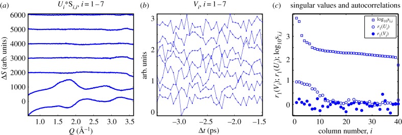
In the present case, the X matrix under consideration is the set of difference signals ΔI(Q,Δt) with n = 121 columns, each being the difference signal ΔI(Q) for m values of Q. Consequently, the ith column of U represents a typical (basis) difference scattering signal and the ith column of V represents the time evolution of this particular component. S_i,i describes the magnitude of each such component, i.e. its relative contribution to the difference signal matrix X. The left-most columns of U and V thus describe the most significant contributions to the matrix X. Decomposing ΔI(Q,Δt) in this manner, figure 2 shows the seven first columns of U (figure 2a) and V (figure 2b) and the singular values of S (figure 2c, top).

Figure 2.

Result of a singular value decomposition of the data matrix shown in figure 1. Panel (a) shows the seven first left-singular vectors U_i multiplied by their corresponding singular value, S_i,i, and offset for clarity and with U₁ lowest. Panel (b) shows the seven corresponding right-singular vectors, i.e. the seven first columns of V, where in particular the first column (lower-most trace) indicates significant time-dependence of the magnitude of U₁. Panel (c) shows, from top to bottom, the magnitude of the singular values as a function of column number i as well as the first-order autocorrelation functions of U_i and V_i. No clear cut-offs (see main text) where noise becomes a dominant part of the data are evident.

(i). Full-matrix decomposition

Following the procedure of Shrager [15] one way of addressing the noise contribution to ΔI(Q,Δt) is to construct the compressed, or rank-reduced, representation of X. This approach rests on the assumption that noise contributions are smaller than the signal and that the noise contributions are uncorrelated along m (e.g. time or concentration) and/or n (e.g. Q in scattering studies or wavelength in UV–vis spectroscopy). Under these assumptions, noise components can be identified by inspecting the set of n singular values to find a cut-off value i_cut-off after which the singular values S_i,i become very small. Alternatively, the autocorrelation function r₁(i) for the column vectors U_i and V_i can be calculated and inspected to identify the value i_cut-off where these components become noise-dominated, r₁(i) < 0.5 [15]. The compressed representation of X is then constructed by removing the columns in the U,S,V matrices with column number exceeding i_cut-off. This can massively reduce the dimensionality of the problem in, for example, least-squares fitting and improve accuracy and robustness [17].

By inspection of the right-most panel of figure 2, three singular values with large magnitudes do appear to be present, but no well-defined cut-off is immediately evident in the magnitude of S_i,i as a function of column number i. The autocorrelation of U_i gradually decays as a function of i, but with many columns where r₁(U_i) > 0.5. Only the first column vector of V has r₁(V_i) > 0.5 indicating little or no time-dependence for most of the remaining LSVs, but this result should be interpreted with caution as the spiky structure of several of the V_i vectors leads to low r₁(V_i)-values. Figure 3 illustrates the consequences of these observations when applying the rank-reduction scheme for noise suppression.

Figure 3.

Panel (a) shows the raw data, and panels (b,c) show the results of applying the effective rank method of Shrager [15]. As evident from the panel (c), retaining only one SVD component does not eliminate the significant noise/outlier contributions observed for Δt < 0 and when retaining two components, the reconstructed signal matrix contains noise at almost the same level as the raw data. (Online version in colour.)

Figure 3b,c shows the result of reducing the effective rank of the SVD decomposition to two and one, respectively. In both representations, the contribution from noise/background in the Δt < 0 part of the data matrix remains significant. This establishes rank-reduction method as unfeasible for this dataset. Based on their magnitudes relative to the signal and high auto-correlations, these contributions to the data are more properly referred to as background components or artefacts, rather than as noise. Tentatively identifying only U₂ as the main artefact contribution and setting S_2,2 before reconstructing the signal matrix significantly reduces the low-Q fluctuations, but retains the significant artefacts around Q = 1.8 Å⁻¹ (not shown).

(ii). Δt < 0 matrix decomposition

As an alternative to the rank-reduction method, we now consider another approach that relies on having obtained a good set of measurements of the background. In the present case, the subset of the ΔI(Q,Δt) matrix where constitutes such a set of measurements. As the laser pump pulses arrive significantly after the X-ray probe pulses, no structural changes owing to the laser pump pulses will contribute to this set of difference signals, only changes in detector response, air composition in the sample chamber or similar experiment-specific contributions. Figure 4 shows the result of an SVD analysis of the set of difference signals highlighted by the dashed rectangle in figure 1. The magnitude of the singular values in figure 4c indicates that two components dominate in the set of laser-off background signal, although no cut-off is evident from the autocorrelation functions of U_i and V_i.

Figure 4.

Result of a singular value decomposition of the laser-off data matrix highlighted by the black rectangle in figure 1. Panel (a) shows the seven first left-singular vectors U_i multiplied by their corresponding singular value, U_i,i. Panel (b) shows the seven corresponding right-singular vectors, i.e. the seven first columns of V. Panel (c) shows, from top to bottom, the magnitude of the singular values as a function of column number i as well as the autocorrelation functions of U_i and V_i. The magnitudes of S_i,i indicate two dominant contributions to this subset of the data, but no cut-off is evident from R(U_i) or R(V_i). (Online version in colour.)

(iii). SVD-only background fitting

The SVD analysis of the set of laser-off difference signals does not allow the algebraic reconstruction of the full dataset as employed in the rank-reduction approach above. As an alternative, a fit approach is used, in which a linear combination of N LSVs U_i determined from the background analysis are fitted to each of the 121 difference signals by minimizing the weighted residual given by

1.3

where the α_N values are free scaling parameters, σ is an estimate of the counting noise as a function of Q [12] and m is the number of Q-points in the difference signals [16]. Figure 5a shows the result of this background subtraction procedure, and from visual inspection, the background contribution is very significantly reduced when just the two most significant LSV are fitted to the data and subtracted (second panel from top). However, as evident from the lower two panels in figure 5a, including more components gradually changes the magnitude and shape of the laser-on difference signals. This observation is quantified further in figure 5b, where the average residuals for the laser-off and laser-on regions are plotted as a function of number of components used in the background subtraction procedure.

Figure 5.

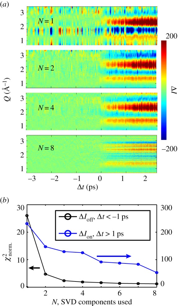
(a) From top to bottom, the four panels show the data matrix after fitting a linear combination of the first N left-singular vectors to the difference signal and then subtracting the best-fit combination. This is observed to be highly efficient in removing the noise/artefacts. (b) Average χ² (see main text for details) in the regions preceding and following t₀ as a function of number of SVD components included in the background subtraction. Three to four components are observed to efficiently eliminate the noise in the Δt < 0 region, but the background-subtracted signal for Δt > 0 is observed to also decrease as a function of the number of components included in the fit, indicating that fit approach may inadvertently remove real signal. (Online version in colour.)

These plots of residual as a function of N show that using just two background components succeeds in removing most of the background artefacts in the laser-off region. Increasing the number of components decreases the residual further. The observation of a gradually decreasing residual as a function of a number of included SVD components is not surprising, as a model with more degrees of freedom will always fit the data as well or better than some simpler model contained in the more complicated one. However, no clear cut-off in the number of SVD components to be included can be identified and the gradual change in difference signal amplitude and shape also in the Δt > 0 region of the dataset urges caution if the background-subtracted laser-on difference signals are to be used for further, detailed structural analysis.

The results presented in figure 5 indicate that one or more of the background components sufficiently resembles the actual laser-on difference signal(s) to be subtracted in the fitting-process outlined above. Such erroneous subtraction can be limited by imposing bounds on the scaling constants α₁ … α_N, where such bounds can be determined from the variation of the scaling parameter in the laser-off region. However, this only limits, but does not prevent, the subtraction of signal with possible consequences for subsequent analysis. In the following section, we present an alternative approach that relies on existing knowledge about the sample system under consideration and which uses such knowledge to limit erroneous subtraction of signal by the SVD-determined background components.

In the case of the present analysis, the sample under consideration has previously been characterized in significant detail using synchrotron sources. Through these measurements, it has been established that the Fe–N bonds rapidly (subpicosecond) expand by 0.2 Å following photo-excitation and formation of the high spin state [21,22], and tentatively that this is accompanied by a local solvent rearrangement resulting in a net density increase of the bulk solvent [10,23]. Excess energy from the photo-excitation is dissipated through vibrational relaxation leading to heating of the bulk solvent [10,24]. These structural changes lead to difference signals that for the solute can be estimated from DFT/MD simulations and, in the case of the bulk solvent, be measured in reference experiments [25,26]. These sample contributions, ΔI_sample can now be introduced in the fitting approach introduced above to yield a minization of

1.4

where

1.5

1.6

where the minimization is carried out for every time step Δt. In this expression, γ is the excitation fraction and ΔI_solute(Q) is the difference signal calculated from the known structural changes in and around the solute. ΔI_heat(Q) and ΔI_density(Q) are the hydrodynamic differentials describing the changes in scattering owing to changes in temperature (ΔT) and density (Δρ) [25,26]. γ, ΔT and Δρ are free parameters in the minimization, and the time evolution of these can provide new subpicosecond insights into both the structural dynamics taking place and on the energy dissipation following ultrafast excitation. The kinetics results obtained through this approach is beyond the scope of the present method-oriented work, but will be discussed in detail in an upcoming work [11]. Figure 6 shows the result of the background subtraction applied in the fit-based analysis presented as in figure 5 by background-subtracted difference signals. In contrast to the background-only analysis, the difference signals after background-subtraction with the model signals included are observed to be stable in the laser-on region when four or more background components are included in the subtraction procedure, both in terms of magnitude and signal shape.

Figure 6.

(a) The four panels show the data matrix after fitting a linear combination of the first N left-singular vectors and the sample-dependent difference signals to the measured data and then subtracting the best-fit SVD contribution ΔI_SVD. The inclusion of the reference signals leads to slightly less effective background subtraction, but the background-subtracted signal is now insensitive to the number N of SVD components used. (b) Summed residuals (see main text for details) in the regions preceding and following t₀ as a function of number of SVD components included in the background subtraction. The inset shows how the difference in Akaike information criterion values, ΔAICc_i, indicates N = 4−5 as optimal for background subtraction. (Online version in colour.)

From the monotonic decrease in χ² as more SVD components are included in the fits, it is difficult to identify an optimal, or correct, number of SVD components to include in the analysis. To address this issue, the (corrected) Akaike information criterion (AICc) approach to multi-model inference is introduced [27]. Briefly, the AIC measure of fit quality can be derived from information theory and provides a way of ranking a set of R competing models while taking the number of free parameters in those models into due account. A good introduction to the theory and practical applications is given by Burnham et al. [27], and following their presentation the AICc is calculated as

1.7

1.8

1.9

where P is the number of free parameters and m is the number of (independent) data points, and where χ² is normalized to this number of points, in the present case, m = 20 [12,28]. The average in the off- and on-regions (see above) were taken as input to the AIC calculation for each value of P = N + 3.

The set of R competing models can then be ranked according to their AICc-difference ΔAICc_i from the best model,

1.10

The set of models to be ranked here differ only in the number (N) of SVD components to include in the analysis. Referring to figure 6, this approach identifies the model with N = 5 as the optimal number of SVD components to include in analysis of the data presented here, but with N = 4 and N = 6 almost equally well supported by the data. A full discussion of how ΔAIC_i is formally connected to the evidence ratios between competing models and how this allows one to identify one (or more) model(s) as significantly better than other models is beyond the scope of the present work, but is given in reference [27].

The methodology outlined above represents an interpretation of experimental data within a very well-defined model framework. Given the substantial number of free parameters involved in the fit-based analysis, it is a concern whether this approach in fact imposes a certain model on the data. This could lead to the inadvertent removal of signal not explicitly included in the model. To investigate this issue, a simulation was carried out where an extra difference signal ΔI_X, taking the form of a damped sine function with maximum magnitude at Δt = 0, a lifetime of 0.5 ps and convoluted with the approximately 0.5 ps instrument response function measured for this LCLS experiment, was added to the experimental data ΔI_meas.. Such a signal shape is typical of time-resolved difference scattering signals, and the model lifetime of a few hundred femtoseconds is found for, for example, the MLCT triplet states in a series of novel Fe compounds of interest for photo-catalysis [29].

Figure 7a shows the new dataset ΔI_meas. + ΔI_X with the extra signal component shown in the inset. The magnitude of the extra signal was chosen to be fairly small compared with the real signal, as can be seen by direct comparison with figure 1. Following this addition, the new synthetic dataset was subjected to exactly the same analysis as introduced above. Figure 7b shows the residual after subtraction of all the fitted model components (ΔI_sample and ΔI_SVD) with the lower-most panel (figure 7c) showing the normalized χ² with and without inclusion of the extra signal component ΔI_X. From this representation of the analysis result, it is evident that the proposed methodology is capable of identifying signal not included in the chosen model, and that monitoring the time-dependence of the fit quality as quantified by, for example, the χ²-measure is crucial. It is, however, also evident that the signal shape of the residual is not necessarily an accurate representation of the missing signal component(s).

Figure 7.

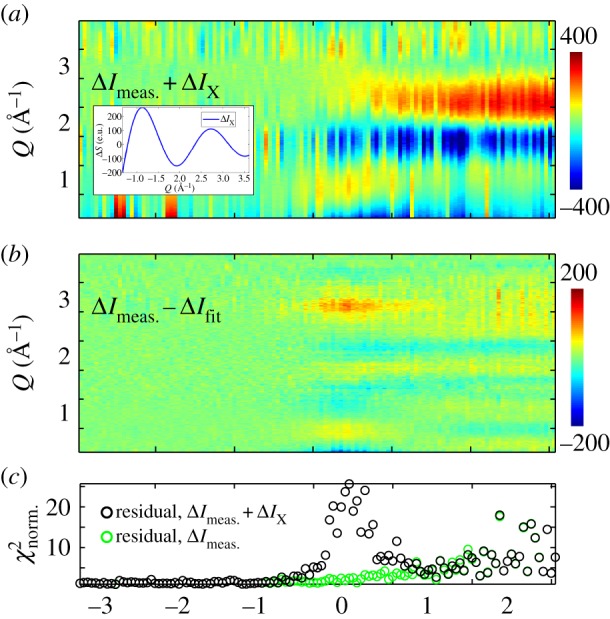
(a) Synthetic dataset with the simulated signal shown in the inset added to the original data, with a decay time of 0.5 ps. (b) Two-dimensional residual after fitting and subtracting ΔI_sample and ΔI_SVD, colour scale is half that of the panel (a). Low residual values are in general observed, but with significant residual signal present around Δt = 0 where the contribution from the added signal is strongest. (c) Normalized residual χ² as function of time delay for both the original data (green) and the synthetic data (black). The inability of the chosen model to fit the data around Δt = 0, where the extra signal has been added, is evident. (Online version in colour.)

A final aspect of the present investigation of the proposed methodology is the sensitivity of the physically interesting parameters to the magnitude of the background components and noise. To investigate this, an essentially noise-free dataset was created from the set of calculated difference signals ΔI_sample,clean(Δt) as given by equation (1.6) and with the magnitude of the (physical) scaling parameters γ, ΔT and Δρ given by the fit to the actual data for every time step Δt. The base magnitude of the SVD-determined artefacts was in a similar fashion assumed to be given by the fitting approach discussed in the preceding sections, and the level of counting noise in the original data was estimated as the standard deviation in the laser-off region of the dataset after subtraction of the SVD-determined artefacts. The simulated datasets are thus given by ΔI_sim = ΔI_sample,clean + C(ΔI_noise + ΔI_artefacts), where C is a scaling constant determining the magnitude of the noise and artefacts in the simulation.

Figure 8a shows the dependence of the mean value of each of the three physical parameters on the noise and artefact level, estimated in the Δt > 1.5 ps region (20 data points) of the dataset, where these parameters show essentially no time-dependence [11]. For, in particular, γ and Δρ an increasing trend in estimated parameter value with noise/artefact level is evident, and for all three parameters, the parameter estimates become scattered with increasing noise and artefact levels. Figure 8b shows this increase in more detail by plotting the standard variation of each parameters in the Δt > 1.5 ps region, normalized to the scatter in the analysis based on the original data. A very significant increase in the uncertainty of γ and Δρ is observed when the noise and artefact level is increased by a factor of two or more. Figure 8c shows the same plot, except in this case only the magnitude of counting noise was increased, not the magnitude of the artefacts. Ten times less sensitivity to the counting noise, compared with the sensitivity to magnitude of artefacts is observed. These results indicate that the presence of significant artefacts will adversely influence the quality of the information derived from applying the approach described in this work, even after the suggested SVD-based subtraction approach. However, for artefacts with a magnitude similar to or smaller than the signal arising from structural changes in the data, as in the present case, this effect remains limited.

Figure 8.

(a) Mean best-fit values of the three physical parameters in the model as function of noise/artefact magnitude relative to the original data. Significant drift in the parameter estimates is observed when the noise level exceeds 200% relative to the original data. (b) Variation of the parameter estimates in the steady-state (Δt > 1.5 ps) region of the data as function of noise/artefact magnitude. In particular, the excitation fraction γ shows significant variation as the noise/artefact magnitude increases and has been divided by three in this plot. (c) Variation of the parameter estimates when only the counting noise is increased. Significantly lower sensitivity to counting noise compared with artefact magnitude is observed by comparison with the panel above. (Online version in colour.)

2. Discussion and outlook

In this work, an effective method for identifying and removing significant artefact/background contributions to a given set of signals has been presented. Although it is of course always the best course to identify and correct the underlying experimental causes of such contributions, this may not always be feasible. Such is sometimes the case for time-limited experiments at facilities where access time is scarce, in particular if any deficiencies in the acquired data are subtle and only fully realized after the end of an experiment. Although fully quantifiable, the SVD-based method presented here is heuristic in nature, and further work aims to connect the proposed methodology with more rigorous schemes such as those proposed by, for example, Henry & Hofricher [30].

Regarding possible sources of the background contributions identified, a full discussion of this is beyond the scope of the present method-oriented article. However, the detector system used (CS-PAD version 1) had a spatially varying and intensity-dependent response function which is less than ideal for a highly fluctuating source such as an XFEL. Efforts were taken to limit such effects by considering only measurements in a narrow (5%) intensity interval in the analysis, but the detector response cannot be ruled out as a cause of some of the observed background fluctuations. The exact nature of this is currently being investigated in detail at both the single pixel and full-detector level and the results will be reported in future work.

The signal shape of the second-most significant LSV of the background can be qualitatively rationalized as a combination of changes air scattering (Q < 1.5 Å⁻¹) which are naturally connected with changes sample scattering intensity (Q ∼ 2 Å⁻¹) owing to any absorption changes. This can arise as a consequence of changes in the air–sample ratio along the beam path, which is not unlikely in the present experiment, as some leakage of the He bag enclosing the sample–detector set-up was observed.

The method developed and presented here relies heavily on a large body of prior work using SVD analysis for limiting noise and facilitating quantitative analysis as described in, for example, [20] and references therein. Such methods have proved highly effective in the cases where the noise and background contributions are unstructured and in general of lower magnitude than the signal itself, but the artefact-dominated character of the data discussed in this work has necessitated a development of the SVD-based methods which to the best of the author's knowledge is novel. It relies on having a good set of background measurements, as this allows robust identification and characterization of the background signal. In the present case of time-resolved measurements, this set of background measurements consisted of the set of signals for which , i.e. where the pump laser arrives at the sample position significantly after the X-ray probe pulse for all pump–probe events. Thus, the experimental conditions are as close as experimentally feasible for the laser-off and laser-on events. Rigorously, only the laser-off set of difference signals is guaranteed to be well described by a linear combination of the SVD-derived background components. However, if a given data acquisition takes only a few minutes as in the present case, then it appears reasonable to assume that the background contributions will not suddenly change character during the measurement. The fact that the assumed laser-off signals are not ‘true’ laser-off signals in the sense no laser pulse arrives at the sample may call for some caution in assuming that the laser-off signals are truly ‘dark’ signals. For this and other reasons, later experiments used the ‘drop-shot’ scheme now developed at the LCLS whereby the laser (and X-ray) shots are dropped with some selected frequency, such that, for example, every fifth laser pulse does not arrive at the sample position. Very recent investigations using this new scheme indicate that the two approaches (true dark versus negative time delay) lead to identical results, as would be expected.

The observation that a free fit followed by subtraction of background components can lead to distortion of the signal shape (figure 5) calls for some caution in how this approach is applied. However, when a good estimate of the ‘true’ signal shape is available, this can be included in the fit to limit erroneous subtraction of signal. The magnitude of the background components should be monitored for any time evolution across time-zero (Δt = 0) as this may indicate that a contribution to the difference signal from laser-induced processes in the sample may be removed by the background subtraction. Inspection of χ² is similarly crucial in order to identify situations where the model is inadequate to explain, for example, short-lived transient species. Simulations indicate some sensitivity of the physically relevant fit parameters (e.g. excitation fraction and solvent temperature increase) to the magnitudes of noise and artefacts under the proposed analysis scheme. However, these effects are limited when the background contributions have magnitudes comparable to what is observed in the acquired data. Observing such precautions, this work describes a highly effective approach to reducing spurious background contributions by an application of SVD analysis and model fits to sets of difference scattering signals with significant background noise.

References

- 1.Neutze R, Wouts R, van der Spoel D, Weckert E, Hajdu J. 2000. Potential for biomolecular imaging with femtosecond X-ray pulses. Nature 406, 752–757. ( 10.1038/35021099) [DOI] [PubMed] [Google Scholar]
- 2.Lemke HT, et al. 2013. Femtosecond X-ray absorption spectroscopy at a hard X-ray free electron laser: application to spin crossover dynamics. J. Phys. Chem. A 117, 735–740. ( 10.1021/jp312559h) [DOI] [PubMed] [Google Scholar]
- 3.Dell'Angela M, et al. 2013. Real-time observation of surface bond breaking with an X-ray laser. Science 339, 1302–1305. ( 10.1126/science.1231711) [DOI] [PubMed] [Google Scholar]
- 4.Seibert MM, et al. 2011. Single mimivirus particles intercepted and imaged with an X-ray laser. Nature 470, 78–U86. ( 10.1038/nature09748) [DOI] [PMC free article] [PubMed] [Google Scholar]
- 5.Loh ND, et al. 2012. Fractal morphology, imaging and mass spectrometry of single aerosol particles in flight. Nature 486, 513–517. ( 10.1038/nature11222) [DOI] [PubMed] [Google Scholar]
- 6.Chapman HN, et al. 2011. Femtosecond X-ray protein nanocrystallography. Nature 470, 73–U81. ( 10.1038/nature09750) [DOI] [PMC free article] [PubMed] [Google Scholar]
- 7.Vig AL, Haldrup K, Enevoldsen N, Thilsted AH, Eriksen J, Kristensen A, Feidenhans'l R, Nielsen MM. 2009. Windowless microfluidic platform based on capillary burst valves for high intensity X-ray measurements. Rev. Sci. Instrum. 80, 115114 ( 10.1063/1.3262498) [DOI] [PubMed] [Google Scholar]
- 8.Weierstall U, Spence JCH, Doak RB. 2012. Injector for scattering measurements on fully solvated biospecies. Rev. Sci. Instrum. 83, 035108 ( 10.1063/1.3693040) [DOI] [PubMed] [Google Scholar]
- 9.Hart P, et al. 2012. The CSPAD megapixel X-ray camera at LCLS. In X-ray free-electron lasers: beam diagnostics, beamline instrumentation, and applications, volume 8504 of Proceedings of SPIE. SPIE, 2012. Conf. on X-Ray Free-Electron Lasers - Beam Diagnostics, Beamline Instrumentation, and Applications (eds Moeller SP, Yabashi M, HauRiege SP.), San Diego, CA, 13–16 August 2012. [Google Scholar]
- 10.Haldrup K, et al. 2012. Guest–host interactions investigated by time-resolved X-ray spectroscopies and scattering at MHz rates: solvation dynamics and photoinduced spin transition in aqueous Fe(bipy)32+. J. Phys. Chem. A 116, 9878–9887. ( 10.1021/jp306917x) [DOI] [PubMed] [Google Scholar]
- 11.Haldrup K, et al. In preparation. [Google Scholar]
- 12.Haldrup K, Christensen M, Meedom Nielsen M. 2010. Analysis of time-resolved X-ray scattering data from solution-state systems. Acta Crystallogr. A 66, 261–269. ( 10.1107/S0108767309054233) [DOI] [PubMed] [Google Scholar]
- 13.Jun S, et al. 2010. Photochemistry of HgBr2 in methanol investigated using time-resolved X-ray liquidography. Phys. Chem. Chem. Phys. 12, 11536–11547. ( 10.1039/c002004d) [DOI] [PubMed] [Google Scholar]
- 14.Lorenz U, Møller KB, Henriksen NE. 2010. On the interpretation of time-resolved anisotropic diffraction patterns. New J. Phys. 12, 113022 ( 10.1088/1367-2630/12/11/113022) [DOI] [Google Scholar]
- 15.Shrager RI. 1986. Chemical transitions measured by spectra and resolved using singular value decomposition. Chemometr. Intell. Lab. Syst. 1, 59–70. ( 10.1016/0169-7439(86)80026-0) [DOI] [Google Scholar]
- 16.Press WH, Flannery BP, Teukolsky TA, Vetterling WT. 1986. Numerical recipes: the art of scientific computing. Cambridge, UK: Cambridge University Press. [Google Scholar]
- 17.Minh DDL, Makowski L. 2013. Wide-angle X-ray solution scattering for protein-ligand binding: multivariate curve resolution with bayesian confidence intervals. Biophys. J. 104, 873–883. ( 10.1016/j.bpj.2012.12.019) [DOI] [PMC free article] [PubMed] [Google Scholar]
- 18.Malmerberg E, et al. 2011. Time-resolved WAXS reveals accelerated conformational changes in iodoretinal-substituted proteorhodopsin. Biophys. J. 101, 1345–1353. ( 10.1016/j.bpj.2011.07.050) [DOI] [PMC free article] [PubMed] [Google Scholar]
- 19.Ren Z, Chan PWY, Moffat K, Pai EF, Royer WE, Jr, Srajer V, Yang X. 2013. Resolution of structural heterogeneity in dynamic crystallography. Acta Crystallogr. D, Biol. Crystallogr. 69, 946–959. ( 10.1107/S0907444913003454) [DOI] [PMC free article] [PubMed] [Google Scholar]
- 20.Hendler RW, Shrager RI. 1994. Deconvolutions based on singular-value decomposition and the pseudoinverse: a guide for beginners. J. Biochem. Biophys. Methods 28, 1–33. ( 10.1016/0165-022X(94)90061-2) [DOI] [PubMed] [Google Scholar]
- 21.Bressler C, et al. 2009. Femtosecond xanes study of the light-induced spin crossover dynamics in an iron(II) complex. Science 323, 489–492. ( 10.1126/science.1165733) [DOI] [PubMed] [Google Scholar]
- 22.Gawelda W, Pham VT, van der Veen RM, Grolimund D, Abela R, Chergui M, Bressler C. 2009. Structural analysis of ultrafast extended X-ray absorption fine structure with subpicometer spatial resolution: application to spin crossover complexes. J. Chem. Phys. 130, 124520 ( 10.1063/1.3081884) [DOI] [PubMed] [Google Scholar]
- 23.Daku LML, Hauser A. 2010. Ab initio molecular dynamics study of an aqueous solution of [Fe(bpy)3](Cl)2 in the low-spin and in the high-spin states. Phys. Chem. Lett. 1, 1830–1835. ( 10.1021/jz100548m) [DOI] [Google Scholar]
- 24.Consani C, Premont-Schwarz M, ElNahhas A, Bressler C, van Mourik F, Cannizzo A, Chergui M. 2009. Vibrational coherences and relaxation in the high-spin state of aqueous [FeII(bpy)3]2+. Angew. Chem. Int. Ed. 48, 7184–7187. ( 10.1002/anie.200902728) [DOI] [PubMed] [Google Scholar]
- 25.Cammarata M, et al. 2006. Impulsive solvent heating probed by picosecond X-ray diffraction. J. Chem. Phys. 124, 124504 ( 10.1063/1.2176617) [DOI] [PubMed] [Google Scholar]
- 26.Kjaer KS, et al. 2013. Introducing a standard method for experimental determination of the solvent response in laser pump, X-ray probe time-resolved wide-angle X-ray scattering experiments on systems in solution. Phys. Chem. Chem. Phys. 15, 15 003–15 016. ( 10.1039/c3cp50751c) [DOI] [PubMed] [Google Scholar]
- 27.Burnham KP, Anderson DR, Huyvaert KP. 2011. AIC model selection and multimodel inference in behavioral ecology: some background, observations, and comparisons. Behav. Ecol. Sociobiol. 65, 23–35. ( 10.1007/s00265-010-1029-6) [DOI] [Google Scholar]
- 28.Stern EA. 1993. Number of relevant independent points in x-ray absorption fine-structure spectra. Phys. Rev. B 48, 9825–9827. ( 10.1103/PhysRevB.48.9825) [DOI] [PubMed] [Google Scholar]
- 29.Liu Y, et al. 2013. Towards longer-lived metal-to-ligand charge transfer states of iron(II) complexes: an N-heterocyclic carbene approach. Chem. Commun. 49, 6412–6414. ( 10.1039/c3cc43833c) [DOI] [PubMed] [Google Scholar]
- 30.Henry E, Hofrichter J. 1992. Singular value decomposition: application to analysis of experimental-data. Methods Enzymol. 210, 129–192. [Google Scholar]