

Abstract
Fluorescence microscopy is the primary tool for studying complex processes inside individual living cells. Technical advances in both molecular biology and microscopy have made it possible to image cells from many genetic and environmental backgrounds. These images contain a vast amount of information, but this information is often hidden behind various sources of noise, convoluted with other information, and stochastic in nature. Accessing the desired biological information therefore requires new tools of computational image analysis and modeling. Here, we review some of the recent advances in computational analysis of images obtained from fluorescence microscopy, focusing on bacterial systems. We emphasize techniques that are readily available to molecular and cell biologists but also point out examples where problem-specific image analyses are necessary. Thus, image analysis is not only a toolkit to be applied to new images but is an integral part of the design and implementation of a microscopy experiment.
Keywords: bacteria, computational image analysis, fluorescence microscopy
Introduction
Light microscopy is one of the oldest techniques for studying living cells and it is used in most studies of molecular, cell, and developmental biology today [1,2]. State-of-the-art microscopes [3]and sensitive cameras paired with powerful genetically-encoded fluorescent probes [4,5]allow for high-resolution real-time observation of minimally perturbed biological processes in vivo[6–9].
Correspondingly, many studies of the location and dynamics of whole cells or of sub-cellular processes in bacteria rely on the interpretation of images obtained from brightfield and fluorescence microscopy:Imaging has been employed to gain detailed knowledge about bacterial cell shape and growth during cellular development [10–12], to study the temporal patterns of gene expression by measuring fluorescence levels or counting fluorescent molecules [13–19], to measure the motility of proteins and DNA [20–25], or to quantify protein-protein interactions[26–28 ]. The sub-cellular localization and the dynamics of protein complexes has been under scrutiny in imaging cytoskeletal proteins [29–32], the bacterial chromosome [33–37], flagellar motion [38,39], and the dynamics of molecular-motor-like proteins [40,41].
While many techniques of modern microscopy have become readily available to microbiology labs [2,42], there are few standardized tools for the analysis of the images obtained (e.g. for cell segmentation [43]; see below). Therefore, images are often analyzed by visual inspection alone, which is generally subjective and therefore entails the danger of erroneous conclusions. Visual inspection is further limited in the number of images analyzed. Therefore, computational image analysis is crucial in order to obtain consistent, statistically significant, and reliable information from imaging, and thus deserves equal attention and effort as the image acquisition itself. In fact, image analysis is often equally time-consuming or even more tedious than the processes of sample preparation and imaging themselves.
Image analysis is particularly important for the study of dynamics, where images in subsequent time frames need to be connected, as when tracking the same individual protein over multiple consecutive frames. Here, the two steps of image acquisition and analysis need to be designed together in order to extract the optimum amount of information. For example, because fluorescent proteins can only emit a limited number of photons, there is a need to fine-tune the trade-off between high signal-to-noise ratio in individual images, long duration of a time course, and a high imaging frequency.
Proper image analysis should also be accompanied by a physical or mathematical model of the biological process under study. Even if such a model is not explicitly formulated, such as during visual inspection, it is invoked consciously or subconsciously by making certain assumptions, for example about the maximum spatial displacement of proteins in subsequent time frames during tracking, or for the coincidence and proportionality of fluorescent signal and a reported gene expression level. To be certain about the proper outcome of image analysis it is thus of great importance to test the result of any analysis with respect to changes in the underlying assumptions.
In this review, we present important challenges and new developments in the computational image analysis of bacterial cells (Fig. 1), which is the field of our own studies. For specific problems for which bacterial quantitative studies are lacking, we refer to relevant works in eukaryotic cell biology, where computational image analysis has a long-standing history [44–46]. Our goal is to provide an overview of the different types of image analysis problems common today, the steps involved in each type of analysis, and the benefits of different approaches. For those interested in greater technical detail, we have referenced as many primary examples and methodology papers as possible. We regret that due to space limitations we were not able to include many excellent studies, but hope that our overview provides a good entry point for those interested in quantitative image analysis. We have also included links to available software packages that can be readily accessed.
Figure 1.
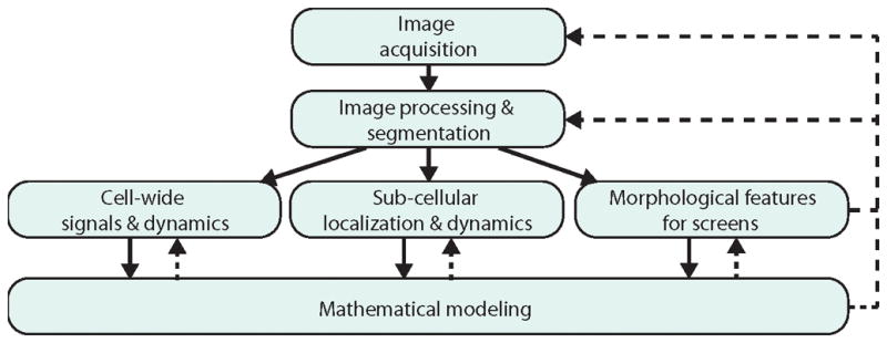
Fluorescence image analysis. Fluorescence microscopy comprises the sequential steps of image acquisition, image pre-processing, cell segmentation, and subsequent fluorescent signal analysis and interpretation. For the analysis we distinguish cases where the exact sub-cellular localization of the fluorescent signal is not required from experiments that focus on fluorescent signals that report about sub-cellular structures and loci. A third category discussed in this review focuses on signals analyzed in terms of general morphological features that can serve for microscopy screens. Generally, image interpretation requires a quantitative model of the underlying biological processes, which in turn may inform model-based image analysis techniques. To gain maximal information from fluorescence microscopy, the parameters of image acquisition, pre-processing, and analysis need to be tuned in an iterative scheme.
Image pre-processing reduces noise and enhances features
Before any information is extracted from microscopy images it is recommended and often necessary to pre-process the raw image data [47].Image pre-processing consists of correction for uneven sample illumination and photobleaching, subtraction of background signal, denoising, three-dimensional image reconstruction, and the enhancement of features such as points, lines, or edges. Most of these processes rely on filter functions that enhance or suppress certain spatial and temporal frequencies in individual images and movies. In the following, we briefly cover the processes of denoising and deconvolution, for which many tools are readily available. For more detailed information on these and other processes we refer the reader to the excellent text book by Gonzalez and Woods [47].
Noise sources include photon counting noise, camera readout noise, and background signal from auto-fluorescence. Image denoising is more important the smaller the signal-to-noise ratio, e.g. in the case of single-molecule microscopy, and if an exact quantitative knowledge of the signal is required, e.g. for studying small-number fluctuations. Denoising of 2D images is achieved by filtering with low-pass or band-pass filters that reduce single-pixel noise while retaining structural information of the objects of interest. The choice of the appropriate filter and the filter dimensions depends on the imaging process, the signal-to-noise ratio and the structures to be resolved. For time-lapse images, a three-dimensional filter might be chosen if subsequent images are significantly correlated. For images with objects of different scales, more sophisticated denoising approaches have been implemented. These methods include patch-based adaptive filtering [48] and wavelet transforms [49].The former algorithm has proven to be very efficient in low-light illumination in yeast [50].For many problems in bacteria, where the dimensions of the structures under study are comparable to the diffraction limit of light or lower, this is often not necessary and fixed-width filters are sufficient. However, the choice of the filter dimensions can be crucial for an efficient detection of the signal of interest [47]. Theoretically, determining an optimal filter design is possible, but requires a priori knowledge about the spatio-temporal auto-correlation functions of signal and noise [47]. Therefore, empirical approaches with standard filters are generally most practical and common.
The signal collected in an image pixel is not only contaminated by noise but is also convolved with signal contributions from neighboring points inside and outside the focal plane. In two-dimensional imaging, in-and out-of-plane light sources can only be distinguished if their morphology is known (e.g. if they are single fluorescent proteins). In three-dimensional imaging, a stack of images can be deconvolved using the point spread function (PSF) of the microscope objective to redistribute the blurred image intensity to the correct positions of the sources of light emission [51, 52]. The PSF of the objective can either be calculated analytically [53], measured experimentally [54,55], or estimated in a ‘blind deconvolution’ assuming certain statistical properties of the image and/or PSF [56]. Since deconvolution of the noisy image amplifies the noise and adds further artifacts to the image, denoising and deconvolution are best combined either in a single filter function or in an alternating, iterative scheme [57]. Irrespective of the particular deconvolution algorithm used, there is a tradeoff between image sharpness and noise amplification. Different deconvolution schemes are implemented in commercial software [57] and some are also available as open-source code, such as those in the ‘Clarity Deconvolution Library’ (http://cismm.cs.unc.edu/). In bacteria, three-dimensional deconvolution microscopy has been used to image the structure of a large number of proteins, including descriptions of the helix-like and ring-like structures of the bacterial cytoskeleton [58–60].
Apart from reducing noise and out-of-plane fluorescence pre-processing can also be used to enhance image features such as spots, blobs, edges, or ridges by employing corresponding filter functions [47]: For example, blobs of well-defined sizes are enhanced by a using a band-pass filter [61]. Edges and lines can be found by Canny filtering (enhancing image pixels of steep gradients), Radon and Hough transformation (identifying lines and their orientations).
Image pre-processing is thus of great importance for all sorts of image recognition tasks. For the determination of dynamic information, image pre-processing becomes even more important in order to make sure that spots, edges, or regions are robustly detected in every time frame and subsequently connected into trajectories or displacement fields (detailed in the section on tracking below).
Cell segmentation is required for establishing an intra-cellular coordinate system and for cell-morphological studies
Cell segmentation is the process of identifying and measuring the coordinates and dimensions of the borders of individual cells in an image that often contains many cells. In order to study time-dependent cell-internal processes, accurately discriminating individual cells and following them and their offspring over time is important. Furthermore, an accurate description of the cell boundaries is essential for cell-morphological studies and for determining the positions of intra-cellular events.
Cells can be segmented in different ways: The most common way is to threshold a phase-contrast image or the image of a constitutively expressed fluorescent marker. For example, in a phase-contrast image dark areas correspond to cells and light areas to background. If the cell density is low and cells don’t touch these areas correspond to cells and sub-pixel resolution can be achieved by interpolating pixel values at the boundary between high-and low-intensity pixels. For a freely available Matlab code see for example PSICIC (www.molbio1.princeton.edu/labs/gitai/psicic/psicic.html accessed on 20.12.2011) [62].If cells are in close spatial proximity the image intensity between neighboring cells might not differ enough to be recognized by initial thresholding alone. Large image areas of similar intensity then need to be separated, e.g. by iterative thresholding and filtering (see CellTracer; www.stat.duke.edu/research/software/west/celltracer/ accessed on 20.12.2011) [63]. Sub-pixel resolution can be achieved by finding edges or ridges in the image intensity as in the MicrobeTracker algorithm developed by Slisusarenko et al. (emonet.biology.yale.edu/microbetracker/accessed on 20.12.2011) [43]. This algorithm thereby combines the two qualities of identifying closely neighboring cells and determining their boundaries with sub-pixel resolution (Fig. 2). The algorithm can also be trained to learn the optimum parameters of cell segmentation. [43,62–66]
Figure 2.
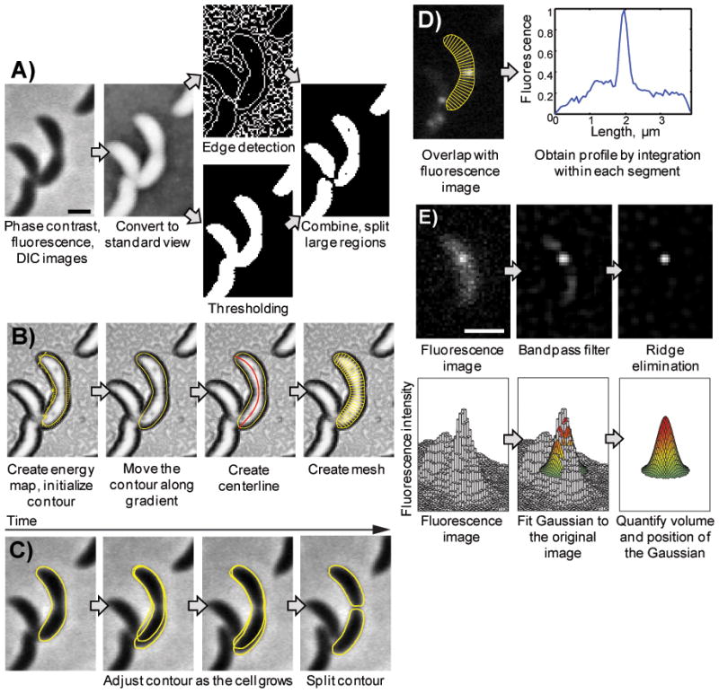
Principles of MicrobeTracker operation (Figure and caption reprinted with permission from [43]). A: Image preparation and the sequence of morphological operations with inversion, thresholding, edge and detection algorithms are shown. A phase contrast image of C. crescentus cells (MT196) expressing ftsZ-yfp is shown as an example. Bar: 1 μm. B: Active contour model and cell mesh generation. First, the energy map is generated (shown as the background), which is converted to forces (shown as arrows) and used to move a constraint active contour. The fit is considered converged when the forces drop below a certain magnitude or after a fixed number of steps. The mesh generation starts from the centerline determination and results in a creation of a set of segments of equal length along the curved cell body. C: Cell contour determination in time-lapse sequences. The active contour starts using its position from the previous frame and adjusts to the new position and shape of the cell. After that, the program checks whether the cell has divided and if so, splits the contour. D: A fluorescence profile of FtsZ-YFP signal is calculated by integration of the signal in each segment, after which the intensity can be normalized by the area or volume of the segment. E: The principles of SpotFinder operation. Top left, original fluorescence image (LacI-CFP bound to a lacO array at the chromosomal terminus;strain MT16). Top centre, the same image after processing with a bandpass filter. Top right, the same image after further processing with the ridge-removal routine. Bottom, this processed image is then used to obtain an initial guess of the position, width and height of the spots, and finally a 2D Gauss function is fit to the original image. Bar: 1 μm.
In some cases, no phase-contrast or cell-wide fluorescent signal is available but direct interference contrast (DIC) images of the cells are the only source for cell segmentation. These images have an inherent directionality that further complicates cell segmentation. For these cases Li and Canade [67]have developed a preconditioning software that transforms a DIC image into an image that can be segmented using thresholding or any of the techniques cited above. Note, however, that edges perpendicular to the wallaston prism shear axis are invisible and cannot be recovered by any type of processing.
Quantitative measurements of local concentrations help understand gene networks
Genetic circuits are inherently noisy [68,69]. In order to decipher the underlying networks and rate constants it is therefore necessary to study not only the average levels of the expressed RNA’s (such as by microarrays) and proteins (such as by Western blotting) but also their temporal fluctuations and mutual correlations in individual cells. Fluorescent proteins are great reporters for these dynamics, as their presence can be detected in single cells and with single-molecule resolution [13–15]. The challenges for analyzing such images are generally two-fold:First, determining fluorescent-protein numbers from images is difficult. Second, the number of fluorescent reporters is the result of several sequential and multiplicative stochastic processes, such that reconstructing an underlying genetic circuit from imaging data requires a model for combined transcription and translation.
There are two regimes for measuring fluorescent protein numbers: If the reporter concentration is low, individual molecules are counted by identifying and counting localized spots of fluorescent light. If the concentration is high, the fluorescent signal from each cell is integrated and translated into protein numbers. Identifying individual proteins requires that the molecules stay put during the time of image acquisition and don’t rapidly diffuse in the cell. In order to count fluorescent reporters of a large set of genes in E. coli researchers in the Xie lab therefore fused membrane proteins to the fluorescent proteins [17–19], which thus show strongly reduced diffusion during an exposure time of 100 ms. Fluorescent proteins are differentiated from the auto-fluorescence of the cell as diffraction-limited spots of 200–300 nm, if their signal is significantly higher. The latter in turn is determined by the excitation light intensity and exposure time. If the average number of fluorescent proteins per cell is much smaller than one, every light-intensity peak detected corresponds to a single fluorescent protein. If the concentration of proteins is higher, the number of fluorescent proteins represented by a single diffraction-limited spot can be determined by taking a high-frequency movie at high excitation power and making use of the discrete and stochastic bleaching of fluorescent proteins. The number of proteins is equal to the number of discrete steps of light-intensity reduction.
If the number of fluorescent proteins per cell is much higher than one, individual proteins cannot be spatially distinguished and individual bleaching events happen too frequently to be temporally resolved. Instead, the total fluorescent intensity from an individual cell is measured with much lower excitation power (in order to prevent bleaching). How is the fluorescent signal then translated into protein numbers? In pioneering work, Elowitz et al. measured the differences in fluorescence levels between symmetrically dividing daughter cells during dilution experiments and compared the probability distribution of relative differences to the expected differences of a symmetrically divided pool of protein numbers based on Poisson statistics. They thereby managed to quantify the functional relationship between fluorescent signal and protein number [64,70], that could be used as a reference for further experiments. Ultimately, their experiment allowed them to quantify the functional relationship between transcription factor concentrations and protein expression levels with the help of a biophysical model.
Once a single gene cannot be regarded in isolation, for example because it is regulated by its own transcription in a feedback loop, complex models of genetic networks or network motifs are required. Thenumber of possible models that explain the same average phenotypic behavior can be narrowed down significantly with knowledge about the temporal fluctuations of gene circuit components obtained by imaging, as shown for the transient and stochastic program of competence (uptake of foreign DNA) in Bacillus subtilis [71].
Spatial-temporal dynamics: Diffusion and motion without tracking
To quantify protein diffusion, intra-cellular transport, and cell-wide binding and unbinding events, one can exploit the otherwise undesirable property of fluorescent proteins bleaching upon illumination in a technique referred to as ‘fluorescence recovery after photobleaching’ (FRAP)[72]. Here, a focused laser beam is used to bleach the fluorescent proteins in a sub-domain of an individual cell. Afterwards, diffusion of the unbleached protein subpopulation leads to the recovery of the fluorescent signal, which can be measured as a function of time [73].
As above, the quantitative interpretation of the data obtained requires an accurate segmentation of the cell and a biophysical/biochemical model of the process underlying the recovery, because the cell boundaries alter the dynamics of the diffusing molecules. In the case of freely diffusing monomeric molecules, the fluorescence recovery can be modeled by a simple diffusion equation that takes the reflecting-boundary conditions at the cell membrane into account [20–22,24]. However, if the protein of interest is partly bound and partly free, or exists in multiple oligomeric forms, the interpretation requires a biophysical model about the diffusion, binding, and unbinding of the different potentially oligomeric forms of the molecule. In general form, such a model contains multiple binding, unbinding, and diffusion rates, as well as ratios of bound and unbound protein forms. These systems thus often require additional experimental input to close the model equations, but in certain limiting cases, such as fast diffusion of the unbound form, the analysis simplifies [73].
In addition to assisting microscopists with quantifying large numbers of images, quantitative image analysis has enabled new microscopy protocols that generate information which are not visible to the bare eye. One such technique is image-based fluorescence correlation spectroscopy (FCS). In FCS, single-pixel intensity fluctuations can be used to calculate fluorescent protein numbers and the fluorescent protein’s diffusion coefficients or reaction rate constants. For example, FCS was used to determine the absolute number of chemotaxis proteins CheY-P [74] and the local dynamics of the Min system in E.coli [23], a set of proteins that oscillates between the cell poles and thus guarantees cell division at mid-cell [75].
While FRAP and FCS can reveal information about the motility of ensembles of molecules, gaining information about the direction of motion and about the motion of individual molecules requires flow-field or tracking methods, respectively (see below).
Protein sub-cellular localization
Proteins, lipids, sugars, and DNA assemble into mesoscopic multi-subunit structures in bacteria. These large-scale structures display complex architectures and dynamics of turnover and motion that are important for their biological functions. For a detailed and molecular understanding of these processes in vivo, fluorescence imaging has proven very useful, in particular for the study of dynamics. We thus give a brief overview of high-precision localization studies in bacteria and then focus on tracking their motion in the next section. Due to the small size of bacteria, sub-cellular structures are inherently smaller or of the same length-scale as the diffraction limit of the fluorescent light (200–300nm). For determining the positions of single isolated proteins or small protein complexes, the diffraction limit does not represent a real limitation since the center of a blurry fluorescent spot can still be determined with high precision[76], for example by measuring the center of mass of the background-corrected image intensity in the area of the spot or by fitting a Gauss function to the fluorescent spot (see for example MicrobeTracker [43]). A different algorithm by Olivo-Marin[77]includes additional wavelet filtering to identify blurry spots (for a Matlab version of the code see http://lccb.hms.harvard.edu/software.html). Furthermore, many qualitatively similar custom-made algorithms have been developed for spot position determination in bacteria [78–81].
While determining the positions of single spots is only limited by the fluorescent signal, the diffraction limit does impair the accurate resolution of closely neighboring proteins. This difficulty has been overcome by reconstituting a multi-protein structure out of many images of only few stochastically or deterministically activated or excited fluorescent proteins or dyes [82,83]in techniques called PALM, FPALM, STORM, and STED. These so-called “super-resolution” imaging methods are discussed in greater technical detail in a different article in this special issue [CITATION].
In bacteria, PALM/STORM and STED hold great promise for overcoming the inherent complications of studying sub-cellular processes inside these small cells. So far, PALM/STORM has led to new insights about the sub-cellular structures of cytoskeletal proteins [84–86] and chemoreceptor receptor clusters [87]. The image analysis for all these super-resolution studies consists of single-molecule position identification by filtering, thresholding, and fitting two-dimensional Gauss curves to the blurry spots in individual frames and subsequent super-position of all peak positions into a super-resolution image [88]. As these approaches become more standardized and commercialized, we expect their use to expand significantly within the bacterial research community.
Since obtaining PALM/STORM images is relatively straightforward, the real challenge lies in extracting meaningful and biologically relevant information from these very detailed images. For example, in the work on chemoreceptor arrays in E. coli [87], Greenfield et al. extracted the distribution of array sizes. In conjunction with a mathematical model on receptor-receptor interaction they predicted that the observed receptor arrays had self-assembled without the need for any active transport.
Tracking of individual fluorescent probes and large-scale structures
Dynamical localization studies in live cells involve tracking the motion of individual molecules or the motion and morphologies of large-scale structures. To follow the directed motion of molecules or small-scale molecular complexes, fluorescent spots are either tracked individually or their collective motion is characterized by measuring a flow field. For both methods, various techniques have been developed [45]. Below, we concentrate on tracking techniques, because flow-field analysis inside bacteria is generally impractical due to their small sizes. The dynamics of large-scale structures are observed by tracking either single fluorophores attached to these structures or by following certain morphological features of the fluorescently labeled structures, such as peak or edge positions, fluorescent intensities, or overall dimensions.
A common problem in studying protein dynamics is fluorophore bleaching and blinking (i.e. switching between on and off states), stochastic processes that complicate the interpretation of single-molecule data. Bleaching introduces a tradeoff between single-frame exposure time for better localization, imaging frequency for high temporal resolution, and overall time-lapse duration. These parameters need to be tuned depending on the requirements of the subsequent image analysis [89].
In bacteria, most quantitative dynamical studies have focused on tracking fluorescent spots, representing either single or multiple closely connected fluorophores. Spot tracking requires localizing spots in individual time frames and subsequently assembling spot trajectories [89].The identification and localization of single molecules or small protein complexes is achieved as described in the previous section. If fluorescent structures are larger than the diffraction limit, they can still display a spotty fluorescent pattern, as is the case for a fluorescently labeled actin homolog MreB in E.coli [90](Fig. 3) and B.subtilis [28,41]. For example, in the work of van Teeffelen et al.[90], spots were identified with sub-pixel accuracy as the local maxima in the smoothed fluorescence image (Fig. 3).
Figure 3.
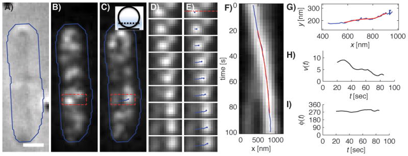
MreB persistently moves perpendicularly to the cell’s long axis in a representative cell (Figure and caption reprinted with permission from [90]). A–C: DIC (A), and smoothed fluorescence images of the initial (B) and final (C) time points of a 100 second long time lapse of two adjacent E. coli cells expressing MreB-RFPsw. The blue line indicates a rough cell outline and the scale bar is 1 μm. Inset of C) Sketch of the position of the focal plane at ~1/4 of the cell diameter (the point spread function is indicated in blue). D–E: Intermediate snapshots, taken every 12.5 seconds, of the rectangular part of the lower cell highlighted in B and C. The resulting spot trajectory is highlighted in blue in E. F: Kymograph of the interpolated fluorescence intensity along the dashed line in the first panel of E. Images were taken every 2.5 seconds. The horizontal positions of the raw (blue) and smoothed (red) trajectories are displayed. G: The raw (blue) and smoothed (red) trajectory in the xy-plane. H–I: MreB trajectory velocity v (H) and orientation relative to the long cell axis ϕ (I) as a function of time t.
If the spot density in each frame is small, spots can be connected to trajectories based on their mutual distance in subsequent frames[76], as pioneered for colloidal particles in the algorithm by Grier, Crocker, and Weeks [61] (http://www.physics.emory.edu/~weeks/idl/ accessed on 20.12.2011). Trajectories obtained in this way can then be used to extract the instantaneous speed and orientation of a spot and respective protein structure (Fig. 3G,H). However, because raw trajectories are inherently noisy, they need to be smoothed, e.g. by applying a Savitzky-Golay filter to the trajectory’s x-and y-components (Fig. 3F). The Savizky-Golay filter effectively constitutes a polynomial best fit to the trajectories, that smoothes the data but retains local extrema [91]. Note that efficient spot tracking requires careful choice of the experimental parameters (imaging frequency, exposure time, time-lapse duration) and subsequent filters (image denoising and trajectory smoothing filters) to robustly identify spots in individual frames, connect spots that represent the same proteins in subsequent frames, and also achieve a minimum overall time-lapse duration [89].Spot tracking of this kind has further been used in bacteria to track chromosome [79,86] and plasmid segregation [32], the sub-diffusive motion of chromosomal loci [25], and the linear motion of adhesion complexes in gliding Myxococcus xanthus [40]
Purely distance-based algorithms work well if the density of spots is low and if spots are robustly identified in each time frame, but there are also ways to deal with high spot densities. As in the case of resolving large-scale structures or protein distributions, the stochastic single-molecule technique PALM/STORM can be used to decrease the density to few single fluorophores and thereby allow for unambiguous single particle tracking (sptPALM) [92].For example, this approach was used quantify single-particle diffusion [93]and directed transport [94,95].
Tracking of single fluorescent proteins has the disadvantage that spots might disappear in single frames. Furthermore, even if the spot density is low, proteins can temporarily coalesce into single diffraction-limited spots. Jaqaman et al. introduced a fast algorithm that allows for spot tracking that is robust to both temporary spot disappearance and coalescence by employing a cost function based on a few user-defined parameters [96].A model-based extension of this approach is useful when the user has knowledge about the kind of motion expected (e.g. linear versus Brownian motion) or about the spot morphology (intensity, shape) [96,97].
In the case of slow dynamics, the techniques of super-resolution microscopy cited above can be extended beyond their traditional use in following single fluorophores and used to follow the movement of large-scale structures [9]. However, the imaging frequency for PALM/STORM and STED is eventually limited by the large number of independent frames required to reconstitute such a large structure with the necessary temporal resolution in the case of PALM/STORM and the inherent low frequency of scanning with STED. With PALM/STORM, a frame rate of 1/25s has been achieved for tracking the actin homolog MreB [85], which corresponds to a time scale that is comparable to the timescale of MreB’s rotational motion (Fig. 3).
In summary, the sub-cellular localization and dynamics of proteins and other macromolecules in bacteria are receiving increasing attention and quantitative studies have led to important new insights about intra-cellular processes in bacteria. Combined with more traditional genetic and biochemical approaches, modern microscopy, labeling techniques and image analysis enable mechanistic, biophysical understanding of the underlying intra-cellular processes. However, this exciting new avenue poses new challenges in quantitatively analyzing the images by computational means. Consequently, the design and implementation of quantitative image analysis methods has become just as important as the image acquisition itself.
Exploiting protein localization and dynamics for genetic screening
In the sections above we have focused on methods for carefully analyzing individual samples of interest. In addition, the power of quantitative imaging could be harnessed to enable new types of genetic or chemical screens that center on imaging-based phenotypes. In eukaryotic organisms this approach, often referred to as high content screening, has been embraced for a wide range of screens that generate huge image libraries[98–101]. This increasing amount of imaging data has made it necessary to turn to computational approaches for automating the characterization of protein location and dynamics, leading to the development of a whole new field referred to as ‘bioimage informatics’[102]. These new approaches include machine learning algorithms, which classify phenotypic differences, and model-based approaches to understand structure and dynamics. In bacteriology, the systematic and detailed study of protein localization is a much more recent domain of research [103].Accordingly, there have been only few genome-wide screens for protein location, e.g. in Escherichia coli [104]and Caulobacter crescentus [105]. As these screens become faster and increasingly automated, their image analysis will require the incorporation of automated analysis methods, as was recently demonstrated in a screen for transposon mutants in C.crescentus by Fero et al.[66]. Furthermore, synthetic biology will provide a large number of new strains that can be imaged in multiple conditions, eventually with the help of microfluidic devices [106]. Thus, more of the computational approaches that proved successful in imaging eukaryotic cells should be exploited in bacterial studies in the future [107].
Image-based screening involves image acquisition from many different samples generated under similar conditions. To screen for phenotypic differences of multiple proteins or cell components in the same experiment, fluorescent proteins of different color can be used to label these different components (see, e.g., [66]). Additional phase-contrast or DIC images give information about cell shape. The multiple images obtained from many different samples are then analyzed in the same general order as described above: first the cell outline is determined by cell segmentation, and then the fluorescent signal is quantified in one or multiple ways depending on the breadth of the scope. If the expected phenotypic differences are clearly defined in terms of image parameters (such as the position, amplitude, or speed of motion of a fluorescent spot), the analysis proceeds in the same way as described above. If, however, the anticipated phenotypic differences are not easily translated into one or few parameters extracted from the image, a learning-based algorithm with many different measures of cell morphology and fluorescent protein levels, distribution, and dynamics can be trained to classify cells according to their similarity with respect to a set of reference cells. A good example for the power of this approach comes from the screening platform CellProfiler [97]and CellProfiler Analyst [108,109](www.cellprofiler.org accessed on 20.12.2011), which were used to identify new genes involved in cell shape regulation in Drosophila cells [110]. Even if reference cells are not available, this algorithm can be used to identify new, previously non-characterized phenotypes after an iterative training session [109]. Thus, a growing number of published and publicly accessible software packages will enable automated imaging screens in bacteria in the near future.
Conclusion
Modern microbiology strongly relies on increasingly sophisticated microscopy techniques. To achieve objective and statistically significant results, the images obtained need to be analyzed computationally, which requires image preprocessing, analysis and modeling. The computational aspects of these experiments are thus often as demanding and important as the more traditional focus areas of careful sample preparation and image acquisition. Some toolkits for image analysis, including those for image pre-processing, cell segmentation, and spot localization, are readily available for any microbiologist to use. However, many imaging problems require custom image analysis that needs to be developed and adapted together with imaging acquisition and pre-processing. Furthermore, the ability to extract quantitative data can really only lead to mechanistic understanding in conjunction with careful modeling of the underlying biophysical and biochemical processes.
Abbreviations
- DIC
direct interference contrast
- FCS
fluorescence correlation spectroscopy
- FPALM
fluorescence photoactivation localization microscopy
- FRAP
fluorescence recovery after photobleaching
- PALM
photo-activated localization microscopy
- PSF
point spread function
- spt
single particle tracking
- STED
stimulated emission depletion
- STORM
stochastic optical reconstruction microscopy
Bibliography
Because of space limitations we are regrettably unable to cite all of the examples of computational image analysis in bacteria we would have liked to.
- 1.Lippincott-Schwartz J. Bridging structure and process in developmental biology through new imaging technologies. Dev Cell. 2011;21:5–10. doi: 10.1016/j.devcel.2011.06.030. [DOI] [PMC free article] [PubMed] [Google Scholar]
- 2.Dworkin J, Meyer P. Applications of fluorescence microscopy to single bacterial cells. Res Microbiol. 2007;158:187–94. doi: 10.1016/j.resmic.2006.12.008. [DOI] [PubMed] [Google Scholar]
- 3.Murphy DB. Fundamentals of light microscopy and electronic imaging. New York: Wiley-Liss; 2001. p. 368. [Google Scholar]
- 4.Piston DW, Kremers GJ, Gilbert SG, Cranfill PJ, et al. Fluorescent proteins at a glance. J Cell Sci. 2011;124:157–60. doi: 10.1242/jcs.072744. [DOI] [PMC free article] [PubMed] [Google Scholar]
- 5.Fernandez-Suarez M, Ting AY. Fluorescent probes for super-resolution imaging in living cells. Nat Rev Mol Cell Biol. 2008;9:929–43. doi: 10.1038/nrm2531. [DOI] [PubMed] [Google Scholar]
- 6.Lichtman JW, Conchello JA. Fluorescence microscopy. Nat Methods. 2005;2:910–9. doi: 10.1038/nmeth817. [DOI] [PubMed] [Google Scholar]
- 7.Xie XS, Choi PJ, Li GW, Lee NK, et al. Single-molecule approach to molecular biology in living bacterial cells. Annu Rev Biophys. 2008;37:417–44. doi: 10.1146/annurev.biophys.37.092607.174640. [DOI] [PubMed] [Google Scholar]
- 8.Leake MC, Chiu SW. Functioning nanomachines seen in real-time in living bacteria using single-molecule and super-resolution fluorescence imaging. Int J Mol Sci. 2011;12:2518–42. doi: 10.3390/ijms12042518. [DOI] [PMC free article] [PubMed] [Google Scholar]
- 9.Huang B, Babcock H, Zhuang X. Breaking the diffraction barrier: super-resolution imaging of cells. Cell. 2010;143:1047–58. doi: 10.1016/j.cell.2010.12.002. [DOI] [PMC free article] [PubMed] [Google Scholar]
- 10.Stewart EJ, Madden R, Paul G, Taddei F. Aging and death in an organism that reproduces by morphologically symmetric division. Plos Biol. 2005;3:295–300. doi: 10.1371/journal.pbio.0030045. [DOI] [PMC free article] [PubMed] [Google Scholar]
- 11.Veening JW, Stewart EJ, Berngruber TW, Taddei F, et al. Bet-hedging and epigenetic inheritance in bacterial cell development. Proc Natl Acad Sci USA. 2008;105:4393–8. doi: 10.1073/pnas.0700463105. [DOI] [PMC free article] [PubMed] [Google Scholar]
- 12.Emonet T, Sliusarenko O, Cabeen MT, Wolgemuth CW, et al. Processivity of peptidoglycan synthesis provides a built-in mechanism for the robustness of straight-rod cell morphology. ProcNatl Acad Sci USA. 2010;107:10086–91. doi: 10.1073/pnas.1000737107. [DOI] [PMC free article] [PubMed] [Google Scholar]
- 13.Elowitz MB, Locke JCW. Using movies to analyse gene circuit dynamics in single cells. Nat Rev Microbiol. 2009;7:383–92. doi: 10.1038/nrmicro2056. [DOI] [PMC free article] [PubMed] [Google Scholar]
- 14.Kentner D, Sourjik V. Use of fluorescence microscopy to study intracellular signaling in bacteria. Annu Rev Microbiol. 2010;64:373–90. doi: 10.1146/annurev.micro.112408.134205. [DOI] [PubMed] [Google Scholar]
- 15.Suel G. Use of fluorescence microscopy to analyze genetic circuit dynamics. Methods Enzymol. 2011;497:275–93. doi: 10.1016/B978-0-12-385075-1.00013-5. [DOI] [PubMed] [Google Scholar]
- 16.van Oudenaarden A, Yang Q, Pando BF, Dong GG, et al. Circadian gating of the cell cycle revealed in single cyanobacterial cells. Science. 2010;327:1522–6. doi: 10.1126/science.1181759. [DOI] [PMC free article] [PubMed] [Google Scholar]
- 17.Yu J, Xiao J, Ren X, Lao K, et al. Probing gene expression in live cells, one protein molecule at a time. Science. 2006;311:1600–3. doi: 10.1126/science.1119623. [DOI] [PubMed] [Google Scholar]
- 18.Xie XS, Li GW. Central dogma at the single-molecule level in living cells. Nature. 2011;475:308–15. doi: 10.1038/nature10315. [DOI] [PMC free article] [PubMed] [Google Scholar]
- 19.Taniguchi Y, Choi PJ, Li GW, Chen H, et al. Quantifying E. coli proteome and transcriptome with single-molecule sensitivity in single cells. Science. 2010;329:533–8. doi: 10.1126/science.1188308. [DOI] [PMC free article] [PubMed] [Google Scholar]
- 20.Elowitz MB, Surette MG, Wolf PE, Stock JB, et al. Protein mobility in the cytoplasm of Escherichia coli. J Bacteriol. 1999;181:197–203. doi: 10.1128/jb.181.1.197-203.1999. [DOI] [PMC free article] [PubMed] [Google Scholar]
- 21.Mullineaux CW, Nenninger A, Ray N, Robinson C. Diffusion of green fluorescent protein in three cell environments in Escherichia coli. J Bacteriol. 2006;188:3442–8. doi: 10.1128/JB.188.10.3442-3448.2006. [DOI] [PMC free article] [PubMed] [Google Scholar]
- 22.Sourjik V, Kumar M, Mommer MS. Mobility of cytoplasmic, membrane, and DNA-binding proteins in Escherichia coli. Biophys J. 2010;98:552–9. doi: 10.1016/j.bpj.2009.11.002. [DOI] [PMC free article] [PubMed] [Google Scholar]
- 23.Meacci G, Ries J, Fischer-Friedrich E, Kahya N, et al. Mobility of Min-proteins in Escherichia coli measured by fluorescence correlation spectroscopy. Phys Biol. 2006;3:255–63. doi: 10.1088/1478-3975/3/4/003. [DOI] [PubMed] [Google Scholar]
- 24.Weisshaar JC, Konopka MC, Shkel IA, Cayley S, et al. Crowding and confinement effects on protein diffusion in vivo. J Bacteriol. 2006;188:6115–23. doi: 10.1128/JB.01982-05. [DOI] [PMC free article] [PubMed] [Google Scholar]
- 25.Weber SC, Spakowitz AJ, Theriot JA. Bacterial chromosomal loci move subdiffusively through a viscoelastic cytoplasm. Phys Rev Lett. 2010;104:238102. doi: 10.1103/PhysRevLett.104.238102. [DOI] [PMC free article] [PubMed] [Google Scholar]
- 26.Balasubramanian MK, Srinivasan R, Mishra M, Murata-Hori M. Filament formation of the Escherichia coli actin-related protein, MreB, in fission yeast. Curr Biol. 2007;17:266–72. doi: 10.1016/j.cub.2006.11.069. [DOI] [PubMed] [Google Scholar]
- 27.Leake MC, Delalez NJ, Wadhams GH, Rosser G, et al. Signal-dependent turnover of the bacterial flagellar switch protein FliM. ProcNatl Acad Sci USA. 2010;107:11347–51. doi: 10.1073/pnas.1000284107. [DOI] [PMC free article] [PubMed] [Google Scholar]
- 28.Dominguez-Escobar J, Chastanet A, Crevenna AH, Fromion V, et al. Processive movement of MreB-associated cell wall biosynthetic complexes in bacteria. Science. 2011;333:225–8. doi: 10.1126/science.1203466. [DOI] [PubMed] [Google Scholar]
- 29.Cabeen MT, Jacobs-Wagner C. The bacterial cytoskeleton. Annu Rev Genet. 2010;44:365–92. doi: 10.1146/annurev-genet-102108-134845. [DOI] [PubMed] [Google Scholar]
- 30.Pogliano J. The bacterial cytoskeleton. Curr Opin Cell Biol. 2008;20:19–27. doi: 10.1016/j.ceb.2007.12.006. [DOI] [PubMed] [Google Scholar]
- 31.Vats P, Yu J, Rothfield L. The dynamic nature of the bacterial cytoskeleton. Cell Mol Life Sci. 2009;66:3353–62. doi: 10.1007/s00018-009-0092-5. [DOI] [PMC free article] [PubMed] [Google Scholar]
- 32.Garner EC, Campbell CS, Mullins RD. Dynamic instability in a DNA-segregating prokaryotic actin homolog. Science. 2004;306:1021–5. doi: 10.1126/science.1101313. [DOI] [PubMed] [Google Scholar]
- 33.Graumann PL. In: The Chromosome Segregation Machinery in Bacteria Bacterial Chromatin. Dame RT, Dorman CJ, editors. Springer Netherlands; 2010. pp. 31–48. [Google Scholar]
- 34.Sherratt D, Reyes-Larnothe R, Wang XD. Escherichia coli and its chromosome. Trends Microbiol. 2008;16:238–45. doi: 10.1016/j.tim.2008.02.003. [DOI] [PubMed] [Google Scholar]
- 35.Rocha EPC. The organization of the bacterial genome. Annu RevGenet. 2008;42:211–33. doi: 10.1146/annurev.genet.42.110807.091653. [DOI] [PubMed] [Google Scholar]
- 36.Thanbichler M, Shapiro L. Getting organized – how bacterial cells move proteins and DNA. Nat Rev Microbiol. 2008;6:28–40. doi: 10.1038/nrmicro1795. [DOI] [PubMed] [Google Scholar]
- 37.Gerdes K, Howard M, Szardenings F. Pushing and pulling in prokaryotic DNA segregation. Cell. 2010;141:927–42. doi: 10.1016/j.cell.2010.05.033. [DOI] [PubMed] [Google Scholar]
- 38.Berg HC. E. coli in motion. New York: Springer; 2004. p. 133. [Google Scholar]
- 39.Copeland MF, Flickinger ST, Tuson HH, Weibel DB. Studying the dynamics of flagella in multicellular communities of Escherichia coli by using biarsenical dyes. Appl Environ Microbiol. 2010;76:1241–50. doi: 10.1128/AEM.02153-09. [DOI] [PMC free article] [PubMed] [Google Scholar]
- 40.Shaevitz JW, Sun MZ, Wartel M, Cascales E, et al. Motor-driven intracellular transport powers bacterial gliding motility. ProcNatl Acad Sci USA. 2011;108:7559–64. doi: 10.1073/pnas.1101101108. [DOI] [PMC free article] [PubMed] [Google Scholar]
- 41.Garner EC, Bernard R, Wang WQ, Zhuang XW, et al. Coupled, circumferential motions of the cell wall synthesis machinery and MreB filaments in B. subtilis. Science. 2011;333:222–5. doi: 10.1126/science.1203285. [DOI] [PMC free article] [PubMed] [Google Scholar]
- 42.Gitai Z. New fluorescence microscopy methods for microbiology: sharper, faster, and quantitative. Curr Opin Microbiol. 2009;12:341–6. doi: 10.1016/j.mib.2009.03.001. [DOI] [PMC free article] [PubMed] [Google Scholar]
- 43.Emonet T, Sliusarenko O, Heinritz J, Jacobs-Wagner C. High-throughput, subpixel precision analysis of bacterial morphogenesis and intracellular spatio-temporal dynamics. Mol Microbiol. 2011;80:612–27. doi: 10.1111/j.1365-2958.2011.07579.x. [DOI] [PMC free article] [PubMed] [Google Scholar]
- 44.Meijering E, Dzyubachyk O, Smal I, van Cappellen WA. Tracking in cell and developmental biology. Semin Cell Dev Biol. 2009;20:894–902. doi: 10.1016/j.semcdb.2009.07.004. [DOI] [PubMed] [Google Scholar]
- 45.Dorn JF, Danuser G, Yang G. Computational processing and analysis of dynamic fluorescence image data. Methods Cell Biol. 2008;85:497–538. doi: 10.1016/S0091-679X(08)85022-4. [DOI] [PubMed] [Google Scholar]
- 46.Goldman RD, Swedlow J, Spector DL. Live cell imaging : a laboratory manual. xvi. Cold Spring Harbor, N.Y: Cold Spring Harbor Laboratory Press; 2010. p. 736. [Google Scholar]
- 47.Gonzalez RC, Woods RE. Digital image processing. xxii. Upper Saddle River, N.J: Prentice Hall; 2008. p. 954. [Google Scholar]
- 48.Boulanger J, Kervrann C, Bouthemy P, Elbau P, et al. Patch-based nonlocal functional for denoising fluorescence microscopy image sequences. IEEE TMed Imaging. 2010;29:442–54. doi: 10.1109/TMI.2009.2033991. [DOI] [PubMed] [Google Scholar]
- 49.Luisier F, Vonesch C, Blu T, Unser M. Fast Haar-wavelet denoising of multidimensional fluorescence microscopy data. Biomedical Imaging: From Nano to Macro, 2009. ISBI ‘09. IEEE International Symposium on; 2009. pp. 310–3. [Google Scholar]
- 50.Sedat JW, Carlton PM, Boulanger J, Kervrann C, et al. Fast live simultaneous multiwavelength four-dimensional optical microscopy. Proc Natl Acad Sci USA. 2010;107:16016–22. doi: 10.1073/pnas.1004037107. [DOI] [PMC free article] [PubMed] [Google Scholar]
- 51.Agard DA, Hiraoka Y, Shaw P, Sedat JW. Chapter 13 Fluorescence Microscopy in Three Dimensions. In: Taylor DL, Yu-Li W, editors. Methods in Cell Biology. Academic Press; 1989. pp. 353–77. [DOI] [PubMed] [Google Scholar]
- 52.Wallace W, Schaefer LH, Swedlow JR. A workingperson’s guide to deconvolution in light microscopy. Biotechniques. 2001;31:1076–97. doi: 10.2144/01315bi01. [DOI] [PubMed] [Google Scholar]
- 53.Gibson SF, Lanni F. Experimental test of an analytical model of aberration in an oil-immersion objective lens used in 3-dimensional light-microscopy. J Opt Soc Am A. 1991;8:1601–13. doi: 10.1364/josaa.9.000154. [DOI] [PubMed] [Google Scholar]
- 54.De Mey JR, Kessler P, Dompierre J, Cordelieres FP, et al. Fast 4D microscopy. Method Cell Biol. 2008;85:83–112. doi: 10.1016/S0091-679X(08)85005-4. [DOI] [PubMed] [Google Scholar]
- 55.Shaevitz JW, Fletcher DA. Enhanced three-dimensional deconvolution microscopy using a measured depth-varying point-spread function. J Opt Soc Am A. 2007;24:2622–7. doi: 10.1364/josaa.24.002622. [DOI] [PubMed] [Google Scholar]
- 56.Holmes TJ. Blind deconvolution of quantum-limited incoherent imagery -maximum-likelihood approach. J Opt Soc Am A. 1992;9:1052–61. doi: 10.1364/josaa.9.001052. [DOI] [PubMed] [Google Scholar]
- 57.McNally JG, Karpova T, Cooper J, Conchello JA. Three-dimensional imaging by deconvolution microscopy. Methods. 1999;19:373–85. doi: 10.1006/meth.1999.0873. [DOI] [PubMed] [Google Scholar]
- 58.Gober JW, Figge RM, Divakaruni AV. MreB, the cell shape-determining bacterial actin homologue, co-ordinates cell wall morphogenesis in Caulobacter crescentus. Mol Microbiol. 2004;51:1321–32. doi: 10.1111/j.1365-2958.2003.03936.x. [DOI] [PubMed] [Google Scholar]
- 59.Gitai Z, Dye N, Shapiro L. An actin-like gene can determine cell polarity in bacteria. ProcNatl Acad Sci USA. 2004;101:8643–8. doi: 10.1073/pnas.0402638101. [DOI] [PMC free article] [PubMed] [Google Scholar]
- 60.Armitage JP, Slovak PM, Wadhams GH. Localization of MreB in Rhodobacter sphaeroides under conditions causing changes in cell shape and membrane structure. J Bacteriol. 2005;187:54–64. doi: 10.1128/JB.187.1.54-64.2005. [DOI] [PMC free article] [PubMed] [Google Scholar]
- 61.Crocker JC, Grier DG. Methods of digital video microscopy for colloidal studies. J Colloid Interf Sci. 1996;179:298–310. [Google Scholar]
- 62.Guberman JM, Fay A, Dworkin J, Wingreen NS, et al. PSICIC: Noise and asymmetry in bacterial division revealed by computational image analysis at sub-pixel resolution. PLoS Comput Biol. 2008;4:e1000233. doi: 10.1371/journal.pcbi.1000233. [DOI] [PMC free article] [PubMed] [Google Scholar]
- 63.Wang Q, Niemi J, Tan CM, You L, et al. Image segmentation and dynamic lineage analysis in single-cell fluorescence microscopy. Cytometry A. 2010;77:101–10. doi: 10.1002/cyto.a.20812. [DOI] [PMC free article] [PubMed] [Google Scholar]
- 64.Elowitz MB, Rosenfeld N, Young JW, Alon U, et al. Gene regulation at the single-cell level. Science. 2005;307:1962–5. doi: 10.1126/science.1106914. [DOI] [PubMed] [Google Scholar]
- 65.Itan E, Carmon G, Rabinovitch A, Fishov I, et al. Shape of nonseptated Escherichia coli is asymmetric. Phys Rev E Stat Nonlin Soft Mater Phys. 2008;77:061902. doi: 10.1103/PhysRevE.77.061902. [DOI] [PubMed] [Google Scholar]
- 66.Fero MJ, Christen B, Hillson NJ, Bowman G, et al. High-throughput identification of protein localization dependency networks. ProcNatl Acad Sci USA. 2010;107:4681–6. doi: 10.1073/pnas.1000846107. [DOI] [PMC free article] [PubMed] [Google Scholar]
- 67.Li K, Kanade T. Nonnegative Mixed-Norm Preconditioning for Microscopy Image Segmentation. In: Prince J, Pham D, Myers K, editors. Information Processing in Medical Imaging. Springer; Berlin/Heidelberg: 2009. pp. 362–73. [DOI] [PubMed] [Google Scholar]
- 68.Losick R, Desplan C. Stochasticity and cell fate. Science. 2008;320:65–8. doi: 10.1126/science.1147888. [DOI] [PMC free article] [PubMed] [Google Scholar]
- 69.Eldar A, Elowitz MB. Functional roles for noise in genetic circuits. Nature. 2010;467:167–73. doi: 10.1038/nature09326. [DOI] [PMC free article] [PubMed] [Google Scholar]
- 70.Rosenfeld N, Perkins TJ, Alon U, Elowitz MB, et al. A fluctuation method to quantify in vivo fluorescence data. Biophys J. 2006;91:759–66. doi: 10.1529/biophysj.105.073098. [DOI] [PMC free article] [PubMed] [Google Scholar]
- 71.Cagatay T, Turcotte M, Elowitz MB, Garcia-Ojalvo J, et al. Architecture-dependent noise discriminates functionally analogous differentiation circuits. Cell. 2009;139:512–22. doi: 10.1016/j.cell.2009.07.046. [DOI] [PubMed] [Google Scholar]
- 72.Lippincott-Schwartz J, Altan-Bonnet N, Patterson GH. Photobleaching and photoactivation: following protein dynamics in living cells. Nat Cell Biol. 2003;(Suppl):S7–14. [PubMed] [Google Scholar]
- 73.McNally JG. Quantitative FRAP in analysis of molecular binding dynamics in vivo. Methods Cell Biol. 2008;85:329–51. doi: 10.1016/S0091-679X(08)85014-5. [DOI] [PubMed] [Google Scholar]
- 74.Cluzel P, Surette M, Leibler S. An ultrasensitive bacterial motor revealed by monitoring signaling proteins in single cells. Science. 2000;287:1652–5. doi: 10.1126/science.287.5458.1652. [DOI] [PubMed] [Google Scholar]
- 75.Lutkenhaus J. Assembly dynamics of the bacterial MinCDE system and spatial regulation of the Z ring. Annu Rev Biochem. 2007;76:539–62. doi: 10.1146/annurev.biochem.75.103004.142652. [DOI] [PubMed] [Google Scholar]
- 76.Cheezum MK, Walker WF, Guilford WH. Quantitative comparison of algorithms for tracking single fluorescent particles. Biophys J. 2001;81:2378–88. doi: 10.1016/S0006-3495(01)75884-5. [DOI] [PMC free article] [PubMed] [Google Scholar]
- 77.Olivo-Marin JC. Extraction of spots in biological images using multiscale products. Pattern Recogn. 2002;35:1989–96. [Google Scholar]
- 78.Viollier PH, Thanbichler M, McGrath PT, West L, et al. Rapid and sequential movement of individual chromosomal loci to specific subcellular locations during bacterial DNA replication. Proc Natl Acad Sci USA. 2004;101:9257–62. doi: 10.1073/pnas.0402606101. [DOI] [PMC free article] [PubMed] [Google Scholar]
- 79.Gitai Z, Shebelut CW, Guberman JM, van Teeffelen S, et al. Caulobacter chromosome segregation is an ordered multistep process. Proc Natl Acad Sci USA. 2010;107:14194–8. doi: 10.1073/pnas.1005274107. [DOI] [PMC free article] [PubMed] [Google Scholar]
- 80.Keiler KC, Russell JH. Subcellular localization of a bacterial regulatory RNA. ProcNatl Acad Sci USA. 2009;106:16405–9. doi: 10.1073/pnas.0904904106. [DOI] [PMC free article] [PubMed] [Google Scholar]
- 81.Montero Llopis P, Jackson AF, Sliusarenko O, Surovtsev I, et al. Spatial organization of the flow of genetic information in bacteria. Nature. 2010;466:77–81. doi: 10.1038/nature09152. [DOI] [PMC free article] [PubMed] [Google Scholar]
- 82.Schermelleh L, Heintzmann R, Leonhardt H. A guide to super-resolution fluorescence microscopy. J Cell Biol. 2010;190:165–75. doi: 10.1083/jcb.201002018. [DOI] [PMC free article] [PubMed] [Google Scholar]
- 83.Thompson MA, Biteen JS, Lord SJ, Conley NR, et al. Molecules and methods for super-resolution imaging. Methods Enzymol. 2010;475:27–59. doi: 10.1016/S0076-6879(10)75002-3. [DOI] [PMC free article] [PubMed] [Google Scholar]
- 84.Guo F, Tao HA, Buss J, Coltharp C, et al. In vivo structure of the E. coli FtsZ-ring revealed by photoactivated localization microscopy (PALM) Plos One. 2010;5:e12682. doi: 10.1371/journal.pone.0012680. [DOI] [PMC free article] [PubMed] [Google Scholar]
- 85.Biteen JS, Thompson MA, Tselentis NK, Bowman GR, et al. Super-resolution imaging in live Caulobacter crescentus cells using photoswitchable EYFP. Nat Methods. 2008;5:947–9. doi: 10.1038/NMETH.1258. [DOI] [PMC free article] [PubMed] [Google Scholar]
- 86.Ptacin JL, Lee SF, Garner EC, Toro E, et al. A spindle-like apparatus guides bacterial chromosome segregation. Nat Cell Biol. 2010;12:791–8. doi: 10.1038/ncb2083. [DOI] [PMC free article] [PubMed] [Google Scholar]
- 87.Greenfield D, McEvoy AL, Shroff H, Crooks GE, et al. Self-organization of the Escherichia coli chemotaxis network imaged with super-resolution light microscopy. Plos Biol. 2009;7:e1000137. doi: 10.1371/journal.pbio.1000137. [DOI] [PMC free article] [PubMed] [Google Scholar]
- 88.Betzig E, Patterson GH, Sougrat R, Lindwasser OW, et al. Imaging intracellular fluorescent proteins at nanometer resolution. Science. 2006;313:1642–5. doi: 10.1126/science.1127344. [DOI] [PubMed] [Google Scholar]
- 89.Jaqaman K, Danuser G. Computational image analysis of cellular dynamics: a case study based on particle tracking. Cold Spring Harb Protoc. 2009;2009 doi: 10.1101/pdb.top65. pdb top65. [DOI] [PMC free article] [PubMed] [Google Scholar]
- 90.van Teeffelen S, Wang S, Furchtgott L, Huang KC, et al. The bacterial actin MreB rotates, and rotation depends on cell-wall assembly. Proc Natl Acad Sci USA. 2011;108:15822–7. doi: 10.1073/pnas.1108999108. [DOI] [PMC free article] [PubMed] [Google Scholar]
- 91.Savitzky A, Golay MJE. Smoothing and differentiation of data by simplified least squares procedures. Anal Chem. 1964;36:1627–39. [Google Scholar]
- 92.Manley S, Gillette JM, Patterson GH, Shroff H, et al. High-density mapping of single-molecule trajectories with photoactivated localization microscopy. Nat Methods. 2008;5:155–7. doi: 10.1038/nmeth.1176. [DOI] [PubMed] [Google Scholar]
- 93.Niu L, Yu J. Investigating intracellular dynamics of FtsZ cytoskeleton with photoactivation single-molecule tracking. Biophys J. 2008;95:2009–16. doi: 10.1529/biophysj.108.128751. [DOI] [PMC free article] [PubMed] [Google Scholar]
- 94.Kim SY, Gitai Z, Kinkhabwala A, Shapiro L, et al. Single molecules of the bacterial actin MreB undergo directed treadmilling motion in Caulobacter crescentus. Proc Natl Acad Sci USA. 2006;103:10929–34. doi: 10.1073/pnas.0604503103. [DOI] [PMC free article] [PubMed] [Google Scholar]
- 95.Bowman GR, Comolli LR, Zhu J, Eckart M, et al. A polymeric protein anchors the chromosomal origin/ParB complex at a bacterial cell pole. Cell. 2008;134:945–55. doi: 10.1016/j.cell.2008.07.015. [DOI] [PMC free article] [PubMed] [Google Scholar]
- 96.Jaqaman K, Loerke D, Mettlen M, Kuwata H, et al. Robust single-particle tracking in live-cell time-lapse sequences. Nat Methods. 2008;5:695–702. doi: 10.1038/nmeth.1237. [DOI] [PMC free article] [PubMed] [Google Scholar]
- 97.Sabatini DM, Carpenter AE, Jones TR, Lamprecht MR, et al. CellProfiler: image analysis software for identifying and quantifying cell phenotypes. Genome Biol. 2006;7:R100. doi: 10.1186/gb-2006-7-10-r100. [DOI] [PMC free article] [PubMed] [Google Scholar]
- 98.Murphy RF. An active role for machine learning in drug development. Nat Chem Biol. 2011;7:327–30. doi: 10.1038/nchembio.576. [DOI] [PMC free article] [PubMed] [Google Scholar]
- 99.Carpenter AE. Image-based chemical screening. Nat Chem Biol. 2007;3:461–5. doi: 10.1038/nchembio.2007.15. [DOI] [PubMed] [Google Scholar]
- 100.Eggert US, Mitchison TJ. Small molecule screening by imaging. Curr Opin Chem Biol. 2006;10:232–7. doi: 10.1016/j.cbpa.2006.04.010. [DOI] [PubMed] [Google Scholar]
- 101.Goshima G, Wollman R, Goodwin SS, Zhang N, et al. Genes required for mitotic spindle assembly in Drosophila S2 cells. Science. 2007;316:417–21. doi: 10.1126/science.1141314. [DOI] [PMC free article] [PubMed] [Google Scholar]
- 102.Peng HC. Bioimage informatics: a new area of engineering biology. Bioinformatics. 2008;24:1827–36. doi: 10.1093/bioinformatics/btn346. [DOI] [PMC free article] [PubMed] [Google Scholar]
- 103.Shapiro L, McAdams HH, Losick R. Why and how bacteria localize proteins. Science. 2009;326:1225–8. doi: 10.1126/science.1175685. [DOI] [PMC free article] [PubMed] [Google Scholar]
- 104.Mori H, Kitagawa M, Ara T, Arifuzzaman M, et al. Complete set of ORF clones of Escherichia coli ASKA library (A complete Set of E. coli K-12 ORF archive): Unique resources for biological research. DNA Res. 2005;12:291–9. doi: 10.1093/dnares/dsi012. [DOI] [PubMed] [Google Scholar]
- 105.Gitai Z, Werner JN, Chen EY, Guberman JM, et al. Quantitative genome-scale analysis of protein localization in an asymmetric bacterium. ProcNatl Acad Sci USA. 2009;106:7858–63. doi: 10.1073/pnas.0901781106. [DOI] [PMC free article] [PubMed] [Google Scholar]
- 106.Szita N, Polizzi K, Jaccard N, Baganz F. Microfluidic approaches for systems and synthetic biology. Curr Opin Biotech. 2010;21:517–23. doi: 10.1016/j.copbio.2010.08.002. [DOI] [PubMed] [Google Scholar]
- 107.Fero M, Pogliano K. Automated quantitative live cell fluorescence microscopy. Cold Spring HarbPerspect Biol. 2010;2:a000455. doi: 10.1101/cshperspect.a000455. [DOI] [PMC free article] [PubMed] [Google Scholar]
- 108.Jones TR, Kang IH, Wheeler DB, Lindquist RA, et al. CellProfiler Analyst: data exploration and analysis software for complex image-based screens. Bmc Bioinformatics. 2008;9:482. doi: 10.1186/1471-2105-9-482. [DOI] [PMC free article] [PubMed] [Google Scholar]
- 109.Jones TR, Carpenter AE, Lamprecht MR, Moffat J, et al. Scoring diverse cellular morphologies in image-based screens with iterative feedback and machine learning. Proc Natl Acad Sci USA. 2009;106:1826–31. doi: 10.1073/pnas.0808843106. [DOI] [PMC free article] [PubMed] [Google Scholar]
- 110.Bakal C, Aach J, Church G, Perrimon N. Quantitative morphological signatures define local signaling networks regulating cell morphology. Science. 2007;316:1753–6. doi: 10.1126/science.1140324. [DOI] [PubMed] [Google Scholar]