

Abstract
This contribution describes the use of small and wide angle X-ray and small angle neutron scattering for biomolecular structure calculation using the program Xplor-NIH, both with and without NMR data. The current algorithms used for calculating scattering curves are described, and the use of scattering data as a structural restraint is given concrete form as a fragment of an Xplor-NIH structure calculation script. We review five examples of the use of scattering data in structure calculation, including the treatment of single domain proteins, nucleic acids, structure determination of large proteins, and the use of ensemble representations to characterize small and large amplitude motions.
Keywords: Structure Determination, SAXS, WAXS, SANS, NMR Restraints, Proteins, Nucleic Acids
1. Introduction
The most commonly used NMR-derived restraints consist of approximate, short range (< 6 Å) inter-proton distances and backbone torsion angles, both of which are local in nature [1]. It is also common to include residual dipolar coupling (RDC) data which provide orientational information for bond vectors relative to an external alignment tensor [2]. Small and wide angle X-ray scattering (SAXS/WAXS) and small angle neutron scattering (SANS) data, on the other hand, provide information on overall molecular size, shape and dominant intermolecular distances [3, 4]. Thus, solution NMR and scattering data provide highly complementary structural information.
SAXS data was first systematically used in joint NMR structure calculations by Grishaev et. al. [5], where the use of SAXS data was shown to improve the structure of the γS crystallin homodimer relative to that determined with NMR data alone. These initial calculations involved direct computation of the Debye formula [6], which scales as the square of N, the number of atoms, and as such, is limited to relatively small systems. Shortly thereafter, an approximate algorithm which scales linearly with N was implemented in Xplor-NIH [7], and has since been used for structure calculation of large systems, as is demonstrated below. An alternative approximate approach [8] employs only the small-angle portion of a SAXS or SANS curve, thus losing much information content.
In this review, we describe the facilities for joint NMR - small-angle solution scattering (SASS) within the Xplor-NIH molecular structure determination package [9, 10]. We then present five examples of the use of these facilities in structure determination. Finally, we review the prospects for future development of NMR/SASS methods for molecular structure determination.
2. Solution X-Ray scattering calculation
Given a plane wave of X-ray radiation incident on a molecule in solution, the scattering amplitude is approximated as
| (1) |
where q is reciprocal space scattering vector with amplitude q, j sums over all atoms, is the effective atomic scattering form factor, xj is the position of atom j, k sums over points representing boundary-associated solvent, and and yk are, respectively, the positions and scattering form factors of these points. In Eq. (1), the first sum arises from scattering by each solute atom relative to that expected for an equivalent volume of displaced solvent, while the second sum which arises from scattering by solvent bound to the molecular surface, is less important and will be treated below. q is related to the experimental scattering angle 2θ by
| (2) |
where λ is the wavelength of the incident radiation. θ = 0 corresponds to the forward scattering direction.
The effective atomic scattering amplitude can be written
| (3) |
where fj(q) is the vacuum atomic scattering amplitude, ρs is the bulk solvent electron density, and gj is a scattering factor due to excluded solvent [11, 12], which is taken to be
| (4) |
where Vj is the volume of atom j, rm is the radius corresponding to the average atomic volume, and sV and sr are scale factors which take values close to one, and whose values are typically determined using a fit to experimental data, as in Ref. [12]. The values of are precomputed using standard expressions [5, 13] for atomic scattering amplitudes and the solvent scattering factors.
In solution, averaging is performed over reciprocal space solid angle such that the observed intensity is
| (5) |
where ⟨·⟩Ω denotes average over solid angle. Omitting the boundary scattering contribution, this average can be expressed in closed form to yield the Debye formula:
| (6) |
where the sum is over all pairs of atoms, rij is the inter-atomic distance, and sinc(x) = sin(x)/x.
For refinement purposes, Eq. (6) is generally too expensive for use in its raw form, as it scales as the square of the number of atoms. We employ two approximations to make the computation of I(q) tractable for refinement, including approximating Eq. (5) by averaging ∣A(q)∣2 computed at discrete points on the surface of a sphere, and through judicious use of atom-globing [14, 15].
From Eq. (1) we see that the scattering amplitude due to a group of atoms is linear in the number of atoms, so it makes sense to compute amplitude instead of intensity. We can then obtain the scattering intensity by numerically integrating Eq. (5). We find that if the points are taken uniformly on the surface of the sphere (e.g. the spiral algorithm [16]), relatively few points are required to obtain a good approximation to Eq. (6). For biomolecular systems, we found that I(q) is well-represented by tens of points at small scattering amplitudes, and up to hundreds of points at the larger values of q sampled in our studies. When the number of grid points is not quite large enough, the current method seems to fail gracefully (the resulting error grows slowly with increasing q).
Additional speedup is possible with this approach if we sample I(q) at equally spaced values of q and if the surface grid on which A(q) is evaluated is reused at each value of q. In this case, atom j’s contribution to A(q) is
| (7) |
where q = qmin + nΔq, Δq is the spacing in q, and is a unit vector in the direction of q. Thus, the exponential term exp is computed once for each atom (for n = 1) at each reciprocal space angular grid point corresponding to , and the values of the contribution at other values of q are obtained by simple multiplication.
In addition to the finite difference approximation to the integral in Eq. (5), we employ the globbing approximation used by others [5, 14, 15, 17]. In this approximation, the contribution of multiple atoms is approximated by a scattering center at the average atom position (weighted by number of electrons) with the following scattering amplitude:
| (8) |
where the sum is over all atoms in the glob. We typically use globs consisting of at most three atoms. As in [5], we use a multiplicative q-dependent correction factor c(q) to correct for the errors introduced by globbing:
| (9) |
where Iapprox(q) is the scattering intensity obtained using the globic scattering factors. To speed calculation of the scattering curve during molecular dynamics we typically evaluate Iapprox using a relatively coarse solid angle grid in the numerical evaluation of Eq. (5) and also omit the explicit dependence of the boundary solvent scattering. The resulting approximate curve is periodically corrected by computing a more accurate, but computationally expensive scattering intensity Ifine(q) with no globs, using a finer grid of reciprocal space angles, and including the effects of bound-solvent scattering. The correction factor is then computed as
| (10) |
which is used until the next computation of Ifine(q). To give an idea of the calculation times for the 128 kDa Enzyme I homodimer (PDB entry 2XDF) [18], a routine calculation on a contemporary computer core of I(q) over 100 points using an angular grid with 50 points in reciprocal space and atom globbing takes about 0.05 s, while a correction calculation using no globbing and an angular grid of 500 points takes about 1.9 s. For comparison, the calculation using the exact Debye expression takes about 110 s for this molecule.
2.1. Boundary Layer Contribution
In Eq. (1) each boundary scatterer at position yk has an effective form factor
| (11) |
corresponding to a sphere of radius rk with uniform density ρb. The positions and radii of the boundary points are computed as described below.
We use the method of Varshney, et. al [19] to compute a molecular surface description defined as a triangular mesh and computed outward-pointing surface normals. In our approximate description of the boundary region, we use the Varshney algorithm to generate the outer surface described by rolling a solvent molecule of radius rw over atoms of radius ri + rb, where ri is the atomic radius as specified in Ref. [12] and rb is the boundary layer thickness. The inner surface of the boundary region is generated from the outer triangular mesh surface, by extending, for each vertex, a line segment of length rb in the direction opposite the surface normal. We generally use rw = 1.44 Å and rb = 3 Å.
Each triangle on the outer surface and its compliment on the inner surface bound an irregular triangular prism as depicted in Figure 1. In our boundary layer description the contribution of each prism is represented as a sphere of uniform density such that each region contributes to the second sum in Eq. (1): yk is taken to be the center of the prism, and rk the radius corresponding to a sphere whose volume is that of the prism.
Figure 1.
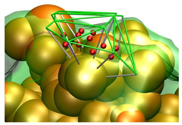
Visualization of a portion of the boundary layer scatterers. The green lines depict a portion of the tessellated surface generated using atomic radii (+ 3 Å). An inner surface (transparent green surface) was generated by dropping line segments (white lines) 3Å in the direction opposite the surface normals at each vertex. A scattering center (red) was located at the center of each voxel at yk defined by outer and inner triangular patches. The orange spheres correspond to heavy atoms of the molecule. The scattering from each voxel is represented as a sphere of uniform density and radius rk, corresponding to the voxel’s volume. Adapted from Schwieters et. al. [18] published in J. Am. Chem. Soc. (American Chemical Society) while the authors were U.S. Government employees at the National Institutes of Health.
While approximate, such a surface description has the advantage of describing surfaces with complex shape, including concave regions, while the surface description of Svergun et. al. [12] fails to capture bound solvent contribution in such cases.
As in Ref [12], the three parameters sV, sr, and ρb describing the solvent scattering contribution are fit using a grid search. These parameters are recomputed periodically throughout the structure determination, and the effect on calculated scattering intensity included in the correction factor c(q). As the boundary layer contribution to the scattering intensity is not recalculated during every dynamics time step, a discontinuity in the energy occurs when c(q) is recomputed. This is accommodated by recomputing c(q) at the beginning of molecular dynamics runs at each temperature during simulated annealing, and again after final minimization.
2.1.1. SANS Calculation
The procedure for calculation of a SANS curve from a molecular structure is identical to that for X-ray scattering, but with different values used for atomic and solvent scattering amplitudes, and with there being an isotropic scattering parameter determined in the fit-to-experiment procedure for the bound-solvent contribution, in addition to the three parameters determined for a SAXS fit [20]. Due to the large difference in neutron scattering length of the proton and the deuteron, and the fact that the solvent contribution to SANS can be tuned over a much larger range than that of SAXS, it becomes essential to have the ability to handle arbitrary proton isotopic compositions of the solvent and different regions of a possibly complexed protein. Exchangeable protons will be replaced with deuterons some fraction of the time in buffers containing D2O, such that the solvent composition must be specified when attempting to fit SANS data using Xplor-NIH. Additionally, the full SANS-fitting capability is now available in the calcSAXS helper program when the –sans flag is specified.
2.2. Comparison With Experiment
Two additional factors should be considered when comparing the calculated scattering intensity Icalc(q) with experimental values. The first is normalization, and the second is the fact that Icalc(q) is computed on a regular grid in q at a few points, while experimental data is generally available on a finer grid which may or may not be regular. At each point i, corresponding to a scattering vector amplitude qi, is measured. The calculated scattering intensity at these points is written
| (12) |
where N0 is a normalization factor chosen to match the amplitude of the experimental signal, and is a cubic spline function [21] generated from the set of scattering intensities {} calculated at the grid points corresponding to {qj}. One option in computing N0 is to choose a special point j such that ; typically this is done for qj = 0 (where extrapolation is required). Instead, we recommend choosing a normalization which best matches the Ii to over the entire curve, i.e.
| (13) |
where ωi are weight factors as specified in the target energy function (below), . Proper treatment of the gradient of N0 and of the spline function S(q) must of course be considered in the computation of the gradient.
2.3. Target Function
The energy associated with the SASS term is given by a summation over points i on the scattering curve:
| (14) |
where kscat is an overall weight factor (force constant), is the value of the observed scattering curve at q = qi. ωi is a weight factor, usually taken to be , where N is the number of data points used for comparison, and ΔIi is experimental error at point i, such that Escat is proportional to a χ2 measure of fit.
In ensemble calculations the ensemble-averaged value of I(q) is , where Ne is the ensemble size and Γi and Ii(q) are the weight and scattering intensity of the structure in ensemble member i. A single normalization N0 and spline are then used for the ensemble-averaged scattering curve.
Finally, we have found the practice of extrapolating Iobs to q = 0, and fitting this region in Eq. (14) to be dangerous and unnecessary, particularly when there are too few points at low q for a proper Guinier analysis. Instead we recommend including only for regions of q for which there are actual measurements.
2.3.1. Variable Ensemble Weights
Weights of ensemble members can be optimized during structure calculation to improve fit and to reduce the ensemble size required for a good fit. Ensemble weights are encoded in N-sphere coordinates, xi [22]:
| (15) |
| (16) |
| (17) |
⋮ (18)
| (19) |
| (20) |
with the radial component r taken to be 1, and the Ne – 1 angular coordinates ϕi encoded as bond-angles of pseudo atoms. Ensemble weights wi are then given as
| (21) |
and they obey the normalization condition Σ wi = 1.
With this representation of ensemble weights, computation of the gradient with respect to pseudoatom coordinates is straightforward. Facilities within Xplor-NIH are provided to make it convenient to optimize ensemble weights for any ensemble energy term by providing the derivative with respect to ensemble weight. As of this writing, ensemble weight derivative support has been added to the SASS restraint term, the SARDC energy term which is appropriate for RDCs measured in steric aligning media and two symmetry terms used in example 3.4 below [22]. Ensemble weights can be set to arbitrary fixed values for any Xplor-NIH energy term.
In the absence of some sort of stabilization, it can happen that weights for outlying ensemble members can quickly approach zero, at which point there will be no force to restore that ensemble member’s coordinates to contribute to the observable: the weight will remain zero for the remainder of the calculation. In order to avoid this sort of instability, we introduced a stabilizing energy term to prevent any weight wi from approaching zero:
| (22) |
where kweight is a force constant which is generally large at the start of a structure calculation, and small at the end. The target weight value is typically taken as 1/Ne.
2.4. SASS Parameters
Atomic X-ray scattering form factors for common atomic groups (with protons globbed onto heavy atoms) and for some common metal ions are approximated by a 5-Gaussian fit, with parameters provided by David Tiede (private communication). These parameters are defined in the module solnXrayPotTools, where they can readily be supplemented, if need be. Scattering length values for neutron scattering have been obtained from various sources and are tabulated in the module sansPotTools. Parameters used for atomic volumes are provided in the module solnScatPotTools, where values tabulated in [12] are used by default. Definitions of per-residue heavy-atom globbing definitions for proteins and nucleic acids are also given in solnScattPotTools.
2.5. Example Setup within Xplor-NIH
Listing 1 displays an example setup of the SAXS/WAXS energy term in Xplor-NIH. This script snippet could be added to a standard Xplor-NIH script such as the example in eginput/gb1_rdc/refine.py in the Xplor-NIH distribution available online at http://nmr.cit.nih.gov. For each SAXS/WAXS curve two terms are created, labeled xray and xrayCorrect in this listing. The first is used for minimization and dynamics in structure calculations, while the second is a higher-fidelity version which does not using the globbing approximation and uses a finer grid of points in solid-angle space for evaluating Eq. (5). Finally, xrayCorrect includes the effect of bound-solvent scattering. During the simulated annealing phase of the calculation, the correction factor c(qk) for the term xray is recomputed using Eq. (10), with Ifine(qk) taken to be the calculated scattering curve associated with xrayCorrect. The force constant for the xray term should be adjusted such that the resulting χ2 values are less than one, without causing violations of other restraints.
Listing 1.

Example Python code to include SAXS/WAXS data in an Xplor-NIH structure calculation. Not defined in this snippet is the potential list named potList or rampedParams, the list of parameters to be ramped during simulated annealing. These would be defined elsewhere in the script as in the example distributed with Xplor-NIH in eginput/gb1_rdc/refine.py. The Xplor-NIH software package is available online at http://nmr.cit.nih.gov
The calcSAXS command-line helper program distributed with Xplor-NIH can be used to calculate SAXS/WAXS/SANS curves given one (or an ensemble of) molecular structure(s). This helper can optionally compute the bound-solvent scattering contribution and the goodness of fit to an experimental scattering curve. Example usage is shown in Listing 2.
Listing 2.
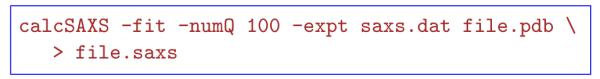
Use of the calcSAXS helper to calculate a SAXS curve given molecular structure file.pdb from the Unix command line. The file saxs.dat would contain SAXS data and −numQ 100 specifies that the SAXS curve is computed using 100 points in q spaced evenly over the interval of q values present in saxs.dat, while −fit specifies that the bound-solvent scattering contribution is calculated using a fit to the experimental SAXS data. The resulting scattering curve and residual (difference between observed and calculated scattering curves) is written to file.saxs.
3. Examples of use of SAXS, WAXS and SANS data
Here we review examples of the use of SASS data used together with NMR data for biomolecular structure determination. The first example illustrates how the addition of SAXS data can improve a structure determined using NMR data. In the remainder of the examples, the structure determination is made possible only with the use of SASS data.
3.1. Refinement of Lysozyme
This is an unpublished example which solely serves the purpose of illustrating how one can include SAXS/WAXS data in a standard Xplor-NIH structure calculation which employs a complete set of NMR data. While some of our results show improved Xplor-NIH metrics relative to previously deposited structures, being unfamiliar with the original NMR data, we are unable to truly evaluate the fit of that data to our structures. This complete example in contained in the Xplor-NIH distribution in the directory eginput/saxsref. The structure is that of hen egg white lysozyme, a 139 residue protein with four disulfide bonds. NMR data was taken from PDB entry 1E8L [23], while the SAXS/WAXS data was provided directly by Alex Grishaev (private communication).
The experimental NMR data comprised distance, dihedral and RDC restraints. There were 1631 NOE-derived and 60 hydrogen bond distance restraints, 43 of which were violated by more than 0.5 Å in the reference X-ray structure (PDB entry 193L [24]) and thus were omitted in our calculations for simplicity. We made use of 110 J-coupling-derived torsion angle restraints for ϕ and χ1 angles. Backbone amide RDC measurements were reported in two aligning media, and were included in our calculations with initial Da and rhombicity values taken to be those obtained by fitting to the deposited NMR structure. In our refinement calculations, additional energy terms included the knowledge-based potentials of mean force for torsion angles (torsionDB) [26] and hydrogen bonds (HBDB) [25], and standard Xplor-NIH covalent and nonbonded energy terms.
The refinement protocol started with the coordinates of model 49 of PDB entry 1E8L, the author-indicated representative structure. We present results for this structure separately in Table 1. Structure determination consisted of high-temperature torsion-angle dynamics at 3000 K, followed by torsion angle simulated annealing from 3000 K down to 25 K in increments of 12.5 K. Finally, gradient minimization was performed first in torsion-angle space, and then using Cartesian coordinates. The Da and rhombicity of the two alignment tensors were fixed to values computed from the deposited NMR structure until the Cartesian minimization step, where they were allowed to float to optimize the RDC fit. 100 structures were calculated and the 10 with the lowest energy structures were retained for analysis. Further details of the protocol can be obtained from the script available as described above.
Table 1.
Structure statics for Lysozyme refinement with and without SAXS data for the 10 lowest energy structures.
| all NMR data | deposited NMR | X-ray | ||
|---|---|---|---|---|
| Metric | without SAXS | with SAXS | Structures (1E8L) a | Structure |
| NOE violations b | 4.3 ±2.5 | 0.2 ±0.4 | 0.0±0.0 (0) | 0 |
| RDC R-factor, medium 1 (%) | 9.9 ±1.5 | 5.9 ±0.3 | 5.9±0.3 (5.9) | 13.3 |
| RDC R-factor, medium 2 (%) | 13.8 ±2.4 | 9.2 ±0.8 | 5.7±0.4 (5.8) | 15.2 |
| dihedral violations c | 4.4 ±1.2 | 0.1 ±0.3 | 0.0±0.2 (0) | 0 |
| SAXS χ2 | 2.3 ±1.4 | 0.4±0.1 | 1.7±0.6 (1.5) | 0.86 |
| HBDB energy (kcal/mol)d | −116.4 ±18.8 | −160.7 ±13.3 | −45.6±9.1 (−36.2) | −255.12 |
| torsionDB violations e | 3.8 ±2.6 | 1.4 ±1.5 | 1.7±0.9 (2) | 0 |
| bond violations | 6.5 ±5.2 | 0.4 ±0.8 | 0.0±0.0 (0) | 0 |
| angle violations | 8.6 ±5.9 | 0.1 ±0.3 | 10.3±0.8 (10) | 48 |
| improper violations | 3.1 ±2.7 | 0 ±0 | 0.0±0.0 (0) | 24 |
| bad nonbonded contacts f | 21.2 ±7.5 | 2.7 ±1.8 | 166.5±7.8 (176) | 48 |
| precision to mean (Å) g | 2.30±0.58 | 0.84±0.14 | 0.50±0.13 | − |
| acc. to NMR struct. (Å) h | 2.78±0.56 | 1.50±0.14 | 0.52±0.20 | 1.46 |
| acc. to X-ray struct. (Å) i | 2.82±0.59 | 1.32±0.19 | 1.48±0.10 (1.46) | − |
Results for all 50 of the deposited structures for PDB entry 1E8L. The numbers in parentheses show results for the author-identified representative model of this entry, model number 49.
Number of violations of NOE- or hydrogen-bond derived distance restraints greater than 0.5Å. 43 distance restraints from the deposited data were discarded as they are violated in the X-ray structure, leaving 1588 NOE-derived and 60 hydrogen bond-derived distance restraints in the structure calculation.
Number of dihedral violations of the 110 J-coupling-derived dihedral restraints violated by 5° or more.
Energy of Xplor-NIH’s knowledge-based HBDB term [25]. A lower number indicates the presence of more/better hydrogen bonds.
Number of torsionDB [26] energy terms with energies greater than those of 99.95% of the structures in the database of structures used to construct the term.
As reported by Xplor-NIH, the number of atom pairs whose distance is less than the sum of their respective van der Waals radii minus 0.2 Å.
The average root mean square distance (RMSD) of backbone atoms of each structure to the unregularized mean coordinates.
The average RMSD of backbone atoms to the representative NMR structure, model 49 of PDB entry 1E8L [23].
The average RMSD of backbone atoms to the X-ray structure, PDB entry 193L [24].
Figures 2 and 3, and Table 1 summarize the difference in structures calculated using solely NMR data to those calculated with a SAXS/WAXS restraint in addition to the NMR data. Striking is the improvement in convergence: all fit metrics reported in Table 1 are better fit when SAXS/WAXS data is included in the structure calculation. The bundle of structures is qualitatively tighter in Figure 2 and the SAXS/WAXS fit better, with less spread in Figure 3. Perhaps most importantly, the accuracy of the computed structures relative to the X-ray structure is greatly improved, from 2.8 to 1.3 Å. As in Reference [23], a better fit to the X-ray structure can be obtained if residues with poor precision are omitted from the calculations.
Figure 2.
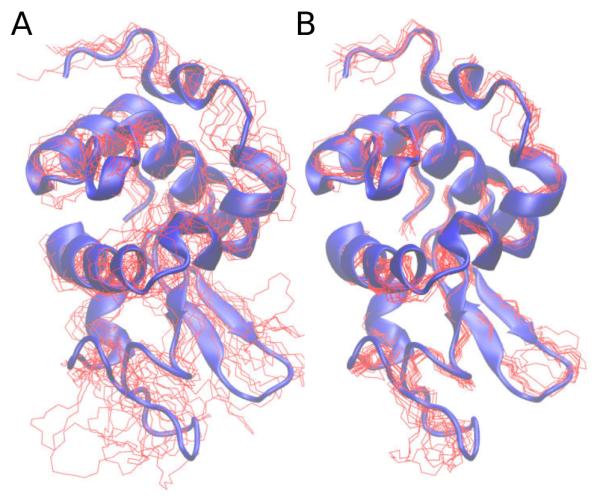
The structure of hen egg white lysozyme. Red lines depict backbone coordinates of the lowest energy 10 structures calculated omitting SAXS/WAXS data (Panel A) and including SAXS/WAXS data (panel B). Both calculations included NMR data [23]. The two panels contain a blue cartoon representation of the X-ray structure from PDB ID 193L [24].
Figure 3.

Comparison of SAXS/WAXS curves for hen egg white lysozyme. Panels A and B depict the agreement to experiment of the SAXS/WAXS curves associated with the 10 lowest energy structures calculated without and with SAXS/WAXS data, respectively. The experimental data is shown in black with gray vertical bars equal to 1 SD.; the curves calculated from the simulated annealing structures are shown in red. The residuals, given by , are plotted above each panel.
The statistics for the 50 NMR structures deposited in PDB entry 1E8L show very good convergence and precision relative to the current structures calculated without SAXS/WAXS data. This is likely due to the use of different refinement protocols and the use of different molecular parameters, as evidenced by the large number of non-bonded violations in the 1E8L structures reported in Table 1. A comprehensive analysis of the 1E8L restraints and systematic structure recalculation is outside the scope of this review. It should be noted that, while the use of SAXS/WAXS data has improved the local structure, such as the appearance of the α-helices when comparing panels A and B of Fig. 2, the scattering curve is rather insensitive to these features over the fitted q range, such that improvement is rather due to better convergence: the global minimum with all restraints satisfied is better sampled with the inclusion of SAXS/WAXS data.
3.2. Ensemble DNA Calculation using NMR and WAXS data
In this example, the Dickerson dodecamer DNA was studied by including a large number of NMR restraints, and WAXS data [7]. The NMR data comprised distance restraint, RDC, chemical shift anisotropy (CSA) and J-coupling data [27, 28]. The corresponding observables were calculated by proper averaging over the ensemble members. In addition to the experimental terms, we employed dihedral restraints corresponding to B-form DNA with very generous bounds, base-pair planarity restraints, and database restraints for residue-residue positioning [29] and torsion angles [30], in addition to standard covalent and nonbonded Xplor-NIH energy terms. To obtain good convergence of the multi-membered ensemble calculations, we found it necessary to restrain the inter-ensemble phosphorus atoms distance to 0.5 Å via a relative atom position restraint [31], and to employ multiple shape potential [31] terms to more directly restrict intraensemble rotation and shape changes of both the overall structure, and those corresponding to the central 6 base pairs. The structure calculation comprised high-temperature dynamics followed by a simulated annealing refinement starting with the coordinates of canonical B-form DNA.
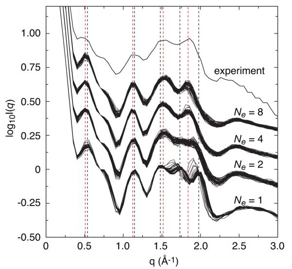
The NMR data were adequately satisfied by a single structure when the WAXS data was omitted [27], but the WAXS profile was found to be inconsistent with this structure [13]. However, using an ensemble representation [31] the NMR and WAXS data could be satisfied using an ensemble size Ne of 4. Qualitative examination of average structures (Fig, 4) computed for Ne = 1 and 4 shows that the Ne = 1 structure is compressed relative to the Ne = 4 structure. In the WAXS curve, this compression corresponds to a shift to larger values of the peak at q ~ 1.8 Å−1. Even when the X-ray target function was included, we found that a single structure could not fit the WAXS data adequately. As Figures 4-6 show, a good fit can be obtained by refining against the WAXS term and allowing the number of structures within the ensemble to increase to four.
Figure 4.
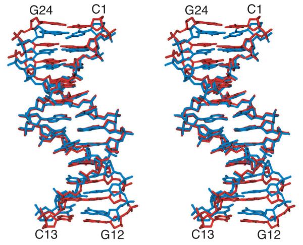
Stereoview showing a best-fit superposition of the regularized mean Ne = 1 (blue) and Ne = 4 (red) structures of the Dickerson dodecamer DNA. For Ne = 4, this structure is derived from the average ensemble structures for 50 ensembles. It is evident that single structure approximation is compressed relative to the Ne = 4 structures. This fact is reflected in the shift of the 4th peak in Fig. 5, and corresponds to capturing the correct basepair rise [13]. Adapted from Schwieters and Clore [7] published in Biochemistry (American Chemical Society) while the authors were U.S. Government employees at the National Institutes of Health.
Figure 6.
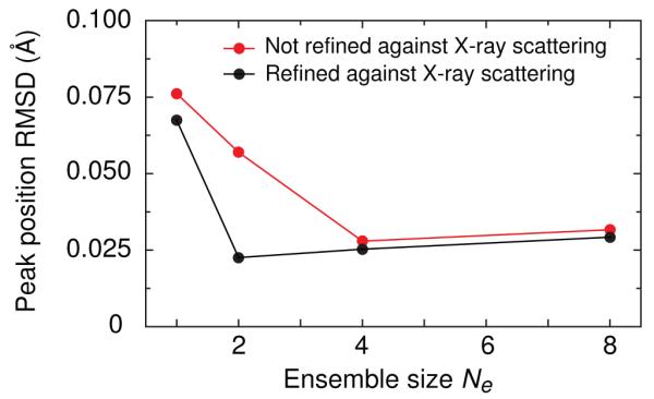
Comparison for the Dickerson dodecamer DNA of the 4 peak solution X-ray scattering peak position rms difference between observed and calculated values for Ne = 1, 2, 4, and 8 ensembles calculated with (black) and without (red) the X-ray scattering potential term in the refinement target function. For the Ne = 1 structures obtained without the X-ray scattering term, the first peak is absent and is therefore excluded from the rms deviation calculation for that point. Adapted from Schwieters and Clore [7] published in Biochemistry (American Chemical Society) while the authors were U.S. Government employees at the National Institutes of Health.
In addition to fitting the data, the ensemble representation allows us to probe dynamical aspects of the DNA structure, such as fraction population present in different ribose conformations, distributions of base-pair rise, relative populations of the BI and BII nucleic acid form structures, and expected order parameters corresponding to various bond-vector motion. See Ref. [31] for more details. This example is included in the Xplor-NIH distribution as a sample calculation in the eginput/dna_refi directory.
3.3. Rigid Body Docking: Enzyme I
In this example the structure of the 128 kDa Enzyme I homodimer was solved using RDCs and SAXS/WAXS data [18]. In the structure determination protocol the coordinates of the C-terminal dimerization domain were held fixed in space throughout to those determined by crystallography [32], a choice supported by the fact that the C-terminal domain is the same in all three existing crystal structures of EI from different species [33–35], as well as in the crystal structure of the isolated C-terminal domain [36]. The atomic coordinates of the 2 N-terminal domains were moved as rigid bodies corresponding to those determined by NMR [37], and the atoms in the linker region were given full degrees of freedom. The full protocol involved initial breaking of the linker and re-docking of the N-terminal domains back on to the C-terminal domain dimer such that all possible relative orientations would be allowed and that the RDC fit of the EIN domain of the dimer would be within a small tolerance of that determined from an isolated EIN domain. The linker was then reformed allowing only translation of the EIN domains such that the RDC fit would be maintained. The resulting structures contained multiple orientations of EIN relative to EIC due to the known degeneracy of RDC restraints [38]. Final rigid-body refinement was performed using SAXS/WAXS and RDC data. SAXS/WAXS data allowed the selection of the correct EIN/EIC orientation due to the fact that the lowest energy structures consistently took the published conformation. Results are shown in Figs. 7 and 8. The existing crystal structures did not fit RDC or SAXS data. Indeed, in the SAXS/WAXS+RDC EI structure determination, a small number of inter-domain contacts were found to stabilize the structure in solution. In this case, RDCs were essential to confirm that the N-terminal domain was in the conformation of the previously-determined solution structure, but by themselves they were not sufficient to determine the full structure of EI.
Figure 7.

Comparison of experimental SAXS/WAXS and SANS curves for free EI with the calculated curves for the simulated annealing structures obtained by refinement against the SAXS/WAXS and RDC data. (A) SAXS/ WAXS and (B) SANS. The experimental data is shown in black with gray vertical bars equal to 1 SD; the calculated curves for the final 100 simulated annealing structures are shown in red. The residuals, given by , are plotted above each panel. The structures were determined by fitting the SAXS/WAXS curve in the range q ≤ 0.44 Å−1, and the upper end of this range is indicated by the vertical dashed black line in panel A. Adapted from Schwieters et. al. [18] published in J. Am. Chem. Soc. (American Chemical Society) while the authors were U.S. Government employees at the National Institutes of Health.
Figure 8.
The structure of free EI determined from RDC and SAXS data. A best-fit superposition (to the EIC dimer which remains fixed) of the 100 final simulated annealing structures. The backbone (N, Cα , C’) atoms of the EIN domain are shown in blue, and the EIC domain is depicted as a ribbon diagram in red. Adapted from Schwieters et. al. [18] published in J. Am. Chem. Soc. (American Chemical Society) while the authors were U.S. Government employees at the National Institutes of Health.
Structures of Enzyme I complexed with HPr [18] and of a mutant version of Enzyme I [39] were also determined using this protocol. This example is included in the Xplor-NIH distribution as a sample calculation in the eginput/saxs_EI directory.
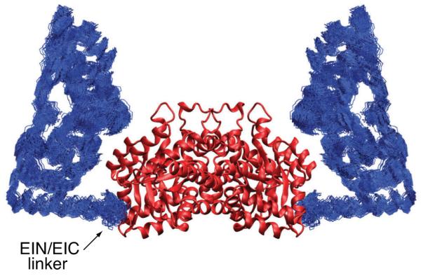
3.4. Rigid body Docking in the presence of large-amplitude motion: the full length HIV capsid protein
This example again represents a structure determination of a symmetric homodimer with C-terminal dimerization domains [22]. However, this problem is rather more involved due to two complicating factors: 1) the fact that a significant fraction of the molecules are monomeric at experimental conditions and 2) since the N- and C- terminal domains interact minimally, large amplitude motion of one relative to the other occurs such that a single-structure approximation is inappropriate and an ensemble representation becomes necessary. The structures of the two domains had been determined previously by crystallographic and NMR methods. The ratio of monomer to dimer was determined using analytical ultracentrifugation, while RDCs were initially used to confirm the structures of the two domains, to demonstrate that the domains align independently and to choose the proper structure of C-terminal dimer. The ensemble representation of the dimer required extension of the usual restraints used to preserve C2 symmetry of homodimers, because now the symmetry applies to the ensemble rather than to individual structures. Additionally, ensemble weights were allowed to vary to best fit observables, and reduce the minimal-required ensemble size.
Results are shown in Figures 9 and 10. The structure of the monomer was found to be strikingly different than that of the dimer due the fact that the monomer samples regions of space which are occluded by the dimerization partner, and that there are apparently important transient contacts between the N- and C-terminal domains in the monomer. These contacts are not possible in the dimer due to the presence of the dimerization partner.
Figure 9.

Structural ensembles calculated for the wild-type capsid (CAFL) dimer (A) and monomer (B). In panels A and B the C-terminal domain is displayed as light gray ribbons. In panel B the C-terminal domain of the monomer is displayed in the same orientation as that of the A subunit in panel B. The overall distribution of the N-terminal domain relative to the C-terminal domain is displayed as a reweighted atomic probability [40] plotted at 50% (blue) and 10% (transparent red) of maximum. Additionally, a single complete monomer structure is plotted in panel B (with the N-terminal domain depicted in green) which corresponds to one cluster of ensemble members which form transient contacts in the monomer and would be occluded in the dimer ensemble. Adapted from Deshmukh et. al. [22] published in J. Am. Chem. Soc. (American Chemical Society) while the authors were U.S. Government employees at the National Institutes of Health.
Figure 10.
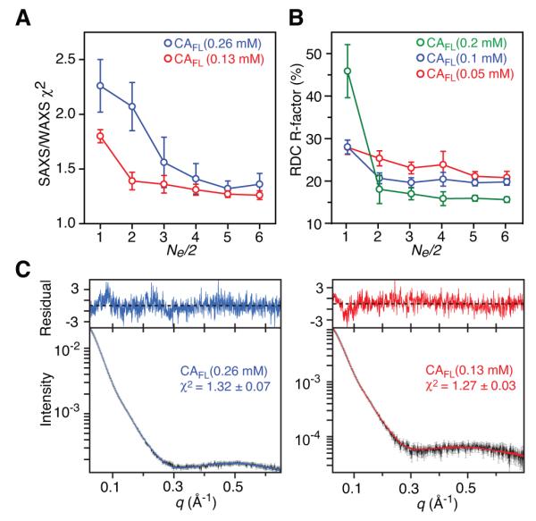
Fit to experimental SAXS/WAXS and RDC data for ensemble simulated annealing refinement of the wild-type capsid protein CAFL. Each ensemble comprises the same number of monomers and dimers (i.e. Ne = weighted according to their populations at different concentrations as determined by analytical ultracentrifugation [22]. (A) SAXS/WAXS χ2 as a function of ensemble size Ne/2. (B) C-terminal domain RDC R-factors as a function of ensemble size Ne/2. (C) Agreement between observed and calculated SAXS/WAXS curves. The experimental SAXS/WAXS data are shown in black with grey vertical bars equal to 1 s.d., and the calculated curves are shown in blue and red for the data at CAFL concentrations of 0.26 and 0.13 mM (in subunits), respectively. The residuals, given by , are plotted above the curves. Adapted from Deshmukh et. al. [22] published in J. Am. Chem. Soc. (American Chemical Society) while the authors were U.S. Government employees at the National Institutes of Health.
The calculations employed the SARDC potential [41] which calculates the alignment tensor from molecular shape as applicable for RDC experiments performed using a purely steric alignment medium such as neutral bicelles. In the time-scale regime considered in this example, each ensemble member has its own effective alignment tensor, and if one were to use the common practice of letting the alignment tensors float to optimize the fit to the experimental RDC data, the fit would be unstable and ill-determined as there would be far too many parameters for the given data.
For all structure calculations, the backbone atoms of the C-terminal domains were kept fixed and the backbone atoms of the N-terminal domains moved as rigid bodies, while atoms in the linker region (residues 146-149) were given all degrees of freedom. The ensemble members (both monomer and dimer) were allowed to move freely with respect to one another (i.e. while a van der Waals repulsion term prevented atomic overlap within each ensemble member, atomic overlap between different ensemble members is allowed since the ensemble reflects a population distribution). Sidechain atoms of the N- and C-terminal domains were given torsion angle degrees of freedom throughout.
All active torsion angles (including those in the linker region) were initially randomized uniformly in the range −8 … + 8° and an initial gradient minimization performed. This initial randomization and minimization was repeated until the number of nonbonded contacts between the N- and C- terminal domains was below a threshold value. This step was followed by a high-temperature molecular dynamics and simulated annealing with ramped force constants and a final gradient minimization.
This example will be included in the Xplor-NIH distribution in the subdirectory eginput/capsid.
3.5. Structure of a large RNA
Fang et. al [42] solved a large 233 nucleotide RNA structure comprising the HIV-1 Rev response element (RRE) without NMR data primarily using SAXS and secondary structure information in a novel protocol involving fitting a SAXS-generated atomic density map. This sort of structure determination is possible for RNA because the structures are predominately A-form duplexes and standard biochemical approaches exist for the determination of nucleic acid secondary structure. Additional biochemical and homology information were used for the confirmation of the basic topology of this RNA. Xplor-NIH was used in refinement of the structure, but not the initial fold determination, which utilized the G2G program [43].
The resulting structure is rather extended, taking the form of the letter “A” (Fig. 11). A functional region between the two legs of the A was identified as the binding site of a dimer of the Rev protein: known Rev binding sites are located on each leg, and the determined distance between the binding sites commensurate with the size of the Rev dimer.
Figure 11.
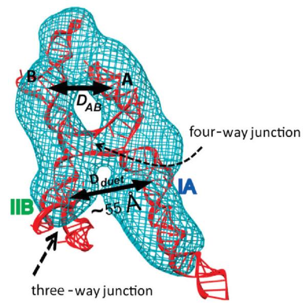
Determined structure of the RRE RNA (red) shown inside the SAXS/WAXS molecular envelope generated using the DAMMIN program [44] (blue). Various structural elements are indicated. The binding site of the Rev dimer is proposed to be between the legs IA and IIB at the arrow labeled Dduet. Adapted from Fang et. al. [42] published in Cell (Elsevier) while the authors were U.S. Government employees at the National Institutes of Health.
As a single conformation did not fit the SAXS data within experimental error, Xplor-NIH was also used to characterize the conformation space sampled by the RNA, with an ensemble of three equally weighted conformers chosen to best represent the data (Fig. 12). In this calculation the A-form duplexes were moved as rigid bodies rotating about bulges and junction regions of the RNA. The resulting ensemble member structures indicate that the distance between Rev binding sites has a standard deviation of 5 Å [42].
Figure 12.

Experimental SAXS/WAXS curve for the RRE RNA [42] with experimental error overlaid in black with 20 calculated SAXS/WAXS curves (blue) calculated from ensemble calculations employing three ensemble members. The inset shows the χ2 fit to experiment versus ensemble size. Adapted from Fang et. al. [42] published in Cell (Elsevier) while the authors were U.S. Government employees at the National Institutes of Health.
4. Concluding Remarks
We have seen that the complementary nature of SASS data relative to restraints derived from NMR data allows for an improvement of structure quality relative to that possible from NMR data alone. For single-domain proteins, the inclusion of SAXS/WAXS data with a full set of NMR data can significantly improve convergence and modestly improve structure accuracy. One can dock rigid-body domains using SAXS/WAXS combined with RDC data. For studies of molecular systems occupying multiple conformations SAXS/WAXS data have proven indispensable in structure determination. One of the reasons for this is the fact that SASS-derived restraints provide distance information which is a linear average over conformer structures. This is in contrast to the primary NMR source for distance information, data from NOE experiments, where ⟨r−6⟩−1/6 averaging overwhelmingly picks out the shortest possible inter-atomic distances, and provides very limited information about larger distances.
One approach for improving the fit of experimental SAXS curves to those calculated from molecular coordinates deserves mention here. In Reference [45], an alternate approach was taken for the treatment of the bound-solvent scattering contribution which at the same time refines the subtraction of background scattering (X-ray scattering in the absence of the sample). In that work the bound-solvent contribution was calculated using explicit water molecules, and as such, is likely not applicable in the context of structure calculation. However, the work identifies errors in background scattering subtraction as significantly reducing the quality of SASS fits, and a similar approach might be used within the context of the Xplor-NIH scattering implementation to achieve better fits to data, and more importantly, more accurate structures.
Finally, work is ongoing to advance the methodology used in the calculation of SAXS/WAXS curves. An approach similar to that used in the fast multipole method [46] employed for the calculation of Coulomb interactions has been developed [47]. This hierarchical approach should prove particularly important in applications to larger systems than those demonstrated here.
Highlights.
* We describe the use of SAXS, WAXS and SANS data in Xplor-NIH, along with NMR restraints.
* Instructions are given on how to include scattering data in Xplor-NIH scripts.
* We present five examples of the use of scattering data in structure calculations.
Figure 5.
Comparison of experimental and calculated solution X-ray scattering curves for the Dickerson dodecamer DNA. Curves from the best 50 ensembles for Ne values of 1, 2, 4, and 8 are displayed with an offset from the experimental scattering curve. Black and red vertical dashed lines represent the average peak positions for Ne = 1 and 4, respectively. While quantitative agreement with experiment was not obtained, peaks positions were accurately reproduced. Adapted from Schwieters and Clore [7] published in Biochemistry (American Chemical Society) while the authors were U.S. Government employees at the National Institutes of Health.
Acknowledgments
This work was supported by funds from the Intramural Program of the NIH, CIT (C.D.S.) and NIDDK (G.M.C.).
Glossary of Abbreviations
- SASS
Small Angle Solution Scattering
- SANS
Small Angle Neutron Scattering
- SAXS
Small Angle X-ray Scattering
- WAXS
Wide Angle X-ray Scattering
- RDC
Residual Dipolar Coupling
- SARDC
Sterically Aligned Residual Dipolar Coupling
Footnotes
Publisher's Disclaimer: This is a PDF file of an unedited manuscript that has been accepted for publication. As a service to our customers we are providing this early version of the manuscript. The manuscript will undergo copyediting, typesetting, and review of the resulting proof before it is published in its final citable form. Please note that during the production process errors may be discovered which could affect the content, and all legal disclaimers that apply to the journal pertain.
Acknowledgments The Xplor-NIH software package including example scripts is available online at http://nmr.cit.nih.gov.
Contributor Information
Charles D. Schwieters, Division of Computational Bioscience, Center for Information Technology, National Institutes of Health, Building 12A, Bethesda, MD 20892-5624
G. Marius Clore, Laboratory of Chemical Physics, National Institute of Diabetes and Digestive and Kidney Diseases, National Institutes of Health, Building 5, Bethesda, MD 20892-0510.
References
- [1].Clore GM, Gronenborn AM. Science. 1991;252:1390–1399. doi: 10.1126/science.2047852. [DOI] [PubMed] [Google Scholar]
- [2].Bax A. Prot. Science. 2003;12:1–16. doi: 10.1110/ps.0233303. [DOI] [PMC free article] [PubMed] [Google Scholar]
- [3].Koch MH, Vachette P, Svergun DI. Q. Rev. Biophys. 2003;36:147–227. doi: 10.1017/s0033583503003871. [DOI] [PubMed] [Google Scholar]
- [4].Hura GL, Menon AL, Hammel M, Rambo RP, Poole FL, II, Tsutakawa SE, Jenney FE, Jr, Classen S, Frankel KA, Hopkins RC, Yang Sung-jae, Scott JW, Dillard BD, Adams MWW, Tainer JA. Nature Methods. 2009;6:606–612. doi: 10.1038/nmeth.1353. [DOI] [PMC free article] [PubMed] [Google Scholar]
- [5].Grishaev A, Wu J, Trewheela J, Bax A. J. Am. Chem. Soc. 2005;127:16621–16628. doi: 10.1021/ja054342m. [DOI] [PubMed] [Google Scholar]
- [6].Chacon P, Moran F, Diaz JF, Pantos E, Andreu JM. Biophys. J. 1998;74:2760–2775. doi: 10.1016/S0006-3495(98)77984-6. [DOI] [PMC free article] [PubMed] [Google Scholar]
- [7].Schwieters CD, Clore GM. Biochemistry. 2007;46:1152–1166. doi: 10.1021/bi061943x. [DOI] [PubMed] [Google Scholar]
- [8].Gabel F, Simon B, Nilges M, Petoukhov M, Svergun D, Sattler M. J Biomol NMR. 2008;41:199–208. doi: 10.1007/s10858-008-9258-y. [DOI] [PubMed] [Google Scholar]
- [9].Schwieters CD, Kuszewski JJ, Tjandra N, Clore GM. J. Magn. Reson. 2003;160:66–74. doi: 10.1016/s1090-7807(02)00014-9. [DOI] [PubMed] [Google Scholar]
- [10].Schwieters CD, Kuszewski JJ, Clore GM. Progr. NMR Spectroscopy. 2006;48:47–62. [Google Scholar]
- [11].Fraser RDB, Macrae TP, Suzuki E. J. Appl. Crystallogr. 1978;11:693–694. [Google Scholar]
- [12].Svergun D, Barberato C, Koch MHJ. J. Appl. Cryst. 1995;28:768–773. [Google Scholar]
- [13].Zuo X, Tiede DM. J. Am. Chem. Soc. Comm. 2005;127:16–17. doi: 10.1021/ja044533+. [DOI] [PubMed] [Google Scholar]
- [14].Chacon P, Moran F, Diaz JF, Pantos E, Andreu JM. Biophys. J. 1998;74:2760–2775. doi: 10.1016/S0006-3495(98)77984-6. [DOI] [PMC free article] [PubMed] [Google Scholar]
- [15].Guo DY, Blessing RH, Langs DA. Acta Crystallogr. D, Biol. Crystallogr. 2000;56:1148–1155. doi: 10.1107/s0907444900008362. [DOI] [PubMed] [Google Scholar]
- [16].Saff EB, Kuijlaars ABJ. The Mathematical Intelligencer. 1997;19:5–11. [Google Scholar]
- [17].Svergun DI, Petoukhov MV, Koch MHJ. Biophys. J. 2001;80:2946–2953. doi: 10.1016/S0006-3495(01)76260-1. [DOI] [PMC free article] [PubMed] [Google Scholar]
- [18].Schwieters CD, Suh J-Y, Grishaev A, Ghirlando R, Takayama Y, Clore G. Marius. J. Am. Chem. Soc. 2010;132:13026–13045. doi: 10.1021/ja105485b. [DOI] [PMC free article] [PubMed] [Google Scholar]
- [19].Varshney A, Brooks FP, Wright WV. IEEE Comp. Graphics App. 1994;14:19–25. [Google Scholar]
- [20].Svergun DI, Richard S, Koch MHJ, Sayers Z, Kuprin S, Zaccai G. Proc. Natl. Acad. Sci. USA. 1998;95:2267–2272. doi: 10.1073/pnas.95.5.2267. [DOI] [PMC free article] [PubMed] [Google Scholar]
- [21].Press WH, Teukolsky SA, Vetterling WT, Flannery BP. Numerical Recipes in C. Cambridge U. Press; Cambridge: 1990. [Google Scholar]
- [22].Deshmukh L, Schwieters CD, Grishaev A, Ghirlando R, Baber JL, Clore GM. J. Am. Chem. Soc. 2013;135:16133–16147. doi: 10.1021/ja406246z. [DOI] [PMC free article] [PubMed] [Google Scholar]
- [23].Schwalbe H, Grimshaw SB, Spencer A, Buck M, Boyd J, Dobson CM, Redfield C, Smith LJ. Protein Sci. 2001;10:677–688. doi: 10.1110/ps.43301. [DOI] [PMC free article] [PubMed] [Google Scholar]
- [24].Vaney MC, Maignan S, Ries-Kautt M, Ducriux A. Acta Crystallogr. D. 1996;52:505–517. doi: 10.1107/S090744499501674X. [DOI] [PubMed] [Google Scholar]
- [25].Grishaev A, Bax A. J. Am. Chem. Soc. 2004;126:7281–7292. doi: 10.1021/ja0319994. [DOI] [PubMed] [Google Scholar]
- [26].Bermejo GA, Clore GM, Schwieters CD. Protein Science. 2012;21:1824–1836. doi: 10.1002/pro.2163. [DOI] [PMC free article] [PubMed] [Google Scholar]
- [27].Tjandra N, Tate S, Ono A, Kainosho M, Bax A. J. Am. Chem. Soc. 2000;122:6190–6200. [Google Scholar]
- [28].Wu Z, Delaglio F, Tjandra N, Zhurkin VB, Bax A. J. Biomol. NMR. 2003;26:297–315. doi: 10.1023/a:1024047103398. [DOI] [PubMed] [Google Scholar]
- [29].Kuszewski J, Schwieters CD, Clore GM. J. Am. Chem. Soc. 2001;123:3903–3918. doi: 10.1021/ja010033u. [DOI] [PubMed] [Google Scholar]
- [30].Clore GM, Kuszewski J. J. Am. Chem. Soc. 2003;125:1518–1525. doi: 10.1021/ja028383j. [DOI] [PubMed] [Google Scholar]
- [31].Clore GM, Schwieters CD. J. Am. Chem. Soc. 2004;126:2923–2938. doi: 10.1021/ja0386804. [DOI] [PubMed] [Google Scholar]
- [32].Teplyakov A, Lim K, Zhu PP, Kapadia G, Chen CC, Schwartz J, Howard A, Reddy PT, Peterkofsky A, Herzberg O. Proc. Natl. Acad. Sci. U.S.A. 2006;103:16218–16223. doi: 10.1073/pnas.0607587103. [DOI] [PMC free article] [PubMed] [Google Scholar]
- [33].Teplyakov A, Lim K, Zhu PP, Kapadia G, Chen CC, Schwartz J, Howard A, Reddy PT, Peterkofsky A, Herzberg O. Proc. Natl. Acad. Sci. U.S.A. 2006;103:16218–16223. doi: 10.1073/pnas.0607587103. [DOI] [PMC free article] [PubMed] [Google Scholar]
- [34].Oberholzer AE, Schneider P, Siebold C, Baumann U, Erni B. J. Biol. Chem. 2009;284:33169–33176. doi: 10.1074/jbc.M109.057612. [DOI] [PMC free article] [PubMed] [Google Scholar]
- [35].Marquez J, Reinelt S, Koch B, Engelmann R, Hengstenberg W, Scheffzek KJ. J. Biol. Chem. 2006;281:32508–32515. doi: 10.1074/jbc.M513721200. [DOI] [PubMed] [Google Scholar]
- [36].Oberholzer AE, Bumann M, Schneider P, Bachler C, Siebold C, Baumann U, Erni B. J. Mol. Biol. 2005;346:521–532. doi: 10.1016/j.jmb.2004.11.077. [DOI] [PubMed] [Google Scholar]
- [37].Garrett DS, Seok Y-J, Liao DT, Peterkofsky A, Gronenborn AM, Clore GM. Biochemistry. 1997;36:2517–2530. doi: 10.1021/bi962924y. [DOI] [PubMed] [Google Scholar]
- [38].Wang J, Walsh J, Kuszewski J, Wang YX. J. Magn. Res. 2007;189:90–103. doi: 10.1016/j.jmr.2007.08.018. [DOI] [PubMed] [Google Scholar]
- [39].Takayama Y, Schwieters CD, Grishaev A, Ghirlando R, Clore GM. J. Am. Chem. Soc. 2011;133:424–427. doi: 10.1021/ja109866w. [DOI] [PMC free article] [PubMed] [Google Scholar]
- [40].Schwieters CD, Clore GM. J. Biomol. NMR. 2002;23:221–225. doi: 10.1023/a:1019875223132. [DOI] [PubMed] [Google Scholar]
- [41].Huang J.-r., Grzesiek S. J. Am. Chem. Soc. 2010;132:694–705. doi: 10.1021/ja907974m. [DOI] [PubMed] [Google Scholar]
- [42].Fang Xianyang, Wang Jinbu, O’Carroll IP, Zuo M. Mitchell Xiaobing, Yu Yi Wang Ping, Liu Yu, Rausch JW, Dyba MA, Kjems J, Schwieters CD, Seifert S, Winans RE, Watts NR, Stahl SJ, Wingfield PT, Byrd RA, Le Grice SFJ, Rein A, Wang Yun-Xing. Cell. 2013;155:594–605. doi: 10.1016/j.cell.2013.10.008. [DOI] [PMC free article] [PubMed] [Google Scholar]
- [43].Wang J, Zuo X, Yu P, Xu H, Starich MR, Tiede DM, Shapiro BA, Schwieters CD, Wang YX. J. Mol. Biol. 2009;393:717–734. doi: 10.1016/j.jmb.2009.08.001. [DOI] [PMC free article] [PubMed] [Google Scholar]
- [44].Svergun DI. Biophys. J. 1999;76:2879–2886. doi: 10.1016/S0006-3495(99)77443-6. [DOI] [PMC free article] [PubMed] [Google Scholar]
- [45].Grishaev A, Guo LA, Irving T, Bax A. J. Am. Chem. Soc. 2010;132:15484–15486. doi: 10.1021/ja106173n. [DOI] [PMC free article] [PubMed] [Google Scholar]
- [46].Greengard L, Rokhlin V. J. Comput. Phys. 1987;73:325–348. [Google Scholar]
- [47].Gumerov NA, Berlin K, Fushman D, Duraiswami R. J. Comp. Chem. 2012;33:1981–1996. doi: 10.1002/jcc.23025. [DOI] [PMC free article] [PubMed] [Google Scholar]