Abstract
Motivation: As a promising tool for dissecting the genetic basis of complex traits, expression quantitative trait loci (eQTL) mapping has attracted increasing research interest. An important issue in eQTL mapping is how to effectively integrate networks representing interactions among genetic markers and genes. Recently, several Lasso-based methods have been proposed to leverage such network information. Despite their success, existing methods have three common limitations: (i) a preprocessing step is usually needed to cluster the networks; (ii) the incompleteness of the networks and the noise in them are not considered; (iii) other available information, such as location of genetic markers and pathway information are not integrated.
Results: To address the limitations of the existing methods, we propose Graph-regularized Dual Lasso (GDL), a robust approach for eQTL mapping. GDL integrates the correlation structures among genetic markers and traits simultaneously. It also takes into account the incompleteness of the networks and is robust to the noise. GDL utilizes graph-based regularizers to model the prior networks and does not require an explicit clustering step. Moreover, it enables further refinement of the partial and noisy networks. We further generalize GDL to incorporate the location of genetic makers and gene-pathway information. We perform extensive experimental evaluations using both simulated and real datasets. Experimental results demonstrate that the proposed methods can effectively integrate various available priori knowledge and significantly outperform the state-of-the-art eQTL mapping methods.
Availability: Software for both C++ version and Matlab version is available at http://www.cs.unc.edu/∼weicheng/.
Contact: weiwang@cs.ucla.edu
Supplementary information: Supplementary data are available at Bioinformatics online.
1 INTRODUCTION
Expression quantitative trait loci (eQTL) mapping aims at identifying single nucleotide polymorphisms (SNPs) that influence the expression level of genes. It has been widely applied to dissect genetic basis of complex traits (Bochner, 2003; Michaelson et al., 2009). Several important issues need to be considered in eQTL mapping. First, the number of SNPs is usually much larger than the number of samples (Tibshirani, 1996). Second, the existence of confounding factors, such as expression heterogeneity, may result in spurious associations (Listgarten et al., 2010). Third, SNPs (and genes) usually work together to cause variation in complex traits (Michaelson et al., 2009). The interplay among SNPs and the interplay among genes can be represented as networks and used as prior knowledge (Musani et al., 2007; Pujana et al., 2007). However, such prior knowledge is far from being complete and may contain a lot of noises. Developing effective models to address these issues in eQTL studies has recently attracted increasing research interests (Biganzoli et al., 2006; Kim and Xing, 2012; Lee and Xing, 2012; Lee et al., 2010).
In eQTL studies, two types of networks can be utilized. One is the genetic interaction network (Charles Boone and Andrews, 2007). Modeling genetic interaction (e.g. epistatic effect between SNPs) is essential to understanding the genetic basis of common diseases, since many diseases are complex traits (Lander, 2011). Another type of network is the network among traits, such as the protein–protein interaction (PPI) network or the gene co-expression network. Interacting proteins or genes in a PPI network are likely to be functionally related, i.e. part of a protein complex or in the same biological pathway (von Mering et al., 2002). Effectively utilizing such prior network information can significantly improve the performance of eQTL mapping (Lee and Xing, 2012; Lee et al., 2010).
Figure 1 shows an example of eQTL mapping with prior network knowledge. The interactions among SNPs and genes are represented by matrices S and G, respectively. The goal of eQTL mapping is to infer associations between SNPs and genes represented by the coefficient matrix W. Suppose that SNP ② is strongly associated with gene Ⓒ. Using the network prior, the moderate association between SNP ① and gene Ⓐ may be identified since ① and and Ⓒ have interactions.
Fig. 1.
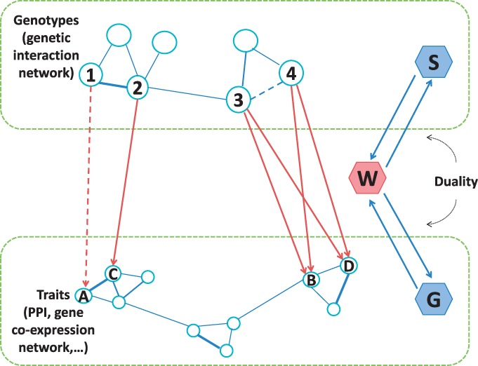
Examples of prior knowledge on genetic-interaction network S and gene–gene interactions represented by PPI network or gene co-expression network G. W is the regression coefficients to be learned
To leverage the network prior knowledge, several methods based on Lasso have been proposed (Biganzoli et al., 2006; Kim and Xing, 2012; Lee and Xing, 2012; Lee et al., 2010). In Biganzoli et al. (2006), the group-Lasso penalty is applied to model the genetic interaction network. In (Kim and Xing, 2012) and (Lee et al., 2010), the authors consider groupings of genes and apply a multi-task Lasso penalty. In (Lee and Xing, 2012), the authors further extend the model to consider grouping information of both SNPs and genes. These methods apply a ‘hard’ clustering of SNPs (genes) so that a SNP (gene) cannot belong to multiple groups. However, a SNP may affect multiple genes and a gene may function in multiple pathways. To address this limitation, in (Jenatton et al., 2011), the authors develop a model allowing overlap between different groups.
Despite their success, there are three common limitations of these group penalty based approaches. First, a clustering step is usually needed to obtain the grouping information. To address this limitation, (Kim and Xing, 2009; Li and Li, 2008) introduce a network-based fusion penalty on the genes. However, this method does not consider the genetic-interaction network. A two-graph-guided multi-task Lasso approach is developed in (Chen et al., 2012) to make use of gene co-expression network and SNP-correlation network. However, this method does not consider the network prior knowledge. The second limitation of the existing methods is that they do not take into consideration the incompleteness of the networks and the noise in them (von Mering et al., 2002). For example, PPI networks may contain false interactions and miss true interactions (von Mering et al., 2002). Directly using the grouping penalty inferred from the noisy and partial prior networks may introduce new bias and thus impair the performance. Third, in addition to the network information, other prior knowledge, such as location of genetic markers and gene-pathway information are also available. The existing methods cannot incorporate such information.
To address the limitations of the existing methods, we propose a novel approach, Graph-regularized Dual Lasso (GDL), which simultaneously learns the association between SNPs and genes and refines the prior networks. To support ‘soft’ clustering (allowing genes and SNPs to be members of multiple clusters), we adopt the graph regularizer to encode structured penalties from the prior networks. The penalties encourage the connected nodes (SNPs/genes) to have similar coefficients. This enables us to find multiple-correlated genetic markers with pleiotropic effects that affect multiple-correlated genes jointly. To tackle the problem of noisy and incomplete prior networks, we exploit the duality between learning the associations and refining the prior networks to achieve smoother regularization. That is, learning regression coefficients can help to refine the prior networks, and vice versa. For example, in Figure 1, if SNPs ③ and ④ have strong associations with the same group of genes, they are likely to have interaction, which is not captured in the prior network. An ideal model should allow to update the prior network according to the learned regression coefficients. GDL can also incorporate other available prior knowledge such as the physical location of SNPs and biology pathways to which the genes belong. The resultant optimization problem is convex and can be efficiently solved by using an alternating minimization procedure. We perform extensive empirical evaluation of the proposed method using both simulated and real eQTL datasets. The results demonstrate that GDL is robust to the incomplete and noisy prior knowledge and can significantly improve the accuracy of eQTL mapping compared to the state-of-the-art methods.
2 BACKGROUND: LINEAR REGRESSION WITH GRAPH REGULARIZER
Throughout the article, we assume that, for each sample, the SNPs and genes are represented by column vectors. Important notations are listed in Table 1. Let represent the K SNPs in the study, where is a random variable corresponding to the i-th SNP (e.g. 0, 1, 2 may encode the homozygous major allele, heterozygous allele and homozygous minor allele, respectively). Let represent expression levels of the N genes in the study, where zj is a continuous random variable corresponding to the j-th gene. The traditional linear regression model for association mapping between x and z is
| (1) |
where z is a linear function of x with coefficient matrix W and μ is an translation factor vector. And ϵ is the additive noise of Gaussian distribution with zero-mean and variance where γ is a scalar. That is, .
Table 1.
Summary of notations
| Symbols | Description |
|---|---|
| K | Number of SNPs |
| N | Number of genes |
| D | Number of samples |
| The SNP matrix data | |
| The gene matrix data | |
| A low-rank matrix | |
| The input affinity matrices of the genetic-interaction network | |
| The input affinity matrices of the network of traits | |
| The refined affinity matrices of the genetic-interaction network | |
| The refined affinity matrices of the network of traits | |
| The coefficient matrix to be inferred | |
| The graph regularizer from the genetic-interaction network | |
| The graph regularizer from the PPI network | |
| A non-negative distance measure |
The question now is how to define an appropriate objective function over W that (i) can effectively incorporate the prior network knowledge, and (ii) is robust to the noise and incompleteness in the prior knowledge. Next, we first briefly review Lasso and its variations and then introduce the proposed GDL method.
2.1 Lasso and LORS
Lasso (Tibshirani, 1996) is a method for estimating the regression coefficients W using penalty for sparsity. It has been widely used for association mapping problems. Let be the SNP matrix and be the gene-expression matrix. Each column of X and Z stands for one sample. The objective function of Lasso is
| (2) |
where denotes the Frobenius norm, is the -norm, is an vector of all 1’s, η is the empirical parameter for the penalty and is the parameter (also called weight) matrix parameterizing the space of linear functions mapping from X to Z.
Confounding factors, such as unobserved covariates, experimental artifacts and unknown environmental perturbations, may mask real signals and lead to spurious findings. LORS (Yang et al., 2013) uses a low-rank matrix to account for the variations caused by hidden factors. The objective function of LORS is
| (3) |
where is the nuclear norm, η is the empirical parameter for the penalty to control the sparsity of W and λ is the regularization parameter to control the rank of L. L is a low-rank matrix assuming that there are only a small number of hidden factors influencing the gene-expression levels.
2.2 Graph-regularized Lasso
To incorporate the network prior knowledge, group sparse Lasso (Biganzoli et al., 2006), multi-task Lasso (Obozinski and Taskar, 2006) and SIOL(Lee and Xing, 2012) have been proposed. Group sparse Lasso makes use of grouping information of SNPs; multi-task Lasso makes use of grouping information of genes, while SIOL uses information from both networks. A common drawback of these methods is that the number of groups (SNP and gene clusters) has to be predetermined. To overcome this drawback, we propose to use two graph regularizers to encode the prior network information. Compared with the previous group penalty-based methods, our method does not need to pre-cluster the networks and thus may obtain smoother regularization. Moreover, these methods do not consider confounding factors that may mask real signals and lead to spurious findings. In this article, we further incorporate the idea in LORS (Yang et al., 2013) to tackle the confounding factors simultaneously.
Let  and
and  be the affinity matrices of the genetic interaction network (e.g. epistatic effect between SNPs) and network of traits (e.g. PPI network or gene co-expression network), and
  and
and  be their degree matrices. Given the two networks, we can employ a pairwise comparison between
  and
and  if SNPs i and j are closely related,
  is small. The pairwise comparison can be naturally encoded in the weighted fusion penalty
 This penalty will enforce
  for closely related SNP pairs (with large
  value). Then, the graph regularizer from the genetic-interaction network takes the following form
 |
(4) |
Similarly, the graph regularizer for the network of traits is
| (5) |
These two regularizers encourage the connected nodes in a graph to have similar coefficients. A heavy penalty occurs if the learned-regression coefficients for neighboring SNPs (genes) are disparate. and are known as the combinatorial graph Laplacian, which are positive semi-definite (Chung, 1997). Graph-regularized Lasso (G-Lasso) solves the following optimization problem
 |
(6) |
where are regularization parameters.
3 GDL
In eQTL studies, the prior knowledge is usually incomplete and contains noise. It is desirable to refine the prior networks according to the learned regression coefficients. There is a between the prior networks and the regression coefficients: learning coefficients can help to refine the prior networks, and vice versa. This leads to mutual reinforcement when learning the two parts simultaneously.
Next, we introduce the GDL. We further relax the constraints from the prior networks (two graph regularizers) introduced in Section 2.2, and integrate the G-Lasso and the dual refinement of graphs into a unified objective function
 |
(7) |
where are positive parameters controlling the extent to which the refined networks should be consistent with the original prior networks. and are the degree matrices of S and G. Note that the objective function considers the non-negativity of S and G. As an extension, the model can be easily extended to incorporate prior knowledge from multiple sources. We only need to revise the last two terms in Equation (7) to where f and e are the number of sources for genetic interaction networks and gene trait networks, respectively.
3.1 Optimization: an alternating minimization approach
In this section, we present an alternating scheme to optimize the objective function in Equation (7) based on block coordinate techniques. We divide the variables into three sets: {L}, {S, G} and We iteratively update one set of variables while fixing the other two sets. This procedure continues until convergence. Since the objective function is convex, the algorithm will converge to a global optima. The optimization process is as follows. The detailed algorithm is included in the Supplementary Material (Algorithm 1).
(1) While fixing optimize using singular value decomposition (SVD).
Lemma 3.1 —
(Mazumder et al., 2010) Suppose that matrix A has rank r. The solution to the optimization problem
(8) is given by where with is the Singular Value Decomposition (SVD) of , and
Thus, for fixed the formula for updating L is
| (9) |
(2) While fixing optimize using semi-non-negative matrix factorization (semi-NMF) multiplicative updating on S and G iteratively (Ding et al., 2010). For the optimization with non-negative constraints, our updating rule is based on the following two theorems. The proofs of the theorems are given in Section 3.2.
Theorem 3.2 —
For fixed and G, updating S according to Equation (10) monotonically decreases the value of the objective function in Equation (7) until convergence.
(10) where is a matrix of all 1’s. are element-wise operators. Since may take mixed signs, we denote where and
Theorem 3.3. —
For fixed and S, updating G according to Equation (11) monotonically decreases the value of the objective function in Equation (7) until convergence.
(11) where is an matrix of all 1’s.
The above two theorems are derived from the Karush–Kuhn–Tucker (KKT) complementarity condition (Boyd and Vandenberghe, 2004). We show the updating rule for S below. The analysis for G is similar and omitted. We first formulate the Lagrange function of S for optimization
| (12) |
The partial derivative of the Lagrange function with respect to S is
| (13) |
Using the KKT complementarity condition for the non-negative constraint on S, we have
| (14) |
The above formula leads to the updating rule for S in Equation (10). It has been shown that the multiplicative updating algorithm has first order convergence rate (Ding et al., 2010).
(3) While fixing optimize using the coordinate descent algorithm.
Because we use the penalty on W, we can use the coordinate descent algorithm for the optimization of W, which gives the following updating formula:
| (15) |
where and
 |
(16) |
The solution of updating μ can be derived by setting which gives
| (17) |
3.2 Convergence analysis
In the following, we investigate the convergence of the algorithm. First, we study the convergence for the second step. We use the auxiliary-function approach (Lee and Seung, 2000) to analyze the convergence of the multiplicative updating formulas. Here we first introduce the definition of auxiliary function.
Definition 3.4 —
Given a function L(h) of any parameter h, a function is an auxiliary function for L(h) if the conditions
(18) are satisfied for any given (Lee and Seung, 2000).
Lemma 3.5 —
If Z is an auxiliary function for function L(h), then L(h) is non-increasing under the update (Lee and Seung, 2000).
(19)
Theorem 3.6 —
Let denote the Lagrange function of S for optimization. The following function
(20) is an auxiliary function for Furthermore, it is a convex function in S and its global minimum is
(21)
Theorem 3.6 —
can be proved using a similar idea to that in (Ding et al., 2006) by validating (i) (ii) (iii) is convex with respect to S. The formal proof is provided in the Supplementary Material.
Theorem 3.7 —
Updating S using Equation (10) will monotonically decrease the value of the objective in Equation (7), the objective is invariant if and only if S is at a stationary point.
Proof —
By Lemma 3.5 and Theorem 3.6, for each subsequent iteration of updating S, we have . Thus monotonically decreases. Since the objective function Equation (7) is obviously bounded below, the correctness of Theorem 3.2 is proved. Theorem 3.3 can be proved similarly. □
In addition to Theorem 3.7, since the computation of L in the first step decreases the value of the objective in Equation (7), and the coordinate descent algorithm for updating W in the third step also monotonically decreases the value of the objective, the algorithm is guaranteed to converge.
4 GENERALIZED GDL
In this section, we extend our model to incorporate additional prior knowledge such as SNP locations and biological pathways. If the physical locations of two SNPs are close or two genes belong to the same pathway, they are likely to have interactions. Such information can be integrated to help refine the prior networks.
Continue with our example in Figure 1. If SNPs ③ and ④ affect the same set of genes (Ⓑ and Ⓓ), and at the same time, they are close to each other, then it is likely there exists interaction between ③ and ④.
Formally, we would like to solve the following optimization problem
 |
(22) |
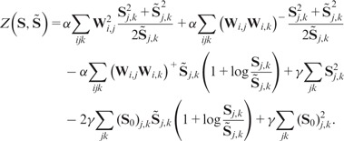
Here is a non-negative distance measure. Note that the Euclidean distance is used in previous sections. S and G are initially given by inputs and We refer to this generalized model as the generalized GDL (GGDL). GGDL executes the following two steps iteratively until the termination condition is met: (i) update W while fixing S and G and (ii) update S and G according to W, while guarantee that both  and
and  decrease.
These two steps are based on the aforementioned duality between learning W and refining S and G. The detailed algorithm is provided in the Supplementary Material. Next, we illustrate the updating process assuming that S and G are unweighted graphs. It can be easily extended to weighted graphs.
Step 1 can be done by using the coordinate decent algorithm. In Step 2, to guarantee that both  and
and 
 decrease, we can maintain a fixed number of 1’s in S and G. Taking G as an example, once is selected to change from 0 to 1, another element with should be changed from 1 to 0.
The selection of (i, j) and is based on the ranking of (). Specifically, we examine κ pairs (the choice of κ depends on the user’s belief in the quality of the prior network. For example, it can be 5% of all (i, j) pairs) with the smallest distances. Among them, we pick those having no edges in G. Let be this set of pairs. Accordingly, we examine κ pairs with the largest distances. Among these pairs, we pick up only those having an edge in G. Let be this set of pairs. The elements of G corresponding to pairs in are candidates for updating from 0 to 1, since these pairs of genes are associated with similar SNPs. Similarly, elements of G corresponding to pairs in are candidates for updating from 1 to 0.
In this process, the prior knowledge of gene pathways can be easily incorporated to better refine G. For instance, we can further require that only the gene pairs in belonging to the same pathway are eligible for updating, and only the gene pairs in belonging to different pathways are eligible for updating. We denote the set of gene pairs eligible for updating by and respectively. Then, we choose pairs in set with smallest () and update from 0 to 1. Similarly, we choose pairs in set with largest () and update from 1 to 0.
Obviously, all ’s are smaller than if Thus,  is guaranteed to decrease. The updating process for S is similar except that we compare columns rather than rows of W and use SNP locations rather than pathway information for evaluating the eligibility for updating. The updating process ends when no such pairs can be found so that switching their values will result in a decrease of the objective function.
The convergence of GGDL can be observed as follows. The decrease of the objective function value in the first step is straightforward since we minimize it using coordinate decent. In the second step, the change of the objective function value is given by
| (23) |
which is always negative. Thus, in each iteration, the objective function value decreases. Since the objective function is non-negative, the process eventually converges.
Theorem 4.1 —
GGDL converges to the global optimum if both
and
are convex to W.
Proof: —
The last two terms in Equation (22) are linear with respect to S and G, and convex to W according to the conditions listed. Thus the objective function is convex over all variables. A convergent result to the global optimum can be guaranteed. □
5 EXPERIMENTS
In this section, we perform extensive experiments to evaluate the performance of the proposed methods. We use both simulated datasets and real yeast eQTL dataset (Brem et al., 2005). For comparison, we select several state-of-the-art methods, including SIOL (Lee and Xing, 2012), two graph guided multi-task lasso (mtlasso2G) (Chen et al., 2012), sparse group Lasso (Biganzoli et al., 2006), sparse multi-task Lasso (Biganzoli et al., 2006), LORS (Yang et al., 2013) and Lasso (Tibshirani, 1996). For all the methods, the tuning parameters were learned using cross validation.
5.1 Simulation study
We first evaluate the performance of the selected methods using simulation study. Note that GGDL requires additional prior knowledge and will be evaluated using real dataset.
We adopt the same setup for the simulation study as that in (Lee and Xing, 2012; Yang et al., 2013) and generate synthetic datasets as follows. 100 SNPs are randomly selected from the yeast eQTL dataset (Brem et al., 2005) (112 samples). Ten gene-expression profiles are generated by (), where () denotes Gaussian noise. is used to model non-genetic effects, which is drawn from , where . Σ is generated by , where and C is the number of hidden factors and is set to 10 by default. The association matrix W is generated as follows. Three sets of randomly selected four SNPs are associated with three gene clusters (1–3), (4–6), (7–10), respectively. In addition, one SNP is associated with two gene clusters (1–3) and (4–6), and one SNP is associated with all genes. The association strength is set to 1 for all selected SNPs. The clustering structures among SNPs and genes serve as the ground truth of the prior network knowledge. Only two of the three SNP (gene) clusters are used in W to simulate incomplete prior knowledge.
Figure 2 shows the estimated W matrix by various methods. The x-axis represents traits (1–10) and y-axis represents SNPs (1–100). From the figure, we can see that GDL is more effective than G-Lasso. This is because the dual refinement enables more robust model. G-Lasso outperforms SIOL and mtlasso2G, indicating that the graph regularizer provides a smoother regularization than the hard clustering based penalty. In addition, SIOL and mtlasso2G do not consider confounding factors. SIOL and mtlasso2G outperform multi-task Lasso and sparse group Lasso since it uses both SNP and gene grouping information, while multi-task Lasso and sparse group Lasso only use one of them. We also observe that all methods utilizing prior grouping knowledge outperform LORS and Lasso which cannot incorporate prior knowledge. LORS outperforms Lasso since it considers the confounding factors.
Fig. 2.
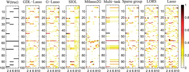
Ground truth of matrix W and that estimated by different methods. The x-axis represents traits and y-axis represents SNPs. Normalized absolute values of regression coefficients are used. Darker color implies stronger association
The ground-truth networks, prior networks and GDL-refined networks are shown in Figure 3. Note that only a portion of the ground-truth networks are used as prior networks. In particular, the information related to gene cluster (7–10) is missing in the prior networks. We observe that the refined matrix G well captures the missing grouping information of gene cluster (7–10). Similarly, many missing pairwise relationships in S are recovered in the refined matrix (points in red ellipses).
Fig. 3.
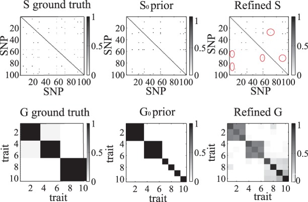
The ground truth networks, prior partial networks and the refined networks
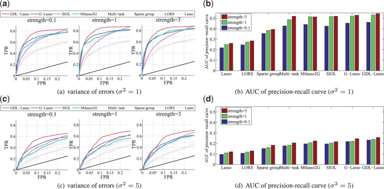
Using 50 simulated datasets with different Gaussian noise ( and we compare the proposed methods with alternative state-of-the-art approaches. For each setting, we use 30 samples for test and 82 samples for training. We report the averaged result from 50 realizations. Figure 4 shows the ROC curves of TPR-FPR for performance comparison, together with the areas under the precision-recall curve (AUCs) (Chen et al., 2012). The association strengths between SNPs and genes are set to be 0.1, 1 and 3, respectively. It is clear that GDL outperforms all alternative methods by effectively using and refining the prior network knowledge. We also computed test errors. On average, GDL achieved the best test error rate of 0.9122, and the order of the other methods in terms of the test errors is: G-Lasso (0.9276), SIOL (0.9485), Mtlasso2G (0.9521), Multi-task Lasso (0.9723), Sparse group Lasso (0.9814), LORS (1.0429) and Lasso (1.2153).
Fig. 4.
Power curves for synthetic data. The left plots show the ROC curve, where our model GDL achieved maximum power. The black solid line denotes what random guessing would have achieved. The right plots illustrate the areas under the precision-recall curve (AUCs) of different methods
To evaluate the effectiveness of dual refinement, we compare GDL and G-Lasso since the only difference between these two methods is whether the prior networks are refined during the optimization process. We add noises to the prior networks by randomly shuffling the elements in them. Furthermore, we use the signal-to-noise ratio defined as (Yang et al., 2013) to measure the noise ratio in the eQTL datasets. Here, we fix and use different σ’s to control SNR.
Figure 5 shows the results for different SNRs. For a fixed SNR, we vary the percentage of noises in the prior networks and compare the performance of selected methods. From the results, we can see that G-Lasso is more sensitive to noises in the prior networks than GDL is. Moreover, when the SNR is low, the advantage of GDL is more prominent. These results indicate using dual refinement can dramatically improve the accuracy of the identified associations.
Fig. 5.
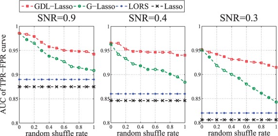
The areas under the TPR-FPR curve (AUCs) of Lasso, LORS, G-Lasso and GDL. In each panel, we vary the percentage of noises in the prior networks and
5.2 Yeast eQTL study
We apply the proposed methods to a yeast (Saccharomyces cerevisiae) eQTL dataset of 112 yeast segregants generated from a cross of two inbred strains (Brem et al., 2005). The dataset originally includes expression profiles of 6229 gene-expression traits and genotype profiles of 2956 SNPs. After removing SNPs with >10% missing values and merging consecutive SNPs high linkage disequilibrium, we get 1017 SNPs with unique genotypes (Huang et al., 2009). After removing the ones with missing values, 4474 expression profiles are selected. The genetic interaction network is generated as in (Lee and Xing, 2012). We use the PPI network downloaded from BioGRID (http://thebiogrid.org/) to represent the prior network among genes. It takes ∼1 day for GGDL, and ∼10 h for GDL to run into completion.
5.2.1 cis- and trans-enrichment analysis
We follow the standard cis-enrichment analysis (Listgarten et al., 2010) to compare the performance of two competing models. The intuition behind cis-enrichment analysis is that more cis-acting SNPs are expected than trans-acting SNPs. A two-step procedure is used in the cis-enrichment analysis (Listgarten et al., 2010): (i) for each model, we apply a one-tailed Mann–Whitney test on each SNP to test the null hypothesis that the model ranks its cis hypotheses no better than its trans hypotheses, (ii) for each pair of models compared, we perform a two-tailed paired Wilcoxon sign-rank test on the P-values obtained from the previous step. The null hypothesis is that the median difference of the P-values in the Mann–Whitney test for each SNP is zero. The trans-enrichment is implemented using similar strategy (Brem et al., 2003), in which genes regulated by transcription factors (obtained from http://www.yeastract.com/download.php) are used as trans-acting signals.
In addition to the methods evaluated in the simulation study, GGDL is also evaluated here (with ) (for GDL, The Euclidean distance is used as the distance metric. We rank pairs of SNPs and genes according to the learned W. S is refined if the locations of the two SNPs are <500 bp. G is refined if the two genes are in the same pathway. The pathway information is downloaded from Saccharomyces Genome Database [SGD (http://www.yeastgenome.org/)].
The results of pairwise comparison of selected models are shown in Table 2. In this table, a P-value shows how significant a method on the left column outperforms a method in the top row in terms of cis and trans enrichments. We observe that the proposed GGDL and GDL have significantly better enrichment scores than the other models. By incorporating genomic location and pathway information, GGDL performs better than GDL with P-value < 0.0001. The effectiveness of the dual refinement on prior graphs is demonstrated by GDL’s better performance over G-Lasso. Note that the performance ranking of these models is consistent with that in the simulation study.
Table 2.
Pairwise comparison of different models using cis-enrichment and trans-enrichment analysis
| GDL | G-Lasso | SIOL | Mtlasso2G | Multi-task | Sparse group | LORS | Lasso | |
|---|---|---|---|---|---|---|---|---|
| Cis-enrichment | ||||||||
| GGDL | 0.0003 | <0.0001 | <0.0001 | <0.0001 | <0.0001 | <0.0001 | <0.0001 | <0.0001 |
| GDL | – | 0.0009 | <0.0001 | <0.0001 | <0.0001 | <0.0001 | <0.0001 | <0.0001 |
| G-Lasso | – | – | <0.0001 | <0.0001 | <0.0001 | <0.0001 | <0.0001 | <0.0001 |
| SIOL | – | – | – | 0.1213 | 0.0331 | 0.0173 | <0.0001 | <0.0001 |
| Mtlasso2G | – | – | – | – | 0.0487 | 0.0132 | <0.0001 | <0.0001 |
| Multi-task | – | – | – | – | – | 0.4563 | 0.4132 | <0.0001 |
| Sparse group | – | – | – | – | – | – | 0.4375 | <0.0001 |
| LORS | – | – | – | – | – | – | – | <0.0001 |
| Trans-enrichment | ||||||||
| GGDL | 0.0881 | 0.0119 | 0.0102 | 0.0063 | 0.0006 | 0.0003 | <0.0001 | <0.0001 |
| GDL | – | 0.0481 | 0.0253 | 0.0211 | 0.0176 | 0.0004 | <0.0001 | <0.0001 |
| G-Lasso | – | – | 0.0312 | 0.0253 | 0.0183 | 0.0007 | <0.0001 | <0.0001 |
| SIOL | – | – | – | 0.1976 | 0.1053 | 0.0044 | 0.0005 | <0.0001 |
| Mtlasso2G | – | – | – | – | 0.1785 | 0.0061 | 0.0009 | <0.0001 |
| Multi-task | – | – | – | – | – | 0.0235 | 0.0042 | 0.0011 |
| Sparse group | – | – | – | – | – | – | 0.0075 | 0.0041 |
| LORS | – | – | – | – | – | – | – | 0.2059 |
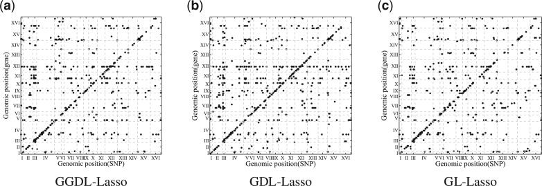
The top-1000 significant associations given by GGDL, GDL and G-Lasso are shown in Figure 6. We can see that GGDL and GDL have stronger cis-regulatory signals than G-Lasso does. In total, these methods each detected ∼6000 associations according to non-zero W values. We estimate FDR using 50 permutations as proposed in (Yang et al., 2013). With FDR ≤ 0.01, GGDL obtains ∼4500 significant associations. The plots of all identified significant associations for different methods are given in the Supplementary Material.
Fig. 6.
The top-1000 significant associations identified by different methods. In each plot, the x-axis represents SNPs and y-axis represents genes. Both SNPs and genes are arranged by their locations in the genome
5.2.2 Refinement of the prior networks
To investigate to what extend GGDL is able to refine the prior networks and study the effect of different parameter settings on κ, we intentionally change 75% elements in the original prior PPI network and genetic-interaction network to random noises. We feed the new networks to GGDL and evaluate the refined networks. The results are shown in Figure 7. We can see that for both PPI and genetic-interaction networks, many elements are recovered by GGDL. This demonstrates the effectiveness of GGDL. Moreover, when the number of SNP (gene) pairs (κ) examined for updating reaches 100 000, both PPI and genetic-iteration networks are well refined.
Fig. 7.
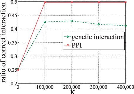
Ratio of correct interactions refined when varying κ. The initial input networks only contain 25% correct interactions
5.2.3 Hotspots analysis
In this section, we study whether GGDL can help detect more biologically relevant associations than the alternatives. Specifically, we examine the hotspots which affect >10 gene traits (Lee and Xing, 2012). The top-15 hotspots detected by GGDL are listed in Table 3. The top-15 hotspots detected by other methods are included in the Supplementary Material. From Table 3, we observe that for all hotspots, the associated genes are enriched with at least one GO category. Note that GGDL and GDL detect one hotspot (12), which cannot be detected by G-Lasso. They also detect one hotspot (6), which can not be detected by SIOL. The number of hotspots that are significant enriched is listed in Table 4. From the table, we can see that GGDL slightly outperforms GDL since it incorporates the location of SNPs and gene-pathway information.
Table 3.
Summary of the top-15 hotspots detected by GGDL
| ID | Sizea | Locib | GOc | Hitsd | GDL (all)e | GDL (hits)f | G-Lasso(all)g | G-Lasso(hits)h | SIOL(all)i | SIOL(hits)j | LORS(all)k | LORS(hits)l |
|---|---|---|---|---|---|---|---|---|---|---|---|---|
| 1 | 31 | XII:1056097 | (1)*** | 7 | 31 | 7 | 32 | 7 | 8 | 6 | 31 | 7 |
| 2 | 28 | III:81832..92391 | (2)** | 5 | 29 | 5 | 28 | 5 | 58 | 5 | 22 | 4 |
| 3 | 28 | XII:1056103 | (1)*** | 7 | 29 | 6 | 28 | 6 | 1 | 1 | 2 | 0 |
| 4 | 27 | III:79091 | (2)*** | 6 | 29 | 6 | 28 | 6 | 28 | 7 | 10 | 2 |
| 5 | 27 | III:175799..177850 | (3)* | 3 | 26 | 3 | 23 | 3 | 9 | 2 | 18 | 4 |
| 6 | 27 | XII:1059925..1059930 | (1)*** | 7 | 27 | 7 | 27 | 7 | 0 | 0 | 5 | 1 |
| 7 | 25 | III:105042 | (2)*** | 6 | 23 | 6 | 25 | 6 | 5 | 3 | 19 | 4 |
| 8 | 23 | III:201166..201167 | (3)*** | 3 | 23 | 3 | 22 | 3 | 13 | 2 | 23 | 3 |
| 9 | 22 | XII:1054278..1054302 | (1)*** | 7 | 26 | 7 | 24 | 7 | 24 | 5 | 12 | 4 |
| 10 | 21 | III:100213 | (2)** | 5 | 23 | 5 | 23 | 5 | 5 | 3 | 5 | 1 |
| 11 | 20 | III:209932 | (3)* | 3 | 21 | 3 | 19 | 3 | 16 | 4 | 15 | 4 |
| 12 | 20 | XII:659357..662627 | (4)* | 4 | 19 | 4 | 3 | 0 | 37 | 9 | 36 | 6 |
| 13 | 19 | III:210748..210748 | (5)* | 4 | 24 | 4 | 18 | 4 | 2 | 3 | 11 | 4 |
| 14 | 19 | VIII:111679..111680 | (6)* | 3 | 20 | 3 | 19 | 3 | 3 | 3 | 12 | 2 |
| 15 | 19 | VIII:111682..111690 | (7)** | 5 | 21 | 5 | 20 | 5 | 57 | 6 | 22 | 3 |
| Total hits | 75 | 74 | 70 | 59 | 49 | |||||||
aNumber of genes associated with the hotspot bThe chromosome position of the hotspot. cThe most significant GO category enriched with the associated gene set. The enrichment test was performed using DAVID (Huang et al., 2009). The gene function is defined by GO category. The involved GO categories are: (i) telomere maintenance via recombination; (ii) branched chain family amino acid biosynthetic process; (iii). regulation of mating-type specific transcription, DNA-dependent; (iv) sterol biosynthetic process; (v) pheromone-dependent signal transduction involved in conjugation with cellular fusion; (vi) cytogamy; (vii) response to pheromone. dNumber of genes that have enriched GO categories. e,g,I,kNumber of associated genes that can also be identified using GDL, G-Lasso, SIOL and LORS, respectively. f,h,j,lNumber of genes that have enriched GO categories and can also be identified by GDL, G-Lasso, SIOL and LORS, respectively. Among these hotspots, hotspot (12) in bold cannot be detected by G-Lasso. Hotspot (6) in italic cannot be detected by SIOL. Hotspot (3) in teletype cannot be detected by LORS. Adjusted P-values using permutation tests. *10–2∼10−3, **10−3∼10−5, ***10−5∼10−10.
Table 4.
Hotspots detected by different methods
| GGDL | GDL | G-Lasso | SIOL | LORS | |
|---|---|---|---|---|---|
| Number of hotspots significantly enriched (top 15 hotposts) | 15 | 14 | 13 | 10 | 9 |
| Number of total reported hotspots (size > 10) | 65 | 82 | 96 | 89 | 64 |
| Number of hotspots significantly enriched | 45 | 56 | 61 | 53 | 41 |
| Ratio of significantly enriched hotspots (%) | 70 | 68 | 64 | 60 | 56 |
6 DISCUSSION
As a promising tool for dissecting the genetic basis of common diseases, eQTL study has attracted increasing research interest. The traditional eQTL methods focus on testing the associations between individual SNPs and gene expression traits. A major drawback of this approach is that it cannot model the joint effect of a set of SNPs on a set of genes, which may correspond to biological pathways.
Recent advancement in high-throughput biology has made a variety of biological interaction networks available. Effectively integrating such prior knowledge is essential for accurate and robust eQTL mapping. However, the prior networks are often noisy and incomplete. In this article, we propose novel graph-regularized-regression models to take into account the prior networks of SNPs and genes simultaneously. Exploiting the duality between the learned coefficients and incomplete prior networks enables more robust model. We also generalize our model to integrate other types of information, such as SNP locations and gene pathways. The experimental results on both simulated and real eQTL datasets demonstrate that our models outperform alternative methods. In particular, the proposed dual refinement regularization can significantly improve the performance of eQTL mapping.
Funding: National Institutes of Health (grants R01HG006703 and P50 GM076468-08); NSF IIS-1313606; NSF IIS-1162374 and IIS-1218036.
Conflict of Interest: none declared.
REFERENCES
- Biganzoli EM, et al. Artificial neural network for the joint modelling of discrete cause-specific hazards. Artif. Intell. Med. 2006;37:119–130. doi: 10.1016/j.artmed.2006.01.004. [DOI] [PubMed] [Google Scholar]
- Bochner BR. New technologies to assess genotype henotype relationships. Nat. Rev. Genet. 2003;4:309–314. doi: 10.1038/nrg1046. [DOI] [PubMed] [Google Scholar]
- Boyd S, Vandenberghe L. Convex Optimization. Cambridge: Cambridge University Press; 2004. [Google Scholar]
- Brem RB, et al. Genetic interactions between polymorphisms that affect gene expression in yeast. Nature. 2005;436:701–703. doi: 10.1038/nature03865. [DOI] [PMC free article] [PubMed] [Google Scholar]
- Brem YG, et al. Trans-acting regulatory variation in Saccharomyces cerevisiae and the role of transcription factors. Nat. Genet. 2003;35:57–64. doi: 10.1038/ng1222. [DOI] [PubMed] [Google Scholar]
- Charles Boone HB, Andrews BJ. Exploring genetic interactions and networks with yeast. Nat. Rev. Genet. 2007;8:437C449. doi: 10.1038/nrg2085. [DOI] [PubMed] [Google Scholar]
- Chen X, et al. 2012. A two-graph guided multi-task lasso approach for eqtl mapping. In AISTATS, pp. 208–217. La Palma, Canary Islands. [Google Scholar]
- Chung FRK. CBMS: Conference Board of the Mathematical Sciences, Regional Conference Series. Vol. 92. Washington, DC: Published for the Conference Board of the Mathematical Sciences; 1997. Spectral graph theory (reprinted with corrections) [Google Scholar]
- Ding C, et al. 2006. Orthogonal nonnegative matrix t-factorizations for clustering. In KDD, ACM, New York, pp. 126–135. [Google Scholar]
- Ding CHQ, et al. Convex and semi-nonnegative matrix factorizations. IEEE Trans. Pattern Anal. Mach. Intell. 2010;32:45–55. doi: 10.1109/TPAMI.2008.277. [DOI] [PubMed] [Google Scholar]
- Huang DAW, et al. Systematic and integrative analysis of large gene lists using DAVID bioinformatics resources. Nat. Protoc. 2009;4:44–57. doi: 10.1038/nprot.2008.211. [DOI] [PubMed] [Google Scholar]
- Jenatton R, et al. Structured variable selection with sparsity-inducing norms. JMLR. 2011;12:2777–2824. [Google Scholar]
- Kim S, Xing EP. Statistical estimation of correlated genome associations to a quantitative trait network. PLoS Genet. 2009;5:e1000587. doi: 10.1371/journal.pgen.1000587. [DOI] [PMC free article] [PubMed] [Google Scholar]
- Kim S, Xing EP. Tree-guided group lasso for multi-response regression with structured sparsity, with applications to eQTL mapping. Ann. Appl. Stat. 2012;6:1095–1117. [Google Scholar]
- Lander ES. Initial impact of the sequencing of the human genome. Nature. 2011;470:187–197. doi: 10.1038/nature09792. [DOI] [PubMed] [Google Scholar]
- Lee DD, Seung HS. Algorithms for non-negative matrix factorization. NIPS. 2000;13:556–562. [Google Scholar]
- Lee S, Xing EP. Leveraging input and output structures for joint mapping of epistatic and marginal eQTLs. Bioinformatics. 2012;28:i137–i146. doi: 10.1093/bioinformatics/bts227. [DOI] [PMC free article] [PubMed] [Google Scholar]
- Lee S, et al. Adaptive multi-task lasso: with application to eQTL detection. NIPS. 2010 pp. 1306–1314, Vancouver, British Columbia, Canada. [Google Scholar]
- Li C, Li H. Network-constrained regularization and variable selection for analysis of genomic data. Bioinformatics. 2008;24:1175–1182. doi: 10.1093/bioinformatics/btn081. [DOI] [PubMed] [Google Scholar]
- Listgarten J, et al. Correction for hidden confounders in the genetic analysis of gene expression. Proc. Natl Acad. Sci. USA. 2010;107:16465–16470. doi: 10.1073/pnas.1002425107. [DOI] [PMC free article] [PubMed] [Google Scholar]
- Mazumder R, et al. Spectral regularization algorithms for learning large incomplete matrices. JMLR. 2010;11:2287–2322. [PMC free article] [PubMed] [Google Scholar]
- Michaelson J, et al. Detection and interpretation of expression quantitative trait loci (eQTL) Methods. 2009;48:265–276. doi: 10.1016/j.ymeth.2009.03.004. [DOI] [PubMed] [Google Scholar]
- Musani SK, et al. Detection of gene x gene interactions in genome-wide association studies of human population data. Hum. Hered. 2007;63:67–84. doi: 10.1159/000099179. [DOI] [PubMed] [Google Scholar]
- Obozinski G, Taskar B. Multi-task feature selection. 2006 Technical report 709. Statistics Department, University of California, Berkeley. [Google Scholar]
- Pujana MA, et al. Network modeling links breast cancer susceptibility and centrosome dysfunction. Nat. Genet. 2007;39:1338–1349. doi: 10.1038/ng.2007.2. [DOI] [PubMed] [Google Scholar]
- Tibshirani R. Regression shrinkage and selection via the lasso. J. Royal. Statist. Soc. B. 1996;58:267–288. [Google Scholar]
- von Mering C, et al. Comparative assessment of large-scale data sets of protein-protein interactions. Nature. 2002;417:399–403. doi: 10.1038/nature750. [DOI] [PubMed] [Google Scholar]
- Yang C, et al. Accounting for non-genetic factors by low-rank representation and sparse regression for eQTL mapping. Bioinformatics. 2013;29:1026–1034. doi: 10.1093/bioinformatics/btt075. [DOI] [PMC free article] [PubMed] [Google Scholar]


