ExSPAnder: a universal repeat resolver for DNA fragment assembly

Abstract

Next-generation sequencing (NGS) technologies have raised a challenging de novo genome assembly problem that is further amplified in recently emerged single-cell sequencing projects. While various NGS assemblers can use information from several libraries of read-pairs, most of them were originally developed for a single library and do not fully benefit from multiple libraries. Moreover, most assemblers assume uniform read coverage, condition that does not hold for single-cell projects where utilization of read-pairs is even more challenging. We have developed an exSPAnder algorithm that accurately resolves repeats in the case of both single and multiple libraries of read-pairs in both standard and single-cell assembly projects.

Availability and implementation: http://bioinf.spbau.ru/en/spades

Contact: ap@bioinf.spbau.ru

1 INTRODUCTION

Most of existing next-generation sequencing (NGS) platforms generate read-pairs—pairs of reads (called mates) that are sequenced from different ends of a genomic fragment with approximately known length (called the insert size). Because the insert size usually exceeds the length of a single read, read-pairs may match up unique regions surrounding repeats that are longer than the read length. A combination of several libraries of read-pairs with different insert sizes is often used to produce high-quality assemblies (Butler et al. 2008; Bresler et al., 2012). Paired-end libraries usually have insert size <1 kb and are used for resolving relatively short repeats. Jumping libraries are characterized by an average insert size of anywhere from 1 to 20 kb and are helpful in resolving longer repeats and contig scaffolding (inferring the order of contigs in the genome). However, because of a high insert size variation, information from jumping libraries is rather difficult to use for the purpose of assembly.

The problem of using multiple read-pair libraries was previously addressed by ALLPATHS-LG (Gnerre et al., 2011), Ray (Boisvert et al., 2010), Velvet (Zerbino and Birney, 2008) and some other assemblers. However, these tools are designed for standard (mutlicell) assemblies and do not perform well on single-cell datasets. On the other hand, the single-cell assemblers ESC (Chitsaz et al., 2011), IDBA-UD (Peng et al., 2012) and SPAdes (Bankevich et al., 2012) are designed for a single read-pair library. In addition, the recently proposed Paired de Bruijn Graph algorithms for repeat resolution (Medvedev et al., 2011; Pham et al., 2013; Vyahhi et al., 2012) also focus on a single library and it remains unclear how to extend them to multiple libraries.

We present exSPAnder algorithm that works with both single and multiple libraries in standard and single-cell assembly projects. exSPAnder uses a simple path extension approach for repeat resolution that was originally proposed in the Ray assembler [and later used in Telescoper (Bresler et al., 2012)] and combines it with some ideas from the Rectangle Graph approach (Bankevich et al., 2012; Vyahhi et al., 2012). Given a set of paths in the assembly graph (Bankevich et al., 2012) (i.e. simplified de Bruijn graph (Compeau et al., 2011; Pevzner et al., 2001) of k-mers in reads after removal of bulges, tips and chimeric edges), exSPAnder attempts to extend each path with the goal to generate longer paths. For a path P ending in a vertex v, we consider all edges starting at v (referred to as extension edges) and compute Score_P(e) for each extension edge. To compute Score_P(e) we analyze all reads that map to path P and whose mates map to e. Thus, Score_P(e) reflects our confidence that an extension of the path P by the edge e is correct. We note that to properly map read-pairs and calculate Score_P(e), the total length of path P and edge e should be longer than the insert size.

In addition to function Score_P(e), exSPAnder uses a decision rule Extend(P) that either chooses one of the extension edges to extend the path P or makes the decision to stop growing this path beyond the ending vertex of P. The procedure is iterated over all the paths until no path can be further extended. To initiate this algorithm one can start with a set of single-edge paths formed by all sufficiently long edges in the assembly graph. The resulting paths are output as contigs after removing the paths that are contained within other paths as well as removing non-informative overlaps (i.e. suffixes of paths that represent prefixes of other paths).

This simple approach is merely a framework and, depending on the specifics of the scoring function and the decision rule, it can be either efficient (like in the Ray assembler) or disastrous. The authors of Telescoper made an attempt to improve on Ray’s scoring function and to substantiate it with rigorous statistical analysis. However, scoring functions in both Ray and Telescoper are not universal, e.g. they assume the uniform genome coverage by reads, condition that does not hold for single-cell data.

We demonstrate that exSPAnder works well on single-cell datasets with multiple libraries. We also show that exSPAnder [implemented as a part of SPAdes (Bankevich et al., 2012)] improves on existing assemblers on standard bacterial datasets and outperforms such popular assemblers as ABySS (Simpson et al., 2009), Ray (Boisvert et al., 2010), SOAPdenovo (Li et al., 2010) and Velvet (Zerbino and Birney, 2008). ALLPATHS-LG (Gnerre et al., 2011) is an excellent assembler whose applications, however, are limited to specially constructed read-pair libraries. On such libraries exSPAnder and ALLPATHS-LG generate comparable results (exSPAnder generates longer contigs but ALLPATHS-LG generates longer scaffolds).

2 ANALYSIS OF READ-PAIR LIBRARIES

As we mentioned in the introduction, jumping libraries present additional challenges for genome assembly owing to their high variations in the insert size. Additionally, jumping libraries have high rate of chimeric read-pairs—read-pairs that either have abnormal insert size or incorrect orientation. Chimeric read-pairs further complicate utilization of such libraries while resolving repeats.

Below we present analysis of the insert size distributions for the following data: Brachybacterium faecium isolate dataset (read length 150 bp) and Staphylococcus aureus single-cell dataset (read length 101 bp). Both datasets contain one paired-end and one jumping library. To analyze read-pair libraries we aligned reads to the B.faecium and S.aureus reference genomes using Bowtie 2 (Langmead and Salzberg, 2012) and computed the chimeric read-pair rates and insert size distributions.

As Figure 1 and Table 1 demonstrate, both isolate and single-cell paired-end libraries have small variations of the insert size. In contrast, the jumping library from the B.faecium dataset has a much higher variation in the insert size and higher rate of chimeric read-pairs (Table 1). At the same time, in addition to the large insert size variations, S.aureus jumping library contains only 22% of all read-pairs aligned with the proper reverse–forward orientation. Thirty-six percent of all read-pairs have incorrect forward–reverse orientation (correspond to the left peak in Fig. 1d) and 14% are classified as chimeric read-pairs of other types. Forward–reverse read-pairs in jumping libraries represent an artifact of the sample preparation and are common for datasets of different types.

Fig. 1.

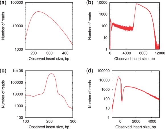
Plots of the insert size distributions for B.faecium isolate (a) paired-end and (b) jumping library, and S.aureus single-cell dataset with (c) paired-end and (d) jumping library. The distributions were computed by mapping reads to the B.faecium str. DSM4810 (Lapidus et al., 2009) and S. aureus str. USA300 substr. FPR3757 (Diep et al., 2006) reference genomes, respectively. All plots are in the logarithmic scale

Table 1.

Information on the B.faecium isolate dataset and the S.aureus single-cell dataset

Dataset	B.faecium		S.aureus
Library	Paired-end	Jumping	Paired-end	Jumping
Number of reads	13 M	41 M	38 M	41 M
Average coverage	400×	1100×	1050×	1050×
Coverage span	210–570×	0–3000×	0–3500×	0–3500×
Insert size	270 bp	7.5 kb	210 bp	1.8 kb
Insert span	150–400 bp	6–10 kb	180–230 bp	0.5–4 kb
Chimeric read-pairs (%)	1	9	3	50
Unaligned read-pairs (%)	16	10	6	28

Note: Insert span is the shortest insert size interval that contains at least 95% of properly aligned read-pairs. Unaligned reads refer to the percentage of read-pairs that have at least one read unaligned. Chimeric read-pairs refer to the percentage of chimeric read-pairs among all read-pairs. All statistics was obtained using Bowtie 2 (Langmead and Salzberg, 2012). Coverage span is the smallest coverage interval that includes a least 95% of all genomic positions

Despite the fact that various artifacts of jumping libraries make it difficult to incorporate them into existing assembly tools, exSPAnder uses jumping libraries to generate high-quality assemblies.

3 EXSPANDER ALGORITHM

exSPAnder uses an assembly graph constructed by SPAdes (Bankevich et al., 2012) and a set of read-pair libraries. For each library, we map read-pairs to the long edges of the assembly graph and estimate the average insert size along with its confidence interval—a shortest insert size interval that contains at least 80% of properly aligned read-pairs. These estimates are used as parameters of the scoring function and the decision rule.

3.1 The decision rule

3.1.1 Single library

Given a path P, we define a winner as an edge e with the maximal score Score_P(e) among all extension edges for P. Similarly, a contender is defined as an extension edge with the second best score. The winner edge is called the strong winner if (i) Score_P(winner) >Θ and (ii) Score_P(winner) > C · Score_P(contender), where Θ and C are parameters of the algorithm, which are discussed below. If the path P has a single extension edge (which is obviously the winner), only the first condition is used. The decision rule is defined as follows:

$$Extend(P)=\{\begin{array}{ll}e,\hfill & \text{if edge}e\text{is the strong winner for path}P\hfill \\ \varnothing ,\hfill & \text{if there is no strong winner for path}P\hfill \end{array}$$

3.1.2 Multiple libraries

The decision rule described above can be generalized for several read-pair libraries. Consider M read-pair libraries, which are sorted in the order of increasing insert sizes and the associated decision rules Extend_i(P) for 1 ≤ i ≤ M. We process the libraries in this order because our analysis revealed that the smaller is the insert size of a library (and its variation), the more reliable is the decision rule for this individual library. We thus select the library with the smallest index i that has the strong winner and define the decision rule for multiple libraries Extend(P) as simply Extend_i(P). If neither library has a strong winner, we define $Extend(P)=\varnothing$.

3.2 The scoring function

3.2.1 The support function

We first consider an idealized case when the genome defines a genomic path in the assembly graph. We say that an edge e′ follows edge e at a distance D if the distance between starts of these edges in the genomic path is D. We define a boolean function Support_D(e,e′) that reflects our confidence that edge e′ follows edge e in the genome at distance D. Below we describe how to calculate Support_D(e,e′).

Let I and [I_min,I_max] be the mean and the confidence interval of the insert size for a read-pair library formed by reads of length ReadLength. Consider consecutive edges e and e′ in the assembly graph and a read-pair (r,r′) such that read r maps to e at position x₀ and read r′ maps to e′ in position y₀ (Fig. 2a). We say that the read-pair (r,r′) connects edges e and e′. Figure 2b shows a rectangle formed by the edges e and e′ [further simply referred to as rectangle (e,e′)] with the read-pair (r,r′) represented as a point (x₀,y₀) within the rectangle. If edges e and e′ represent consecutive regions in the genome, then the genomic distance from the start of read r to the start of read r′ equals to $Length(e)-x_0+y_0$, where Length(e) stands for the length of edge e. Therefore, in the case of an ‘ideal read-pair’ (r,r′) (e.g. a read-pair with the exact insert size I), $y_0=x_0-d$, where $d=Length(e)-I+ReadLength$. Thus all ‘ideal read-pairs’ mapping to edges e and e′ form a set of integer points on the 45° line y = x– d within the rectangle (Fig. 2c). Because the read-pairs from the real sequencing data have variations in the insert size, their corresponding points are typically scattered in the strip between the 45° lines y = x – d_min and y = x – d_max, where

$$\begin{array}{l}{d}_{min}=Length(e)-I_{min}+ReadLength,\\ d_{max}=Length(e)-I_{max}+ReadLength.\end{array}$$

This strip in the rectangle is further referred to as the confidence strip (Fig. 2d).

Fig. 2.

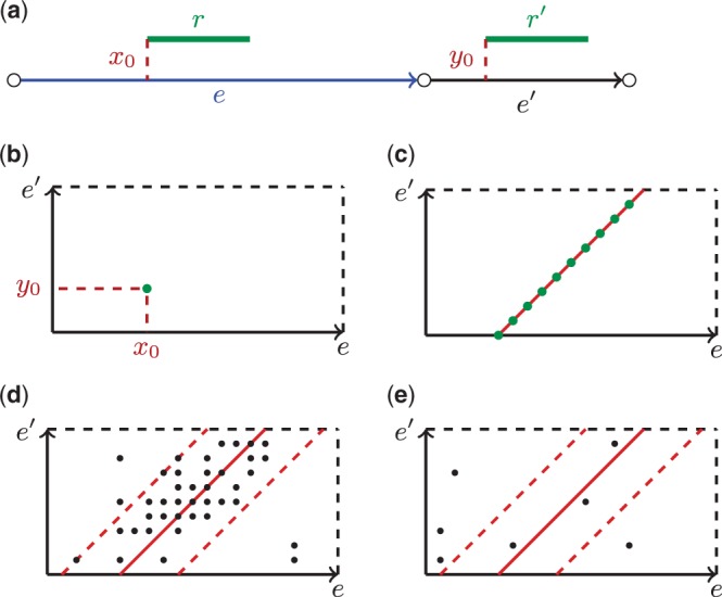
(a) Reads r and r′ form a read-pair mapping to consecutive edges e and e′ in the assembly graph at positions x₀ and y₀, respectively. (b) Representation of a read-pair (r,r′) as a point in a rectangle (e,e′). (c) ‘Ideal read-pairs’ with the exact insert size I connecting edges e and e′ form a 45° line within a rectangle. (d) Read-pairs from the real sequencing data with variations in the insert size represented as points within a rectangle. Most points are located within the confidence strip providing the evidence that edges e and e′ are supported by the read-pairs and are genome-consecutive. (e) A rectangle formed by a pair of edges that has few points falling into the confidence strip revealing that e and e′ are not genome-consecutive edges

Let F(x) be the empirical distribution of the insert size and S be a set of all integer points within the confidence strip in the rectangle (e,e′). We define the expected number of read-pairs within the confidence strip (under the assumption of the uniform coverage) as

$$Expected(e,e\prime )={\displaystyle \sum _{(x,y)\in S}F}(I(x,y)),$$

where $I(x,y)=Length(e)-x+y+ReadLength$ represents the insert size of a read-pair that corresponds to the point (x, y). We also define Points(e,e′) as the total number of read-pairs (from the real dataset) that correspond to the points within the confidence strip. The notion of density is defined as

$$Density(e,e\prime )=\frac{Points(e,e\prime )}{Expected(e,e\prime )}.$$

We set Density(e,e′) = 0, if Expected(e,e′) = 0. The points outside the confidence strip may represent read-pairs with somewhat larger deviations from the mean insert sizes or chimeric read-pairs. Our analysis revealed that being conservative (e.g. limiting analysis to the confidence strip) allows one to avoid most of the assembly errors caused by chimeric read-pairs, particularly in single-cell projects.

We distinguish between notions of genome-consecutive and graph-consecutive edges and emphasize that graph-consecutive edges are not necessarily genome-consecutive. The decision about which graph-consecutive edges are genome-consecutive is an important part of any assembler. Figure 2d and e illustrate how rectangles help us to make such decisions: both rectangles correspond to graph-consecutive edges, but only rectangle in Figure 2d is formed by the pair of genome-consecutive edges.

The described notions of Expected(e,e′), Points(e,e′) and Density(e,e′) (defined for the case when edges e and e′ are genome-consecutive) can be generalized for the case when e and e′ are not consecutive genomic edges under the assumption that genomic distance between them is D. In this case the confidence strip [further referred to as Strip_D(e,e′)] is bounded by the lines y = x – d_min and y = x – d_max, where

$$\begin{array}{l}{d}_{min}=D-I_{min}+ReadLength,\\ d_{max}=D-I_{max}+ReadLength.\end{array}$$

Points_D(e,e′) similarly represents the number of points within strip Strip_D(e,e′). Expected_D(e,e′) and Density_D(e,e′) are defined using the same formulas and the corresponding confidence strip. Clearly, for two genome-consecutive edges Expected(e,e′) = Expected_L(e,e′) and Density(e,e′) = Density_L(e,e′), where L = Length(e).

The support function reflects whether the number of read-pairs connecting edges e and e′ supports the conjecture that e′ follows e in the genome at distance D:

$$Suppor{t}_D(e,e\prime )=\{\begin{array}{ll}1,\hfill & Densit{y}_D(e,e\prime )>\Psi \hfill \\ 0,\hfill & \text{otherwise}\hfill \end{array}$$

where Ψ is a parameter of the algorithm, which is automatically computed for each read-pair library based on the chimeric read-pair rate (see below). For the standard isolate datasets this parameter corresponds to the coverage cutoff for read-pairs. For single-cell datasets this parameter is usually set to be very low to retain the regions with low coverage, which are typical for single-cell projects. If Support_D(e,e′) = 1, we say that the rectangle (e,e′) is supported by the read-pairs.

3.2.2 The naive scoring function

To explain the intuition behind exSPAnder, we first introduce the naive scoring function. We further modify the naive scoring function to arrive to the advanced scoring function used in the real exSPAnder implementation.

A path P = (p₁, … ,p_m) and its extension edge e can be represented as a composite rectangle formed by m simple rectangles (p_j,e) containing points that correspond to read-pairs connecting edges of P and e. Figure 3b shows an example of a composite rectangle, which is formed by a path (p₁, p₂, p₃) and its extension edge e₁ and consists of three simple rectangles. The notion of the confidence strip remains (it now consists of up to m substrips within simple rectangles), except that it is bounded by the lines y = x – d_min and y = x – d_max, where

$$\begin{array}{l}{d}_{min}=Length(P)-I_{min}+ReadLength,\\ d_{max}=Length(P)-I_{max}+ReadLength.\end{array}$$

For an edge p_j from the path P we define the expected number of points in the confidence substrip within the simple rectangle (p_j,e) as $Expecte{d}_{D_j}(p_j,e)$, where D_j is the distance between start of p_j and start of e according to the path P (i.e. $D_j={\sum }_{i=j}^{m}Length(p_i)$). We consider rectangles $(p_j,e),j=start,\dots ,end$ such that $Expecte{d}_{D_j}(p_j,e)>0$ and introduce the function Score_P(e) as the fraction of the total number of expected read-pairs in these rectangles with $Suppor{t}_{D_j}(p_j,e)=1$:

$$Scor{e}_P(e)=\frac{{\displaystyle \sum _{j=start}^{end}S}uppor{t}_{D_j}(p_j,e)·Expecte{d}_{D_j}(p_j,e)}{{\displaystyle \sum _{j=start}^{end}E}xpecte{d}_{D_j}(p_j,e)}.$$

We set Score_P(e) = 0 if all simple rectangle have zero expected read-pairs.

Fig. 3.

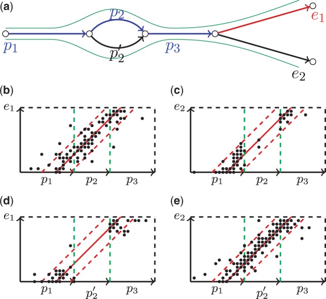
(a) An example of an assembly graph with the genomic paths (p₁, p₂, p₃, e₁) and $(p_1,p{\prime }_2,p_3,e_2)$. (b, e) The composite rectangles for correct genomic extension of each path: in these cases the points are evenly distributed within the confidence strip and the resulting score is equal to 1. (c, d) The composite rectangles that correspond to incorrect extensions edges of these two paths. In each of these cases, at least one simple rectangle contains few points within the confidence strip

Figure 3a shows paths P = (p₁, p₂, p₃) and P′ = (p₁,p′₂, p₃) and its extension edges e₁,e₂. Let (p₁, p₂, p₃, e₁) and (p₁,p′₂,p₃, e₂) be the true (but unknown) genomic paths. Figure 3b shows the composite rectangle for path P and its correct extension e₁, in which points within the confidence strip are rather evenly distributed resulting in Score_P(e₁) = 1. Figure 3c shows the composite rectangle for path P = (p₁, p₂, p₃) and its incorrect extension edge e₂. Because (p₁, p′₂, p₃, e₂) is a genomic path, density of the points in the sectors of the confidence strip corresponding to edges p₁ and p₃ is high. However, edge p₂ of the path P does not support extension edge e₂ because there are few points in the rectangle (p₂, e₂). Additionally, Figure 3d and e shows composite rectangles for all possible extension edges for path P′ = (p₁, p′₂, p₃).

Because the defined scoring function does not linearly depend on read coverage, it is well suitable for both single-cell and standard sequencing projects. At the same time, considering only read-pairs with insert size in [I_min,I_max] (which correspond to points within the confidence strip) allows one to filter out most of the chimeric read-pairs (common for single-cell datasets) and to minimize their influence on the scoring function.

3.2.3 The advanced scoring function

The naive scoring function Score_P(e) described above works well in many cases but may be too conservative when the path P contains repetitive edges (edges that are visited more than once by the genomic traversal). Figure 4 illustrates the case when the path P has a repetitive edge and motivates the need for further improvements in the scoring function.

Fig. 4.

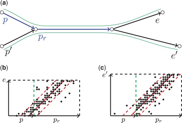
Scoring a path that contains repetitive edges. (a) An example of the assembly graph with a repetitive edge p_r. (b) A composite rectangle for the correct extension e of path (p,p_r). (c) A composite rectangle for the incorrect extension e′ of the path (p,p_r)

Figure 4a shows an assembly graph with four unique edges (p, p′, e and e′) and a single repetitive edge p_r with multiplicity 2. We assume that paths (p,p_r,e) and (p′,p_r,e′) are genomic and paths (p,p_r,e′) and (p′,p_r,e) are non-genomic. Our goal is to design an algorithm that correctly extends genomic paths (p,p_r) and (p′,p_r) into longer genomic paths (p,p_r,e) and (p′,p_r,e′), respectively.

Consider a path P = (p,p_r) and composite rectangles (P,e) and (P,e′) (Fig. 4b and c). As Figure 4 illustrates, Score_P(e) is similar to Score_P(e′), implying that there is no strong winner for path P and preventing us from extending the path P by edge e. However, because the repetitive edge p_r supports both extension edges e and e′, it does not provide any valuable information about the correct extension of the path P. Therefore, to make a decision about extending the path P by an extension edge e, we should have excluded p_r from the consideration as a repetitive edge. Because we do not know in advance which edges of the assembly graph correspond to repeats in the genome, we classify p_r as repetitive because it supports both extension edges e and e′.

Below we present the exSPAnder algorithm that allows us to exclude repetitive edges from contributing to scoring. An extension edge e of path P is called an active edge if $C·Scor{e}_P(e)\ge Scor{e}_P(winner)$. At the first step of the algorithm we score all extension edges and form a set of active edges $\mathcal{A}$. An edge p_j in path P is classified as repetitive if it supports all active edges, i.e. $Suppor{t}_{D_j}(p_j,e_i)=1$ for all $e_i\in \mathcal{A}$. At the second step we mark all repetitive edges $p_j\in P$ and recalculate scores of all edges in $\mathcal{A}$ ignoring these repetitive edges. We then update $\mathcal{A}$ by removing all non-active edges and iterate the process. The process continues until yet another iteration does not change the set of active edges $\mathcal{A}$. If $\mathcal{A}=\left\{e\right\}$ and Score_P(e) >Θ (which means that e satisfies both conditions in the decision rule) the extension edge e is considered to be a strong winner and added to the path P. Otherwise, we stop extending path P.

We further demonstrate the work of the exSPAnder algorithm using a simple assembly graph shown in Figure 5. The paths $(p_1,p_2,p_3,e_1),(p{\prime }_1,p_2,p_3,e_2)$ and $(p{\prime }_2,p_3,e_3)$ are genomic paths, which means that edges p₂ and p₃ are repetitive and have multiplicities 2 and 3, respectively.

Fig. 5.

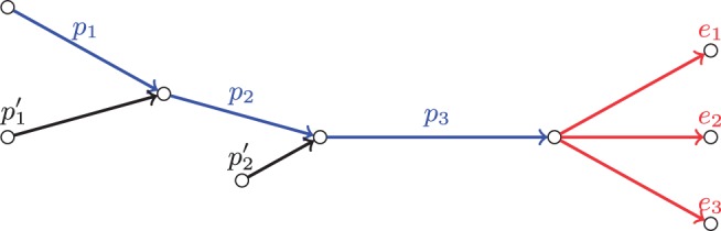
An example of the assembly graph with repetitive edges p₂ and p₃

Let P = (p₁, p₂, p₃) be a path we aim to extend. We first calculate scores of all extension edges using the composite rectangles (Fig. 6a–c) and form a set of active edges $\mathcal{A}=\{e_1,e_2,e_3\}$ based on their scores (marked red in Fig. 6d). Because $Suppor{t}_{D_3}(p_3,e_i)=1$ for i = 1, 2, 3, edge p₃ is classified as repetitive and is removed from further consideration (Fig. 6e). We now recalculate scores for the extension edges in $\mathcal{A}$ ignoring repetitive edge p₃ (Fig. 6f–h) and remove non-active edge e₃ from $\mathcal{A}$ (Fig. 6i). Using the updated set $\mathcal{A}=\{e_1,e_2\}$ we again proceed to the repeat detection step and mark edge p₂ as repetitive because $Suppor{t}_{D_2}(p_2,e_i)=1$ for i = 1, 2 (Fig. 6j). Finally, we once again recalculate scores of the extension edges in $\mathcal{A}$ (Fig. 6k–m) and remove e₂ as non-active (Fig. 6n). The extension edge e₁ remains the only active edge in and is used to extend path P.

Fig. 6.

A step-by-step example of the exSPAnder algorithm. (a–c) Forming a set of active edges {e₁, e₂, e₃} (marked red) for the path P = (p₁, p₂, p₃) using the corresponding composite rectangles. (d, e) Classifying of edge p₃ as repetitive and removing it from further consideration (marking gray). Edges that are not classified as repetitive are colored in blue. (f–h) Recalculating scores of the extension edges and updating the set of active edges. (i, j) Removing repetitive edge p₂. (k–m) Recalculating scores for the remaining active edges {e₁, e₂} and removing e₂ as non-active. (n) Selecting the only active edge e₁ as an extension for the path P

Extensive tests of the advanced scoring function revealed that it works well across diverse datasets including single-cell jumping libraries with high variations in the insert size, extremely non-uniform coverage and large number of chimeric reads and chimeric read-pairs (see Section 4).

3.3 Scaffolding

After all paths are constructed, we consider all pairs of paths that form composite rectangles with non-zero number of points (Fig. 7). For each such pair of paths P and P′ we can check whether points in the corresponding composite rectangle are scattered around a certain 45° line using SPAdes distance estimation procedure (Nurk et al., 2013). When SPAdes provides the estimated distance D between P and P′, we use exSPAnder to verify the conjecture that P′ follows P at distance D. If this conjecture is supported and does not contradict to any other conjectures about these paths, we extend the path P by P′ (the scaffolding step). We estimate the gap length between the paths as $D-Length(P)$ and insert the appropriate number of ‘N’ symbols (unspecified nucleotide) between end of P and start of P′. If paths P and P′ overlap, we construct their overlap alignment to correct distance D.

Fig. 7.

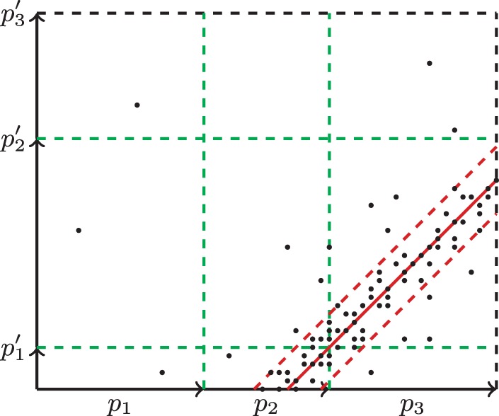
An example of a composite rectangle formed by paths (p₁, p₂, p₃) and $(p{\prime }_1,p{\prime }_2,p{\prime }_3)$

3.4 Choice of the parameters

3.4.1 The scoring function

We select the parameter Ψ as a threshold for the density of the read-pairs within the confidence strip. We therefore assume that rectangles with the density below Ψ contain mostly chimeric read-pairs and should be ignored while calculating the score of an extension edge. To select Ψ for a particular read-pair library, we estimate the distribution of the densities for rectangles that contain only chimeric read-pairs (false rectangles) and for rectangles that contain only non-chimeric read-pairs (true rectangles).

To partition all read-pairs into chimeric and non-chimeric, one needs the complete genome that is unavailable. To get around this, we identify a subset of chimeric reads using the long edges in the assembly graph (e.g. edges longer than N50) that can be viewed as subgenomes of the complete genome. By mapping a read-pair to a long edge we can compute its insert size and thus classify read-pairs with abnormally large insert sizes as chimeric.

To estimate the parameter Ψ, we generate a large number of equally sized rectangles by artificially ‘splitting’ each long edge into shorter edges of equal length (e.g. 100 bp) called uni-edges. We then consider rectangles formed by all pairs of uni-edges within the same long edge. Because we know the exact distance between such uni-edges, we can calculate the expected number of read-pairs Expected_D(e₁,e₂) for all pairs of uni-edges within the same long edge. If uni-edges e₁ and e₂ come from the same long edge and Expected_D(e₁,e₂) = 0, then all points in the confidence strip Strip_D(e₁,e₂) represent chimeric read-pairs connecting e₁ and e₂. Such edge-pair (e₁,e₂) is classified as a false edge-pair. Otherwise, if $Expecte{d}_D(e_1,e_2)>0$, we assume that all points within $Stri{p}_D(e_1,e_2)$ represent correct read-pairs and classify (e₁,e₂) as a true edge-pair.

Edges e₁ and e₂ and a parameter D define the strip Strip_D(e₁,e₂) with the number of points Points_D(e₁,e₂). For a pair of edges e₁ and e₂, we define

$$D^{*}=\underset{D}{\text{argmax}}Point{s}_D(e_1,e_2).$$

When (e₁,e₂) is a false edge-pair, D^* defines a confidence strip $Stri{p}_{D^{*}}(e_1,e_2)$ with the maximum number of chimeric read-pairs. To compute the threshold Ψ, we assume this worst-case scenario for all pairs of uni-edges (within the same long edge) by using distance D^* (rather than the known genomic distance) for calculating the densities $Densit{y}_{D^{*}}(e_1,e_2)$.

For a certain value of Ψ we define false positives (false negatives) as the false (true) edge-pairs that have density higher (lower) than $\Psi \prime$. Figures 8a and b illustrate how false-positive rate (green) and false-negative rate (blue) depend on the parameter Ψ. exSPAnder selects Ψ that corresponds to the intersection point of the false-positive and false-negative plots. Our benchmarking revealed that such choice of the parameter Ψ allows one to filter out the rectangles containing only chimeric reads-pairs based on their densities. Additional analysis revealed that estimating the parameter Ψ is an important step in the exSPAnder algorithm because varying this parameter may significantly affect the assembly quality (see Section 3 in Appendix).

Fig. 8.

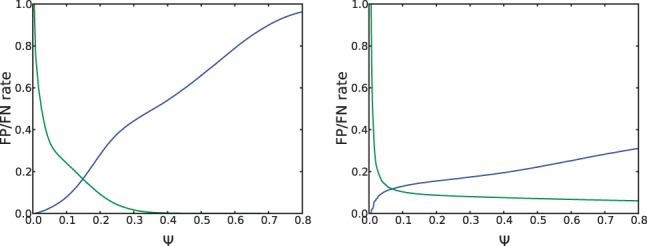
Plots of the false-positive (green) and false-negative (blue) rates for (a) B.facium and (b) S.aureus paired-end libraries

3.4.2 The decision rule

Our analysis revealed that varying parameters C and Θ within specified ranges (see Section 3 of the Appendix) hardly affects the quality of the resulting assemblies. However, selecting inappropriate C and Θ may result in a deteriorated performance of exSPAnder. Thus, we arbitrarily select these parameters within the ranges specified in Section 3 of Appendix (analysis of diverse sequencing datasets supports the default values C = 1.5 and Θ = 0.5).

4 RESULTS

4.1.1 Datasets

We have compared exSPAnder (coupled with SPAdes assembler) with several popular assemblers on the B.faecium isolate dataset (genome size 3.6 Mb) and the S.aureus single-cell dataset (genome size 2.9 Mb). For each dataset we have generated assemblies of (i) only paired-end library and (ii) both paired-end and jumping libraries. Section 1 of Appendix provides a detailed description of both datasets.

4.1.2 Benchmarking assemblies

ABySS 1.3.6, Ray 2.0.0, Velvet, Velvet-SC and SOAPdenovo 2.0.4 were run with k-mer size 55. IDBA-UD 1.1.1 was run in its default iterative mode. The authors of (Peng et al., 2012) released this new version of IDBA-UD that is capable of using several paired-end libraries, but there is no manuscript yet covering this new development. ALLPATHS-LG was run with the default parameters; however, we down-sampled jumping library for the B.faecium dataset to generate 100× coverage required by ALLPATHS-LG. SPAdes 2.4 (previous version of SPAdes that did not include exSPAnder and did not support multiple libraries) was run in its default iterative mode with k = 21, 33, 55, 77 for the B.faecium dataset and k = 21, 33, 55 for the S.aureus dataset. exSPAnder (coupled with SPAdes) was run using the default parameters.

To analyze the resulting assemblies we used QUAST 2.2 (Gurevich et al., 2013) that reports various parameters including NG50 (similar to N50, but is calculated with respect to the reference genome size), the total number of contigs/scaffolds, the length of the longest assembled contig/scaffold, the number of misassemblies and the fraction of genome mapped. QUAST defines a misassembly breakpoint as a position in the contig/scaffold, such that its left and right flanking sequences either align to the reference genome over 1 kb away from each other, or overlap by > 1 kb, or align on opposite strands or different chromosomes (Gurevich et al., 2013). To compare assemblers we used both contigs and scaffolds of length exceeding 500 bp.

Tables 2 and 3 show the benchmarking results for the B.faecium isolate dataset. Interestingly, the single-cell assemblers (IDBA-UD and exSPAnder coupled with SPAdes) as well as ABySS performed well on the B.faecium isolate dataset and produced contigs with the largest NG50 in the case of a single library. While AbySS generated the assembly with the maximal genome fraction, manual inspection revealed that it reflects the specifics of ABySS and QUAST reporting (mapping each repeat to a single position in the genome) rather than real superiority of ABySS by this metric.

Table 2.

Comparison of contigs for the B.faecium isolate dataset

Assembler	NG50	Number of contigs	Largest	Number of mis	GF
Only paired-end library
ABySS	203	40	672	0	99.9
Ray	114	51	436	1	98.9
SOAPdenovo	20	333	61	0	98.8
Velvet	144	47	550	0	99.4
Velvet-SC	163	46	550	0	99.4
IDBA-UD	202	39	483	0	99.4
SPAdes 2.4	361	24	635	1	99.7
exSPAnder	380	22	672	1	99.5
Both paired-end and jumping libraries
ABySS	203	40	672	0	99.9
ALLPATHS-LG	313	21	686	0	99.5
Ray	87	88	416	2	96.8
SOAPdenovo	20	333	61	0	98.8
Velvet	103	75	242	11	99.0
Velvet-SC	253	40	545	15	99.8
IDBA-UD	207	41	483	0	99.4
exSPAnder	3268	2	3268	1	99.9

Note: NG50 is given in kb; number of contigs is the total number of contigs >500 bp; largest stands for the length (in kb) of the longest contig assembled; number of mis is the number of misassemblies; GF stands for the fraction of genome mapped given in percent. In each column, the best value is indicated in bold.

Table 3.

Comparison of scaffolds for the B.faecium isolate dataset

Assembler	NG50	Number of scaffolds	Largest	Number of mis	GF
Only paired-end library
ABySS	383	24	676	0	99.9
Ray	204	31	553	1	98.9
SOAPdenovo	477	26	724	0	99.3
Velvet	477	28	724	0	99.4
Velvet-SC	477	28	724	0	99.4
IDBA-UD	250	30	671	0	99.4
SPAdes 2.4	361	22	671	1	99.7
exSPAnder	380	22	672	1	99.5
Both paired-end and jumping libraries
ABySS	250	30	739	1	99.9
ALLPATHS-LG	3610	7	3610	1	99.5
Ray	106	75	416	2	96.8
SOAPdenovo	480	28	810	2	99.4
Velvet	2651	14	2651	78	99.1
Velvet-SC	945	102	1381	500	98.9
IDBA-UD	1002	9	1692	0	99.4
exSPAnder	3268	2	3268	1	99.9

Note: NG50 is given in kb; number of scaffolds is the total number of scaffolds >500 bp; largest stands for the length (in kb) of the longest scaffold assembled; number of mis is the number of misassemblies; GF stands for the fraction of genome mapped given in percent. In each column, the best value is indicated in bold.

In the case of two libraries, exSPAnder produced the best contigs while ALLPATHS-LG produced the best scaffolds. The complexity of using jumping libraries is reflected in a deteriorated performance of ABySS and Ray (reduction in NG50) as well as Velvet and Velvet-SC (dramatic increase in the number of misassemblies).

Tables 4 and 5 compare various assemblers on the S.aureus single-cell dataset. This comparison highlights the complexity of both (i) assembling single-cell datasets and (ii) using jumping libraries. For example, SOAPdenovo produced assemblies of poor quality for single-cell data (we decided not to include it in Tables 4 and 5). Similarly, ABySS produced assemblies with high number of misassemblies for the single-cell data. Velvet and Velvet-SC are not included in the benchmark experiment for jumping libraries testing because they also produce low-quality assemblies when both paired-end and jumping libraries are used simultaneously. IDBA-UD performed well on a single paired-end library, but produced an assembly of lower quality when both libraries were provided (decreased NG50). exSPAnder produced assemblies with the highest NG50 and largest assembled contig/scaffold.

Table 4.

Comparison of contigs for the S.aureus single-cell dataset

Assembler	NG50	Number of contigs	Largest	Number of mis	GF
Only paired-end library
ABySS	27	914	91	262	98.0
Ray	21	306	108	14	88.7
Velvet	10	538	56	2	93.2
Velvet-SC	9	616	56	4	94.2
IDBA-UD	75	390	161	7	98.6
SPAdes 2.4	98	400	230	8	99.1
exSPAnder	148	366	275	3	98.6
Both paired-end and jumping libraries
ABySS	27	914	91	262	98.0
ALLPATHS-LG	15	283	75	26	79.9
Ray	100	178	486	21	93.5
IDBA-UD	47	415	161	7	98.6
exSPAnder	314	322	603	9	99.3

Note: NG50 is given in kb; number of contigs is the total number of contigs >500 bp; largest stands for the length (in kb) of the longest contig assembled; number of mis is the number of misassemblies; GF stands for the fraction of genome mapped given in percent. In each column, the best value is indicated in bold.

Table 5.

Comparison of scaffolds for the S.aureus single-cell dataset

Assembler	NG50	Number of scaffolds	Largest	Number of mis	GF
Only paired-end library
ABySS	28	910	91	270	98.2
Ray	21	306	108	14	88.7
Velvet	10	538	56	2	93.2
Velvet-SC	10	620	56	5	94.2
IDBA-UD	88	382	161	8	98.2
SPAdes 2.4	99	391	230	8	99.2
exSPAnder	148	357	426	4	98.6
Both paired-end and jumping libraries
ABySS	30	852	91	275	98.0
ALLPATHS-LG	40	165	132	69	79.9
Ray	100	169	486	25	93.5
IDBA-UD	55	397	161	9	98.6
exSPAnder	314	302	603	9	99.3

Note: NG50 is given in kb; number of scaffolds is the total number of scaffolds >500 bp; largest stands for the length (in kb) of the longest scaffold assembled; number of mis is the number of misassemblies; GF stands for the fraction of genome mapped given in percent. In each column, the best value is indicated in bold.

Using only paired-end library IDBA-UD, SPAdes 2.4 and exSPAnder recovered the largest fraction of the genome (>98.5%). However, the highest genome fraction of the assembly generated by SPAdes 2.4 reflects the specifics of SPAdes 2.4 and QUAST reporting (some artifacts with reporting of repetitive regions) rather than real advantage of SPAdes 2.4 with respect to this parameter.

When using both libraries simultaneously, exSPAnder produced assemblies with the highest genome fraction exceeding 99%, the largest genome fraction we saw across dozens of single-cell datasets assembled with SPAdes in the past 2 years. Moreover, Tables 4 and 5 show that exSPAnder successfully deals with the high rate of the chimeric read-pairs and relatively high variations in the insert size.

5 CONCLUSION

We have presented exSPAnder algorithm for resolving repeats using either a single or multiple read-pair libraries with different insert sizes, which is applicable for both single-cell and isolate bacterial datasets. Benchmarks across eight popular assemblers demonstrate that exSPAnder produces high-quality assemblies for datasets of different types. Additionally, as illustrated by recent integration of Illumina and PacBio reads in SPAdes 3.0, exSPAnder is a flexible approach that can be easily modified to work with diverse types of sequencing data.

REFERENCES

- Bankevich A, et al. SPAdes: a new genome assembly algorithm and its applications to single-cell sequencing. J. Comput. Biol. 2012;19:455–477. doi: 10.1089/cmb.2012.0021. [DOI] [PMC free article] [PubMed] [Google Scholar]
- Boisvert S, et al. Ray: simultaneous assembly of reads from a mix of high-throughput sequencing technologies. J. Comput. Biol. 2010;17:1519–1533. doi: 10.1089/cmb.2009.0238. [DOI] [PMC free article] [PubMed] [Google Scholar]
- Bresler M, et al. Telescoper: de novo assembly of highly repetitive regions. Bioinformatics. 2012;28:311–317. doi: 10.1093/bioinformatics/bts399. [DOI] [PMC free article] [PubMed] [Google Scholar]
- Butler J, et al. ALLPATHS: de novo assembly of whole-genome shotgun microreads. Genome Res. 2008;18:810–820. doi: 10.1101/gr.7337908. [DOI] [PMC free article] [PubMed] [Google Scholar]
- Chitsaz H, et al. Efficient de novo assembly of single-cell bacterial genomes from short-read data sets. Nat. Biotechnol. 2011;29:915–921. doi: 10.1038/nbt.1966. [DOI] [PMC free article] [PubMed] [Google Scholar]
- Compeau F, et al. How to apply de Bruijn graphs to genome assembly. Nat. Biotechnol. 2011;29:987–991. doi: 10.1038/nbt.2023. [DOI] [PMC free article] [PubMed] [Google Scholar]
- Diep B, et al. Complete genome sequence of USA300, an epidemic clone of community-acquired meticillin-resistant Staphylococcus aureus. Lancet. 2006;367:731–739. doi: 10.1016/S0140-6736(06)68231-7. [DOI] [PubMed] [Google Scholar]
- Gnerre S, et al. High-quality draft assemblies of mammalian genomes from massively parallel sequence data. Proc. Natl Acad. Sci. USA. 2011;108:1513–1518. doi: 10.1073/pnas.1017351108. [DOI] [PMC free article] [PubMed] [Google Scholar]
- Gurevich A, et al. QUAST: quality assessment tool for genome assemblies. Bioinformatics. 2013;29:1072–1075. doi: 10.1093/bioinformatics/btt086. [DOI] [PMC free article] [PubMed] [Google Scholar]
- Langmead B, Salzberg S. Fast gapped-read alignment with bowtie 2. Nat. Methods. 2012;9:357–359. doi: 10.1038/nmeth.1923. [DOI] [PMC free article] [PubMed] [Google Scholar]
- Lapidus A, et al. Complete genome sequence of Brachybacterium faecium type strain (Schefferle 6-10) Standards Genomic Sci. 2009;1:3–11. doi: 10.4056/sigs.492. [DOI] [PMC free article] [PubMed] [Google Scholar]
- Li R, et al. De novo assembly of human genomes with massively parallel short read sequencing. Genome Res. 2010;20:265–272. doi: 10.1101/gr.097261.109. [DOI] [PMC free article] [PubMed] [Google Scholar]
- Nurk S, et al. Assembling single-cell genomes and mini-metagenomes from chimeric MDA products. J. Comput. Biol. 2013;20:1–24. doi: 10.1089/cmb.2013.0084. [DOI] [PMC free article] [PubMed] [Google Scholar]
- Medvedev P, et al. Paired de bruijn graphs: a novel approach for incorporating mate pair information into genome assemblers. J. Comput. Biol. 2011;18:1625–1634. doi: 10.1089/cmb.2011.0151. [DOI] [PMC free article] [PubMed] [Google Scholar]
- Peng Y, et al. IDBA-UD: a de novo assembler for single-cell and metagenomic sequencing data with highly uneven depth. Bioinformatics. 2012;28:1–8. doi: 10.1093/bioinformatics/bts174. [DOI] [PubMed] [Google Scholar]
- Pevzner PA, et al. An Eulerian path approach to DNA fragment assembly. Proc. Natl Acad. Sci. USA. 2001;98:9748–9753. doi: 10.1073/pnas.171285098. [DOI] [PMC free article] [PubMed] [Google Scholar]
- Pham S, et al. Pathset graphs: a novel approach for comprehensive utilization of paired reads in genome assembly. J. Comput. Biol. 2013;20:259–371. doi: 10.1089/cmb.2012.0098. [DOI] [PMC free article] [PubMed] [Google Scholar]
- Simpson J, et al. ABySS: a parallel assembler for short read sequence data. Genome Res. 2009;19:1117–1123. doi: 10.1101/gr.089532.108. [DOI] [PMC free article] [PubMed] [Google Scholar]
- Vyahhi N, et al. From de Bruijn graphs to rectangle graphs for genome assembly,” in Workshop on Algorithms in Bioinformatics 2012. Lecture Notes Comput Sci. 2012;7534:200–212. [Google Scholar]
- Zerbino DR, Birney E. Velvet: algorithms for de novo short read assembly using de Bruijn graphs. Genome Res. 2008;18:821–829. doi: 10.1101/gr.074492.107. [DOI] [PMC free article] [PubMed] [Google Scholar]