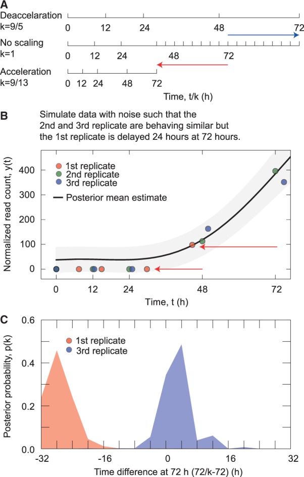
Fig. 2.

Modeling differentiation dynamics. (A) An illustration showing the effects of the time scaling. The axis in the center panel shows the unscaled time axis. The axes in the top and bottom panels show the maximum allowed deceleration (−32 h at 72 h) and acceleration (32 h at 72 h) relative to the unscaled case, respectively. (B) The estimated smooth representation of the simulated data with the time scaling. The first replicate is a delayed version of the second and third replicates. The red arrows illustrate how much the measurements are effectively moved due to the time scaling. (C) The posterior distribution of the time differences at timepoint 72 h