Inferring gene ontologies from pairwise similarity data

Abstract

Motivation: While the manually curated Gene Ontology (GO) is widely used, inferring a GO directly from -omics data is a compelling new problem. Recognizing that ontologies are a directed acyclic graph (DAG) of terms and hierarchical relations, algorithms are needed that:

1. analyze a full matrix of gene–gene pairwise similarities from -omics data;

2. infer true hierarchical structure in these data rather than enforcing hierarchy as a computational artifact; and

3. respect biological pleiotropy, by which a term in the hierarchy can relate to multiple higher level terms.

Methods addressing these requirements are just beginning to emerge—none has been evaluated for GO inference.

Methods: We consider two algorithms [Clique Extracted Ontology (CliXO), LocalFitness] that uniquely satisfy these requirements, compared with methods including standard clustering. CliXO is a new approach that finds maximal cliques in a network induced by progressive thresholding of a similarity matrix. We evaluate each method’s ability to reconstruct the GO biological process ontology from a similarity matrix based on (a) semantic similarities for GO itself or (b) three -omics datasets for yeast.

Results: For task (a) using semantic similarity, CliXO accurately reconstructs GO (>99% precision, recall) and outperforms other approaches (<20% precision, <20% recall). For task (b) using -omics data, CliXO outperforms other methods using two -omics datasets and achieves ∼30% precision and recall using YeastNet v3, similar to an earlier approach (Network Extracted Ontology) and better than LocalFitness or standard clustering (20–25% precision, recall).

Conclusion: This study provides algorithmic foundation for building gene ontologies by capturing hierarchical and pleiotropic structure embedded in biomolecular data.

Contact: tideker@ucsd.edu

1 INTRODUCTION

Ontologies have proven very useful for capturing and organizing knowledge as a hierarchical set of terms and their interrelationships. In biology, one of the most successful and widely used ontologies is from the Gene Ontology (GO) project, a major effort to represent gene functions in cellular level processes across organisms (Ashburner et al., 2000; Gene Ontology Consortium, 2001). GO is ‘the default source of functional annotations for virtually every experimental system and the gold standard for measuring the success of bioinformatic methods’ (Dolinski and Botstein, 2013). It is extensively used by researchers in a wide variety of situations, such as understanding the function of genes discovered in a Genome Wide Association Study (Holmans et al., 2009; Wang et al., 2010) or computationally predicting functions for uncharacterized genes (Pena-Castillo et al., 2008; Yan et al., 2010).

An important feature of GO is that the ontology structure is constructed by a diverse team of scientists according to their best abilities to curate the published scientific literature. As the amount of cell biological literature increases, however, curating the ontology structure has become a painstaking effort that is proving difficult to scale up and systematize (Alterovitz et al., 2010). Moreover, human curation necessarily favors biological entities that have been well studied and misses the large proportion of cell biology that is not yet known or has not yet been curated. For these reasons, it is not possible to directly learn about an uncharacterized gene or discover a new function using GO, and one cannot quickly assemble an ontology model for a new organism, let alone a specific cell type or disease state.

Recently, it has been shown by some of us that a GO can be inferred directly from molecular data as a complement to further curation efforts (www.nexontology.org) (Dutkowski et al., 2013). For ontology curators, this approach ‘is extremely valuable in three ways. First … it finds connections missed by curators. Second, it will save huge amounts of curation time by pointing curators to the data that matter. Third, it provides a quality-control check on the GO that is unbiased by the vagaries of publication policies, as it is based only on the data themselves' (Dolinski and Botstein, 2013). Furthermore, the ability to rapidly generate ontologies from data opens up new possibilities for the use of ontologies in general. ‘For example, data-driven ontologies generated from diseased and normal samples could be compared. This would be a novel way to look at what goes awry in particular disease states, providing the context and perspective of complex, interrelated biological processes’ (Dolinski and Botstein, 2013). Such an ontology model may also serve as the basis for an intelligent, predictive agent, as one of us has described elsewhere (Carvunis and Ideker, 2014). Despite these possibilities inspired by an initial attempt (Dutkowski et al., 2013) it remains an open question as to how best algorithmically to infer an ontology from molecular data.

To understand the challenges involved in inferring an ontology from data, we first must recognize that ontologies contain both syntactic information (terms and their structural relations) as well as semantic information (relations between terms have defined meanings—in GO these include ‘is a’, ‘part of’ and ‘regulates’ relations). Both our previous work and this work will focus on inferring the syntactic information—the ontology terms, their relations and the annotations of genes to terms. This syntactic information is the most commonly used information by biologists using GO as a gold standard.

GO is structured as a rooted, directed acyclic graph (DAG), where gene annotations propagate up the hierarchy from child terms to parent terms through ‘is a’ and ‘part of’ relations. For example, in the biological process (BP) branch, ‘M phase of mitotic cell cycle’ and ‘interphase of mitotic cell cycle’ are child terms beneath ‘mitotic cell cycle’. Since GO is a DAG, any term can have multiple parents and/or multiple children. Allowing for multiple children per term is necessary to capture the biological truth that many molecular machines have more than two subunits, or that a BP such as the interphase of cell cycle can be split into more than two phases (G1, S, G2). Multiple parents are necessary to capture the biological principle of pleiotropy—the reuse of genes and/or subunits, or the classification of a BP into multiple higher categories of process (e.g. ‘Sulfur Amino Acid Metabolic Process’ is a child of both ‘Cellular Amino Acid Metabolic Process’ and ‘Sulfur Compound Metabolic Process’). In order to faithfully infer an ontology of genes like GO, we need an algorithm able to infer a DAG.

In previous work, we developed a multistep algorithm for constructing a Network Extracted Ontology (NeXO), which infers a DAG structure from data summarized in the form of a molecular interaction or gene similarity network (Dutkowski et al., 2013). This algorithm first infers a binary tree using the HAC-ML algorithm (Park and Bader, 2011). Then, splits without network support are collapsed, creating nodes with more than 2 children. Finally, a post-processing step searches for additional parent–child relationships between existing nodes, allowing for a single node to have multiple parents.

The NeXO algorithm does not use quantitative information about gene interaction or similarity, i.e. it assumes an input network for which the edges are unweighted. However, typical genome-scale data such as gene expression correlation populate a full matrix of similarity scores between pairs of genes where all of the information is contained in the weights. While thresholding these data is one way to interpret them as unweighted networks, this results in information loss not only below but also above the threshold, as hierarchical structure embedded in the weights is collapsed. Furthermore, when combining multiple types of data (as will be undoubtedly required for construction of a complete ontology of gene function), it is useful to give greater weight to gene pairs which have evidence of similarity in multiple datasets (Kim et al., 2014). Since the NeXO algorithm is unable to use valuable information contained in the weights of edges in an input network, it is instead forced to rely on setting a proper threshold below which all information is ignored and above which relative weights are lost.

The essence of the DAG inference problem is to detect communities of genes that span a wide range of sizes/scales and can nest hierarchically as well as share arbitrary subsets of members. Furthermore, the algorithm should be able to construct a DAG using the information contained in weighted networks, and it should be capable of operating on a nearly complete, weighted graph with a genome-scale number of nodes (thousands) and edges (millions). A number of existing clustering algorithms address parts of this challenge. For example, there are many commonly used hierarchical clustering algorithms which use similarity or distance scores as input and infer a nested hierarchy of clusters (Florek et al., 1951; Sneath and Sokal, 1973; Sokal and Michener, 1958; Sørensen, 1948; Ward, 1963). These methods, however, rely on iterative joining of pairs of terms, resulting in forced construction of a binary tree. Clusters cannot overlap (i.e. have multiple parents for a single node) or have >2 children, and the number of clusters inferred is fixed at n −1 where n is the number of terminal nodes.

There have recently been a handful of algorithms which construct hierarchies with overlapping clusters, by creating a first level of overlapping clusters with terminal nodes and then combining these base clusters into higher level clusters (Becker et al., 2012; Kovacs et al., 2010; Kumpula et al., 2008; Sales-Pardo et al., 2007). These algorithms all present solutions that allow multiple parents and multiple children at the initial level of clusters, and some operate on weighted networks. However, these methods restrict each higher level cluster to having a single parent. This aspect inherently limits the types of relations that can be discovered by these methods.

Another relevant method has been proposed that hierarchically clusters links in a graph rather than edges (Ahn et al., 2010). This method is quite flexible and allows for each node in the graph to appear in multiple clusters via participation in multiple edges. Such a method still restricts the types of clusters it creates, however. First, an edge can only participate in a single cluster at each level of the hierarchy (although a pair of nodes may incidentally participate in multiple clusters via other edges). Secondly, the hierarchical clustering of the edges allows only for binary joins between edges and therefore each lower level cluster will be joined with exactly one other cluster at each step. This process creates e −1 clusters, where e is the number of edges in the input graph. While the original paper proposes a method for determining a single optimal cut in the hierarchy for determining clusters, how to determine all levels of the hierarchy that are meaningful and not an artifact of construction remains an open question.

The LocalFitness algorithm, which has recently been proposed in the physics community, is to our knowledge the only previous approach that constructs a DAG from an unweighted or weighted network and has a principled way of determining which clusters are robust (Lancichinetti et al., 2009). This method constructs clusters at a given level in the hierarchy by optimizing a fitness function for each of many potentially overlapping clusters built out from multiple seed nodes. The fitness function includes a parameter that is tuned to find clusters at multiple levels of the hierarchy. Graph partitionings that are stable across comparatively wide ranges of this parameter are used.

Here we present a basic formulation of the ontology inference problem followed by a description of a new method, called Clique Extracted Ontology (CliXO), for ontology inference based on progressive identification of maximal cliques. We evaluate CliXO in comparison with LocalFitness as well as several other methods such as the NeXO algorithm and standard clustering. Methods are evaluated based on their ability to reconstruct the GO from two starting datasets: (a) pairwise semantic similarities, which are derived directly from GO itself, and (b) three different -omics datasets (genetic interaction profile correlation, gene expression correlation and an integrated -omics dataset for yeast).

2 METHODS

2.1 Basics

Define an ontology-graph as a weighted DAG G = [T, N, E, w, r] with the following properties:

• The nodes in G are terminal (set T; no outgoing edges), or non-terminal (set N). Non-terminal nodes in the ontology are also called terms. G has a single root r ∈ N from which all nodes can be reached.

• Ultrametric property: a non-terminal node u in G has constant distance, denoted w(u), to all its terminal descendants, denoted by L(u).

• Witness property: for non-terminal node u, and all terminal nodes a ∉ L(u), there exists b ∈ L(u) such that w(a, b) > 2w(u).

• |G| is the total number of non-terminal nodes in G.

• For any pair of terminal nodes a, b, let w(a, b) denote the shortest path between a, b in G.

• Define a Least Common Ancestor lca(a, b) such that w(a, b) = 2w(lca(a, b)).

Figure 1A shows an example of an ontology graph, with non-terminal nodes 0, … , 6 and terminal nodes A, … , H. This model of an ontology allows for the grouping of elements (terminal nodes) into coherent clusters of elements (i.e. non-terminal nodes) that are closer to each other than to other nodes based on pairwise distances between elements.

Fig. 1.

CliXO method. (A) An example ontology with genes A–H and terms 0–6. (B) Semantic similarity scores calculated from the ontology in (A). (C) Example showing reconstruction of the ontology in (A) from the similarity scores in (B). As the threshold is decreased, edges that equal or exceed the threshold are added to the graph. At each new threshold, maximal cliques in the graph, corresponding to terms are found and added to the inferred ontology

2.1.1 The Ontology DAG reconstruction problem (perfect case)

Input: —

A set of terminal nodes (i.e. genes) T, and a distance matrix M between all pairs in M (as shown in Figure 1B).

Output: —

An ontology-graph G with T as the set of terminal vertices and for all a, b ∈ T, w(a, b) = M(a, b).

The input distances M rarely satisfy the ontology distances perfectly and therefore, in the imperfect case, we must compute the ontology DAG that best represents M.

2.1.2 The Ontology DAG reconstruction problem (imperfect case)

Input: —

A set of terminal nodes (i.e. genes) T, a distance matrix M between all pairs and a user-provided noise parameter α.

Output: —

An ontology-graph G with T as the set of terminal vertices, and which maximizes |G| while satisfying the following:

1. For all a, b ∈ T, w(a, b) ≥ M(a, b).

2. For non-terminal node u, and all terminal nodes a ∉ L(u), there exists b ∈ L(u) such that M(a, b) > 2w(u) + α.

3. For each non-terminal node u, there must be at least one pair of terminal nodes a, b ∈ L(u) for which 2w(u) + α < 2w(v) for all v with a, b ∈ L(v), v ≠ u.

4. For all u ∈ N, w(u) = 2 max_{a,b ∈ L(u)} M(a, b)

2.1.3 Distance versus similarity scores

We note that in many cases, the relationship between terms is presented in the form of a similarity matrix, rather than a distance matrix. The two are interchangeable for the algorithms proposed below. For example, subtract the similarity scores from a large constant to get a valid distance function between two terms.

2.2 CliXO algorithm

We consider a simple heuristic as described in Figure 1C. Consider an undirected graph U with nodes ∈ T and no edges. Let S be a stack of all pairs (a, b) sorted by distances M(a, b), with the smallest value at the top.

Algorithm CLIXO(S).

Input: Stack S of sorted distances

Output: Non-terminal nodes in the ontology-graph

1. C_G = {}

2. while (S ≠ {})

3. (a, b) = top(S); t = M(a, b)

4. while (M(a, b) == t)

5.  (a, b) = Pop(S)

6.  Add edge (a, b) to U

7. C_cur = Set of maximal cliques in U

8. C_G = C_G ∪ C_cur

9. (C_G forms the set of non-terminal nodes in G)

Note that each maximal clique in U corresponds to a node of the ontology graph, with an obvious hierarchy. We use an algorithm proposed by Chiba and Nishizeki (1985) to compute all maximal cliques in time O(mμ a(U)) where m is the number of edges in U, μ is the number of maximal cliques in U and a(U) is the arboricity of U (a(U) < n where n = |T|). While output-efficient, the number of cliques can be large. Moreover, the algorithm may output the same cliques repeatedly.

We modify the algorithm above to maintain only informative maximal cliques defined as follows. At any time in the algorithm, a pair of terminal nodes a, b is explained if a and b are both elements of a single clique which is already in C_G. A clique is necessary if it contains a pair of terminal nodes c, d which is not contained in any other single clique in C_cur. A clique C ∈ C_cur is informative if it is both necessary and contains at least one pair of non-explained terms. Only informative cliques are added to C_G.

Next, we check cliques dynamically for maximality and informativeness. Define N(a) as the set of vertices adjacent to a in U. Let C_a represent the set of maximal cliques in C_cur containing a. Consider Steps 5 and 6, where (a, b) is popped off S and edge (a, b) is added to U. For each clique C′ ∈ C_a, we create a new clique C′ ∩ N(b) ∪ {b}. Similarly, for each clique C′ ∈ C_b, we will create a new clique C′ ∩ N(a) ∪ {a}. These are the only new cliques. Each new clique C_new is checked for maximality. If maximal, add each C_new to C_cur, and remove from C_cur all cliques in C_a or in C_b that are contained in (i.e. a subset of) a C_new. Finally, when we are ready to increase the threshold [all (a, b) matching the current threshold have been popped], we check all cliques in C_cur and retain only the informative ones. CliXO with dynamic checking for maximality and informativeness can compute all informative maximal cliques in O(Mnγ) where M is the number of non-zero edges in M, n = |T| and γ is the number of informative cliques in the final output G. Practically, γ ≪ μ, where μ is the total number of all maximal cliques at each unique t in U, and this results in significant performance increase.

2.2.1 Imperfect case

In the imperfect case, the only change is in Step 8 of the CliXO algorithm. Instead of adding all informative cliques in C_cur to C_G each time a new threshold is reached, we add to C_G only those informative cliques C in C_cur for which max_{a,b ∈ C} M(a, b) < t− α.

This algorithm can perfectly distinguish between signal and noise when α is smaller than s, the smallest distance between any child–parent node pair in the ontology and larger than a noise value n(G), determined by the following procedure. For each term u ∈ G, order by value all M(a, b) where a, b ∈ u. n(u) for a non-terminal node u is the maximum difference between adjacent values in this ordered list and n(G) = max_u∈N n(u). It is not possible to directly determine n(G) without knowing the true ontology structure, but it is a useful concept for understanding α. On a conceptual and practical level, n(G) can be estimated as roughly 2× the standard error of measured pairwise distances (e.g. when the experiments used to measure distance are replicated both technically and biologically). α can be set to this estimated n(G).

It may not always be possible to set α so that n(G) < α < s because sometimes n(G) > s. In this case, if α < n(G), it will result in the creation of extraneous terms that are a subset of a ‘real’ term. If α > s then any ‘real’ child node c that is close to its parent node p, i.e. 2(w(p) − w(c)) < α, will not be included in the ontology. One practical strategy for dealing with this case is for the user to focus on a particular small, well-known section of the ontology (e.g. a molecular machine like the proteasome) and observe it over various levels of α. If many extraneous terms seem to be being created, then α is likely too low. If known levels of the hierarchy are being collapsed, then α is likely too high.

2.2.2 Missing edges (false negatives)

We expect that in real molecular data, there will be a number of missing edges—i.e. measurements for a, b ∈ T where M(a, b) ≫ w(a, b) in the ‘true’ ontology. These missing edges will cause splitting of maximal cliques into highly overlapping smaller cliques. For example, a ‘true’ term of size k with just one missing edge in the measured distances M will result in two smaller terms of size k + 1 in the DAG inferred from M.

2.2.3 Algorithm: Missing Edges

We maintain the properties of the noisy measurements case. However, we now add a user-defined parameter β and the ability to edit M, the input distance matrix, when we infer that an edge is likely missing (i.e. is a false negative). β is a parameter where 0 < β ≤ 1. Two cliques C_i and C_j are considered highly overlapping by the algorithm if for all a ∈ C_i ∪ C_j, $\frac{\left|N(a)\cap (C_i\cup C_j)\right|}{|C_i\cup C_j|-1}\ge \mathrm{\beta .}$We modify the CliXO algorithm, again in Step 8. Before an informative, maximal clique C_i ∈ C_cur is added to C_G, we check all other C_j ∈ C_cur for high overlap with C_i. For any C_j found to be highly overlapping with C_i, we also check for any C_k ∈ C_cur that are highly overlapping with C_j. Recall w(C) = max_a,b∈C M(a, b). For all such highly overlapping pairs of cliques C_i and C_j, we then set M(a, b) = max(w(C_i), w(C_j)) for all a, b ∈ (C_i ∪ C_j) with M(a, b) > max(w(C_i), w(C_j)). We add all edges adjusted in M to U and update C_cur.

2.2.4 Other algorithms considered

We evaluate ontologies inferred using the NeXO algorithm (Dutkowski et al., 2013), the Local Fitness Algorithm (Lancichinetti et al., 2009), and several standard hierarchical clustering algorithms including the Unweighted Pairwise Group Method (UPGMA; Sokal and Michener, 1958), the Weighted Pairwise Group Method (WPGMA; Sneath and Sokal, 1973), Ward’s minimum variance method (Ward, 1963), Complete Linkage (Sørensen 1948), and Single Linkage (Florek et al., 1951).

2.3 Evaluation of reconstructed ontologies

2.3.1 Ontology alignment

Ontologies were aligned as in Dutkowski et al. (2013). Briefly, given two ontologies O₁ with n₁ terms and O₂ with n₂ terms, an ontology alignment A is a mapping of terms between ontologies such that each term in O₁ maps to at most one term in O₂ and vice versa. Term mapping in our alignment procedure is evaluated using a score function that considers the similarity of the sets of genes assigned to terms (intrinsic similarity) and the similarity of the ontology hierarchy surrounding each term (relational similarity). Each pair of terms which is aligned receives an alignment score ranging from 0 to 1 where 1 represents identity in both intrinsic and relational similarity.

To calculate false discovery rate (FDR) of term alignment, we first create n ontologies with the same structure as the inferred ontology O_i but with all gene labels randomly permuted. The FDR of a term alignment at a given score t is then:

$$\text{FDR}(t)=\frac{\frac{1}{n}{\displaystyle \sum _{i=1}^n{N}_{R_i}(t)}}{N(t)}$$

Where $N_{R_i}(t)$ is the number of terms in the random permutation i that have an alignment score ≥t, and N(t) is the number of terms in the ontology O_i that have an alignment score ≥t. Terms are binned by size for the FDR computation, and we set a minimum score threshold value t ≥ 0.1 for large terms and higher threshold values for small terms so as to maintain an FDR <5% within each size group.

The alignment procedure also respects the preservation of structural relationships across ontologies being aligned. It does this by ensuring that there are no conflicts between individual mappings in the final alignment. There are two versions of the alignment—in the permissive version, a conflict exists between mappings (e₁, e₂) and (e₁′, e₂′) where e₁, e₁′ ∈ O₁ and e₂, e₂′ ∈ O₂ if there is a parent–child criss-cross—that is, either e₁ is a descendant of e₁′ in O₁ and e₂ is an ancestor of e₂′ in O₂, or e₁′ is a descendant of e₁ in O₁ and e₂′ is an ancestor of e₂ in O₂. In the strict version, there is a conflict if e₁ is a descendent of e₁′ in O₁ and e₂ is not a descendent of e₂′ in O₂. The permissive version places most value on the alignment between individual nodes, whereas the strict version also requires that the relations between nodes are preserved.

2.3.2 Precision and recall of inferred ontologies

For evaluating inferred ontologies, we first align the inferred ontology I to the gold standard ontology G, in our case GO. This gives us an alignment A. We then determine precision and recall as

$$\text{precision}=\frac{\left|A\right|}{\left|I\right|},\text{recall}=\frac{\left|A\right|}{\left|G\right|}$$

where |A| is the number of terms aligned with t ≥ 0.1 and FDR <5%.

3 RESULTS AND DISCUSSION

3.1 Ontology inference from semantic similarity

We began by testing performance using input similarity data that are perfectly consistent with the target ontology. For this task, we calculated the Resnik semantic similarity (Resnik, 1995) of all gene pairs in the BP branch of GO to form a complete, weighted graph. Using these data, CliXO was able to nearly identically infer the original ontology, with >98% of BP terms identically reconstructed (Fig. 2A) and 100% of inferred terms aligned to a term in BP (Fig. 2B). The other algorithms tested, including several common hierarchical clustering methods which build trees and a method for directly creating a DAG (Local Fitness), struggled with this task by comparison. The Local Fitness algorithm, while capable of operating on a complete, weighted graph, struggles to distinguish the borders of terms, instead joining true terms into larger groups which do not recapitulate the true ontology (recall <5%, precision <30% by alignment). The hierarchical clustering methods behave similarly to each other (with the exception of single linkage which performs worse). While these methods often reconstruct BP terms (recall of ∼20% terms identical, ∼70% terms aligned), these methods suffer from the creation of numerous extra terms. Since they create a binary tree, they are forced by construction to create terms even if they are not supported by the data. This greatly damages the precision of these methods. The ontologies created by these methods contain roughly 3× as many terms as the true ontology. CliXO, on the other hand, finds the borders of each term from the data—it is not forced to create terms where they do not exist.

Fig. 2.

Inferring an ontology from semantic similarity. Precision–recall plots for ontologies inferred from GO BP Resnik semantic similarities. True positive inferred terms are identical (A) or aligned (B) to a GO BP term using permissive alignment

The NeXO algorithm, while not able to operate on a complete graph, can be run on these data by applying a threshold at a semantic similarity value and keeping only edges above this threshold. While this results in information loss, especially about larger ontology terms and substructure of smaller terms, NeXO is capable of at least approximating many terms (∼40% recall, ∼70% precision by alignment) when using a network with edges consisting of the top 10 000 semantic similarity scores (these top scores actually perfectly specify the terms of size 10 genes or fewer, as the vast majority of edges in the semantic similarity network are due to larger terms). Still, the terms produced by the NeXO algorithm are only an approximation of the true terms (precision, recall <10% by identity). Furthermore, the precision slips dramatically with almost no gain in recall as the threshold is lowered and NeXO uses more edges (recall 42%, precision 62% by alignment using the top 20 000 edges; recall 43%, precision 49% by alignment using the top 100 000 edges).

The 83 GO BP terms not identically reconstructed by CliXO are those where information loss occurs in the conversion to semantic similarities. There are two such possible cases. First, two highly overlapping terms are indistinguishable from one larger term if the genes in the overlap already belong to a term with higher similarity. For example, if {a, b, c, d} = T₁, {a, b, c, e} = T₂, {d, e} ∈ T₃, then CliXO cannot distinguish T₁ from T₂. Therefore, one term with {a, b, c, d, e} will be created. Second, a term is ‘invisible’ in the semantic similarity data if all gene pairs in that term also belong to higher similarity terms. CliXO cannot discover these ‘invisible’ terms.

3.2 Accounting for noise

Of course, we cannot expect to have experimental data that exactly model a semantic similarity measure. We expect three types of noise in experimental data—false positives, false negatives and Gaussian noise.

The simplest of these cases is false positives (cases where a gene pair is falsely assigned a high similarity). Assuming that false positives are randomly scattered throughout the network, we can expect that these false positives are unlikely to form and/or complete a clique. Rather, these will lead to the creation of small maximal cliques, usually containing only the two genes with the false positive measurement between them. In some cases, a particularly well-placed false positive may create an extraneous clique of size 3. For this reason, we choose to ignore terms of size 2 and 3 when our algorithm is run on experimental data.

Gaussian noise in measurement will cause gene pairs that all belong to the same ontology term to have slightly different measured similarities. To simulate this, we added Gaussian noise centered at 0 with varying SDs to the calculated Resnik semantic similarities and then inferred the ontology. Without the α parameter (α = 0), CliXO incorrectly infers many intermediate terms (leading to low precision, Fig. 3A) in addition to the correct terms (leading to high recall, Fig. 3B). When the α parameter is included and optimized (Section 2.2.1), then the CliXO algorithm is able to distinguish signal from noise. This allows for stable performance of CliXO even in the presence of noise. It should be noted that the median signal in this ontology is actually two orders of magnitude above the minimum signal, so even at a relative noise of 0.1, some terms in the ontology are already completely washed out due to noise. For all values where noise is less than minimum signal, CliXO with the α parameter is able to perfectly reconstruct the input ontology.

Fig. 3.

CliXO with Noise. Precision (A, C) and recall (B, D) for ontology inferred from Resnik semantic similarities beneath and including CC Biogenesis BP term (GO:0044085). True positives by strict alignment. Varying levels of Gaussian noise added to (A, B) or edges removed from (C, D) semantic similarity measure. Relative noise = 1/Median Signal to Noise ratio. Error bars represent standard error over 10 tested networks with random noise or edges removed per point

False negatives are cases where two genes belong to the same term but the edge between them either does not exist or has an extremely small similarity. The effect of a missing edge from a clique of size k genes is to split that clique into two smaller cliques of size k − 1 genes that share k − 2 genes. To account for these missing edges, our method incorporates the parameter β which causes the algorithm to find and merge highly overlapping cliques (Section 2.2.3). Without this parameter (equivalent to β = 1), CliXO immediately infers far too many terms, resulting in very low precision even with only 1–10% of edges missing (Fig. 3C). With β = 0.5, CliXO is able to maintain very high precision and recall even with large percentages of edges removed (precision and recall remain >80% with half of all edges removed and >50% with 80% of all edges removed, Fig. 3C, D). It should be noted that there is a slight hit in recall by using β = 0.5 when no edges are removed—this is because there are a small number of real terms in the ontology which qualify as highly overlapping, and these terms are erroneously merged. Still, recall remains ∼90% with precision near 100%.

A thought experiment may reveal why the algorithm is robust with a fixed β over a wide range of missing edges. The operation to infer missing edges is based on finding pairs of highly overlapping cliques and filling in missing edges between them. If a single edge is missing from an otherwise complete clique C, this will create two highly overlapping cliques C₁, C₂ ⊂ C which will each contain one unique element. C₁ and C₂ will be merged by the algorithm to create C. If a second edge is removed which does not share a vertex with the first, then these two cliques will now each split into two cliques (for a total of four cliques—C₁₁, C₁₂ ⊂ C₁ and C₂₁, C₂₂ ⊂ C₂). Even if β is set so that C₁₁ is not considered highly overlapping with C₂₁ or C₂₂, still C₁₁ will first be joined with C₁₂ to form C₁ while C₂₁ and C₂₂ are joined to form C₂. C₁ and C₂ will then be found to be highly overlapping and are therefore joined to make C. As more edges are removed from the original clique C this will simply lead to extra rounds of clique merging before C is recovered (this breaks down a bit as missing edges share vertices, but with a β set appropriately low this can be overcome). Because of this thought experiment and the experimental results in Figure 3C and D where the algorithm displays robustness to a wide range of missing edges with β = 0.5, we have set β = 0.5 for all experiments using -omics data. We recommend this setting for all use cases where missing edges are expected.

3.3 Ontology inference from -omics data for yeast

With CliXO performing well even in the presence of noise and significant levels of false negatives, we turned to the problem of inferring an ontology directly from experimental data. For this purpose, we used three -omics datasets—genetic interaction (GI) profile Pearson correlations as provided by Costanzo et al. (2010), gene expression (GE) profile correlations across all arrays in the Stanford Microarray Database (Hubble et al., 2009) and YeastNet v3 (Kim et al., 2014), a recently released functional gene network which combines evidence from multiple experimental sources to provide a weighted functional relationship between genes. All three of these datasets provide quantitative weights that correlate with the semantic similarities calculated from GO BP (Fig. 4A, C and E).

Fig. 4.

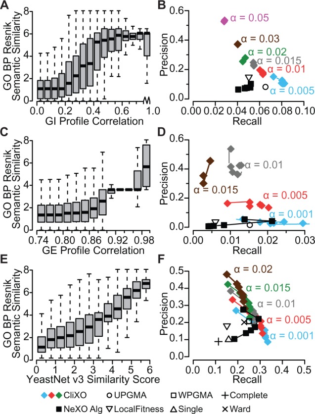
Inferring an Ontology from -omics data. (A, C, E) Pairwise similarity scores from data versus BP Resnik Semantic Similarity. A = Genetic Interaction (GI) profile Pearson correlation as provided by Costanzo et al. (2010); C = Gene expression (GE) Pearson correlation from Stanford Microarray Database (SMD); E = YeastNet v3. (B, D, F) Precision–recall plot for ontologies reconstructed using various methods and evaluated by strict alignment to GO BP. Data from GI profile correlation (B), GE profile correlation (D) or YeastNet v3 similarity (F). CliXO with varying α is shown by color change. At a given α parameter, the precision–recall curve for the CliXO ontology (terms ordered by weight at which they are inferred) is shown. NeXO results are shown with varying threshold edge weights for generating an unweighted input network

We noted that in all three of these datasets, there is a tight and strong correlation with the GO BP semantic similarity values at the very highest end. However, this tight correlation loosens as the edge weights in the -omics data decrease, as seen by wider ranges of scores and also several consecutive levels of scores indistinguishable from the lowest scores. This indicates increasing levels of false positives as the edge weights decrease. At this point we note that the CliXO algorithm outputs terms in order of decreasing weight, where a term weight is equal to the lowest similarity edge between any two genes in that term. This, combined with the decreasing reliability of the -omics data as the edge weights decrease, means that a single run of CliXO with a fixed α outputs terms in order of reliability, with the most reliable first. As such, a precision–recall curve can be calculated for a single CliXO ontology where a single point represents the alignment to GO of a CliXO ontology containing all terms above a given term weight. These precision–recall curves for CliXO at a fixed α are shown in Figure 4B, D and F, with the top left points representing a term weight equivalent to the top 10 000 edges and the bottom right point representing all terms for GI and YeastNet v3 and a term weight equivalent to the top 100 000 edges in the GE network.

We applied CliXO and several other algorithms to the problem of inferring the ontology from each of these three -omics datasets and aligned the resulting ontologies to GO BP. We report precision–recall curves for a range of α values, where lower α creates more terms and results in higher recall but at the cost of lower precision. For genetic interaction profile correlations, CliXO was the clear winner, with all α values resulting in precision–recall curves with higher precision–recall (50–10%, 3–8% by strict alignment) than competing methods including LocalFitness (15% precision, 5% recall), UPGMA (8%, 6.4%) and NeXO (10%, 5% at threshold of top 10 000 edges).

Next, several algorithms were run on the Pearson correlations of gene expression profiles across all arrays in the Stanford Microarray Database. All methods scored relatively poorly for the recall of GO BP terms (<3%). This is likely because these profiles were calculated across all arrays, causing information from individual experiments (which each represent relatively few arrays of the total) to be lost. The CliXO algorithm, however, was the only algorithm capable of separating the information present from noise, producing precision as high as >50% (Fig. 4D) for some parameter settings, greatly outperforming other algorithms (<10% precision).

We next applied all algorithms to YeastNet v3. In this test, all versions of CliXO (precision 17–41%, recall 31–21% by strict alignment) and the NeXO algorithm with an optimized threshold of the top 20 000 edges (precision ∼24%, recall ∼28% by strict alignment) outperformed other methods tested (Fig. 4F).

We note that while NeXO with an optimized threshold parameter is capable of matching CliXO in precision and recall, the performance of the NeXO algorithm is much more sensitive to this parameter choice than CliXO is to the choice of either α or a term weight threshold. In fact, the performance of the NeXO algorithm degrades quite rapidly as its threshold is loosened (Fig. 4F). Furthermore, the NeXO algorithm is quite inconsistent in its output as the threshold is varied. When compared with the best NeXO using the top 20 000 edges in YeastNet v3, no other versions of NeXO reproduced >4% of the terms exactly, and less than half of the terms aligned strictly (Fig. 5A). Without a reliable gold standard, it would be quite difficult to set this threshold for NeXO reliably.

Fig. 5.

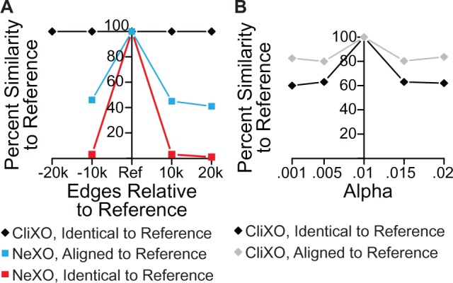
Stability of NeXO and CliXO with respect to parameters. (A) Both NeXO and CliXO algorithms run with varying numbers of edges from YeastNet v3. Reference is best performing result (20k for NeXO, 30k, α = 0.01 for CliXO). Percent similarity defined as number of terms either identical or aligned strictly divided by the number of terms in the smaller of the two ontologies produced. (B) CliXO run with varying levels of α. Reference is α = 0.01

CliXO, on the other hand, simply offers the user a tradeoff between precision and recall with its parameters. As α increases, so does precision at the cost of decreased recall. Furthermore, the CliXO algorithm is quite consistent as its parameters are varied, in contrast to the NeXO algorithm. As more terms are considered (lower edge weight threshold), all previously created terms are unaffected (Fig. 5A). Varying α also preserves the majority of terms, with >60% identical and >80% aligned strictly to CliXO with α = 0.01 (Fig. 5B). This behavior allows the user to have confidence that CliXO is producing reliable output over a range of parameter settings. Furthermore, the effect of tuning these parameters is predictable.

The CliXO inferred ontology with α = 0.01 infers 1833 terms from the top 30 000 edges in YeastNet v3 with a precision of 30% and a recall of 25% by strict alignment. The resulting structure is in fact a DAG and not a tree, as many nodes have multiple parents (Fig. 6A) and multiple children (Fig. 6B). Genes are more likely to be annotated directly to multiple parents (range 1–12, median 2) than internal nodes (range 1–3, 32 have multiple parents). Created terms range is size, roughly following a power law distribution as expected (Fig. 6C). The inferred ontology aligns not only to terms in the BP branch of GO, but also to the cellular component (CC) and Molecular Function (MF) branches. Overall, 44% of the 1833 terms in this inferred ontology align to at least one of the branches in GO at an FDR of <5% using strict alignment (Fig. 6D).

Fig. 6.

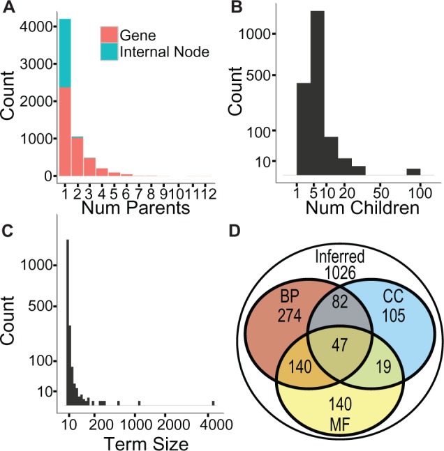
CliXO Ontology from YeastNet v3. (A–C) Statistics about CliXO inferred ontology with α = 0.01, including number of parents (A) and number of children per non-terminal node (B) and distribution of term sizes inferred (C). (D) Number of terms in CliXO inferred ontology with α = 0.01 aligned strictly with FDR <5% against all three branches of GO (CC, MF, BP). Unaligned terms in outer circle

It should be noted that YeastNet v3 learns functional relationships from data in a supervised fashion, with GO BP term comembership serving as the gold standard for training. Therefore, there is some circularity in reconstructing GO BP from this network. However, comparisons between reconstruction methods are still valid. Furthermore, the training takes place only at the level of the weight for each experiment type, so there is ample opportunity for a gene pair to score highly despite no known relationship in GO.

3.4 Further applications of CliXO algorithm

Here we have explored the de novo construction of ontologies from pairwise similarity data and compared several potential algorithms to do so. We have also introduced a new algorithm, CliXO, which performs well at this task and also may have further applications. First, CliXO may be useful as a way to combine manually curated ontologies with -omics data to create an updated ontology. For example, semantic similarities calculated from a manually curated ontology could be adjusted based on support in -omics data, followed by reconstruction of the ontology using CliXO. The updated ontology could then be aligned to and compared with the original ontology, revealing areas where -omics data supports changes to the original ontology.

Furthermore, CliXO can be viewed as a generic algorithm to convert pairwise similarity measurements between individual entities into a hierarchical DAG where terms represent groups of entities which are similar to each other and a single entity may belong to more than one term. The exact meaning of the resulting structure will change depending on the similarity measurement used, but in general there will be an intuitive understanding of the result. For example, one could take a similarity measurement between cancer patients’ genomes and then use the CliXO algorithm to construct a hierarchical DAG where each term represents a group of patients that are genetically similar to each other—i.e. genetic subtypes of cancer. As another example, one could take measurements of connection similarity in a social network and use CliXO to discover social groups in this network. We leave these applications for future work.

4 CONCLUSION

Here we have explored the requirements for inferring an ontology from a similarity matrix and available methods for doing so, as well as proposed a new method, CliXO. We found that CliXO outperforms other methods when a reliable similarity matrix is available. When using -omics data, we found that CliXO outperforms other methods on two of three datasets tested and ties the NeXO algorithm on the third, where both were able to successfully infer an ontology similar to GO BP. Furthermore, CliXO proved significantly more stable than NeXO to changes in parameters. This study provides the algorithmic foundation for building gene ontologies by capturing hierarchical and pleiotropic structure embedded in biomolecular data.

Funding: National Resource for Network Biology and the Cytoscape Project (National Institutes of Health grants P41GM103504 and R01GM070743); Department of Defense (DoD) through the National Defense Science & Engineering Graduate Fellowship (NDSEG) Program (to M.K.). VB was supported in parts by grants from the National Science Foundation (CCF-1115206 and IIS-1318386), and from the NIH (U54 HL108460, 1P01HD070494).

Conflict of Interest: none declared.

References

- Ahn YY, et al. Link communities reveal multiscale complexity in networks. Nature. 2010;466:761–764. doi: 10.1038/nature09182. [DOI] [PubMed] [Google Scholar]
- Alterovitz G, et al. Ontology engineering. Nat. Biotechnol. 2010;28:128–130. doi: 10.1038/nbt0210-128. [DOI] [PMC free article] [PubMed] [Google Scholar]
- Ashburner M, et al. Gene ontology: tool for the unification of biology. The Gene Ontology Consortium. Nat. Genet. 2000;25:25–29. doi: 10.1038/75556. [DOI] [PMC free article] [PubMed] [Google Scholar]
- Becker E, et al. Multifunctional proteins revealed by overlapping clustering in protein interaction network. Bioinformatics. 2012;28:84–90. doi: 10.1093/bioinformatics/btr621. [DOI] [PMC free article] [PubMed] [Google Scholar]
- Carvunis A, Ideker T. Siri of the cell: what biology could learn from the iPhone. Cell. 2014;157:534–538. doi: 10.1016/j.cell.2014.03.009. [DOI] [PMC free article] [PubMed] [Google Scholar]
- Chiba N, Nishizeki T. Arboricity and subgraph listing algorithms. SIAM J. Comput. 1985;14:210–223. [Google Scholar]
- Costanzo M, et al. The genetic landscape of a cell. Science. 2010;327:425–431. doi: 10.1126/science.1180823. [DOI] [PMC free article] [PubMed] [Google Scholar]
- Dolinski K, Botstein D. Automating the construction of gene ontologies. Nat. Biotechnol. 2013;31:34–35. doi: 10.1038/nbt.2476. [DOI] [PubMed] [Google Scholar]
- Dutkowski J, et al. A gene ontology inferred from molecular networks. Nat. Biotechnol. 2013;31:38–45. doi: 10.1038/nbt.2463. [DOI] [PMC free article] [PubMed] [Google Scholar]
- Florek K, et al. Sur la liaison et la division des points d'un ensemble fini. Colloq. Math. 1951;2:282–285. [Google Scholar]
- Gene Ontology Consortium. Creating the gene ontology resource: design and implementation. Genome Res. 2001;11:1425–1433. doi: 10.1101/gr.180801. [DOI] [PMC free article] [PubMed] [Google Scholar]
- Holmans P, et al. Gene ontology analysis of GWA study data sets provides insights into the biology of bipolar disorder. Am. J. Hum. Genet. 2009;85:13–24. doi: 10.1016/j.ajhg.2009.05.011. [DOI] [PMC free article] [PubMed] [Google Scholar]
- Hubble J, et al. Implementation of GenePattern within the Stanford Microarray Database. Nucleic Acids Res. 2009;37:D898–D901. doi: 10.1093/nar/gkn786. [DOI] [PMC free article] [PubMed] [Google Scholar]
- Kim H, et al. YeastNet v3: a public database of data-specific and integrated functional gene networks for Saccharomyces cerevisiae. Nucleic Acids Res. 2014;42:D731–D736. doi: 10.1093/nar/gkt981. [DOI] [PMC free article] [PubMed] [Google Scholar]
- Kovacs IA, et al. Community landscapes: an integrative approach to determine overlapping network module hierarchy, identify key nodes and predict network dynamics. PLoS One. 2010;5:e12528+. doi: 10.1371/journal.pone.0012528. [DOI] [PMC free article] [PubMed] [Google Scholar]
- Kumpula JM, et al. Sequential algorithm for fast clique percolation. Phys. Rev. E Stat. Nonlin. Soft Matter Phys. 2008;78:026109. doi: 10.1103/PhysRevE.78.026109. [DOI] [PubMed] [Google Scholar]
- Lancichinetti A, et al. Detecting the overlapping and hierarchical community structure in complex networks. New J. Phys. 2009;11:033015. [Google Scholar]
- Park Y, Bader JS. Resolving the structure of interactomes with hierarchical agglomerative clustering. BMC Bioinformatics. 2011;12(Suppl. 1):S44. doi: 10.1186/1471-2105-12-S1-S44. [DOI] [PMC free article] [PubMed] [Google Scholar]
- Pena-Castillo L, et al. A critical assessment of Mus musculus gene function prediction using integrated genomic evidence. Genome Biol. 2008;9(Suppl. 1):S2. doi: 10.1186/gb-2008-9-s1-s2. [DOI] [PMC free article] [PubMed] [Google Scholar]
- Resnik P. Using information content to evaluate semantic similarity in a taxonomy. Int. Joint Conf. Artif. 1995;1:448–453. [Google Scholar]
- Sales-Pardo M, et al. Extracting the hierarchical organization of complex systems. Proc. Natl Acad. Sci. USA. 2007;104:15224–15229. doi: 10.1073/pnas.0703740104. [DOI] [PMC free article] [PubMed] [Google Scholar]
- Sneath PH, Sokal RR. Numerical Taxonomy. The Principles and Practice of Numerical Classification. San Francisco, USA: W. H. Freeman; 1973. [Google Scholar]
- Sokal RR, Michener CD. A statistical method for evaluating systematic relationships. The University of Kansas Scientific Bulletin. 1958;38:1409–1438. [Google Scholar]
- Sørensen T. A method of establishing groups of equal amplitude in plant sociology based on similarity of species and its application to analyses of the vegetation on Danish commons. Biol. Skr. 1948;5:1–34. [Google Scholar]
- Wang K, et al. Analysing biological pathways in genome-wide association studies. Nat. Rev. Genet. 2010;11:843–854. doi: 10.1038/nrg2884. [DOI] [PubMed] [Google Scholar]
- Ward JH. Hierarchical grouping to optimize an objective function. J. Am. Stat. Assoc. 1963;58:236–244. [Google Scholar]
- Yan H, et al. A genome-wide gene function prediction resource for Drosophila melanogaster. PLoS One. 2010;5:e12139. doi: 10.1371/journal.pone.0012139. [DOI] [PMC free article] [PubMed] [Google Scholar]