Amygdala Atrophy in MCI/Alzheimer’s Disease in the BIOCARD cohort based on Diffeomorphic Morphometry

Abstract

Surface-based deformation markers obtained from diffeomorphic mapping of the amygdala are used to study specific atrophy patterns in a combined mild cognitively impaired and demented cohort compared with cognitively normal aging subjects. Statistical analysis demonstrates with high significance in a small sample of legacy data that deformation-based morphometry provides sensitive markers for locating atrophy in the amygdala. With respect to a high-field amygdala atlas, significant atrophy was found in the basomedial and lateral nucleus subregions.

Introduction

Magnetic resonance imaging (MRI) studies have substantially advanced our knowledge of brain atrophy in Alzheimer’s Disease (AD) [1]. MRI measures are an indirect reflection of the neuronal injury that occurs in the brain as the AD pathophysiological process evolves. Several MRI measures are known to be altered among individuals with AD or mild cognitive impairment (MCI), including volumetric MRI. In the initial stages of AD, atrophy appears to have a predilection for brain regions with heavy deposits of neurofibrillary tangles [2–4]. Consistent with this pattern of neurofibrillary pathology, the volume of the entorhinal cortex and hippocampus have been shown to discriminate patients with AD or MCI vs. cognitively normal subjects to be associated with the progression from MCI to AD [5].

To date, most MRI studies of subcortical gray matter nuclei have defined a single measure of structural volume [6–8]. While this has the advantage of being quantitative, it does not give specific information about subregions of atrophied nuclei. This information would be useful in order to determine whether morphometric results correlate with L. Wang, P. Yushkevich and S. Ourselin (Eds.): MICCAI 2012 Workshop on Novel Imaging Biomarkers for Alzheimer’s Disease and Related Disorders (NIBAD’12), p. 155, 2012. Copyright held by author/owner(s). neuropathologic studies, to define better the subregional distribution of atrophy, and correlate pathologic changes with clinical features of AD.

Methods of statistical shape analysis have proved enlightening for studying normal age-related changes in subcortical nuclei and for studying a number of other diseases [9–14]. We have now applied these methods to examine regional atrophy within subcortical gray matter nuclei in a cohort from the BIOCARD (“Biomarkers of Cognitive Decline Among Normal Individuals: the BIOCARD cohort”) study which is a longitudinal characterization of individuals including structural brain MRI. The BIOCARD study extends work done at the National Institute of Mental Health at NIH from 1995 to 2005. The goal is to identify bi-omarkers associated with progression from normal cognitive status to MCI or dementia, with a focus on AD.

Despite its proximity to the hippocampus, relatively little is known about the role of amygdala in MCI and AD. Following earlier histopathological findings [15–19], neuroimaging studies suggest that amygdala volume may correlate with that of the hippocampus in AD [20]. Further, recent shape analysis [21, 22] suggests there is substantial atrophy within the amygdala in AD. Thus with the expanded focus on other structures, it is opportune to perform shape analysis of the amygdala in this unique study.

Statistical shape analysis requires a preliminary alignment phase, which produces a high-dimensional representation in a fixed coordinate system. A common approach in this framework is to register all shapes to a single one, called the template, defining each anatomy by its position relative to the template. This is achieved via diffeomorphic mapping methods. It is important, in this context, to ensure that the template is as close as possible to the population, and it will be defined as the population average. Finally, the statistical analysis uses standard multivariate models, in which significance must be carefully assessed while taking multiple comparisons into account.

Methods

Data acquisition and structures

A subset of 445 scans corresponding to 173 subjects was used in this study. All subjects were cognitively normal when they were recruited. During the study period, there were a total of 155 subjects which were deemed cognitively normal by the NIH with a total of 380 scans. At the end of the period, 9 subjects were diagnosed with dementia of Alz-heimer’s type (DAT), and 9 subjects were diagnosed with MCI by the NIH. The two groups consisted of the 18 MCI/DAT subjects, and 155 cognitively normal individuals. Diagnoses made by the research team at the NIH were then confirmed using the diagnostic approach adopted by all Alzheimer’s Disease Research Centers.

Scans were obtained using a standard multi-modal protocol using GE 1.5T scanner. This included localizer scans, Axial FSE (Fast Spin Echo) sequence (TR = 4250, TE = 108, FOV = 512 × 512, thickness/gap = 5.0/0.0 mm, flip angle = 90, 28 slices), Axial Flair sequence (TR = 9002, TE = 157.5, FOV = 256 × 256, thickness/gap = 5.0/0.0 mm, flip angle = 90, 28 slices), Coronal SPGR (Spoiled Gradient Echo) sequence (TR = 24, TE = 2, FOV = 256 × 256, thickness/gap = 2.0/0.0 mm, flip angle = 20, 124 slices), Sagittal SPGR (Spoiled Gradient Echo) sequence (TR = 24, TE = 3, FOV = 256 × 256, thickness/gap 1.5/0.0 mm, flip angle = 45, 124 slices).

In each scan, the amygdala was segmented using the landmark region-of-interest (ROI) based LDDMM pipeline derivative of previous work [10, 23]. A template-based segmentation algorithm was used as follows. A representative elderly cognitively normal subject was selected as the template, and left and right structures were segmented manually. The principal axis was identified by placing the head landmark at the center of the inferior boundary of the entorhinal sulcus (on the most anterior coronal plane showing the limen insula), with the tail landmark placed at the center of the most caudal aspect of the basomedial nucleus (on the most caudal coronal plane showing the amygdala). Equidistant sections were selected perpendicular to this principal axis, with landmarks on each section placed at the dorsal lateral and dorsal medial extent of the amygdala, and at an intermediate point on the dorsal amygdala boundary, as well as at the ventral lateral and ventral medial extents of the amygdala, and intermediate point on ventral amygdala boundary. Inter-rater reliability for 9 scans yielded a mean kappa score of 80.95 for left and right segmentations.

Landmarks encompassing the amygdala were used to calculate a rigid transformation [24] between the template followed by LDDMM landmark matching [25] and image matching [26]. These transformations were subsequently used to move the template segmentation onto each subject’s MR scan yielding segmentations for each subject.

Segmentations were individually inspected, manually corrected where necessary and then converted into triangulated surfaces using the open source iso2mesh software. Fig. 1 shows the amygdala relative to the hippocampus and entorhinal cortex and their embedding in a section in one subject.

Figure 1.

Left: surface mesh reconstruction of amygdala (green), entorhinal cortex (red), hippocampus (blue), ventricle (gray) from one BIOCARD subject. Right: Corresponding MRI section with reconstructed structures embedded in the MRI volume.

Surface-Based Morphometry (SBM) Shape Analysis Template averaging

Using rigid registration (rotation and translation) each surface was aligned to a common spatial position. Rigid registration computes an optimal transformation between vertices of two surfaces S₀ and S₁, by minimizing a score combining registration and soft assignment, given by

$$\mathrm{\Phi }(w,R,T)={\int }_{S_1\times S_2}w(x,y){\Vert Rx+T-y\Vert }^{2}d{\sigma }_1(x)d{\sigma }_2(y)+\lambda {\int }_{S_1\times S_2}w(x,y)lnw(x,y)d{\sigma }_1(x)d{\sigma }_2(y)$$

Here R and T are a rotation matrix and a translation vector, respectively; σ₁ and σ₂ are area forms on S₁ and S₂ respectively and w is a soft assignment function defined on S₁ × S₂, which is positive and satisfies ∫_S1 w(x′, y)dσ₁(x) = ∫_S2 w(x, y′)dσ₂(y′) for all (x,y) ∈ S₁ × S₂. Right subvolumes were flipped before alignment to facilitate comparison of left and right structures in fixed coordinates.

The rigidly aligned volumes were used to generate a template [27] based on a generative shape model, in which an observed surface is modeled as a random deformation of a template, followed by the addition of some noise. Given this model, the template is estimated from data using the mode approximation to the EM algorithm, subject to the topology constraints that the template is a diffeomorphic transformation of a fixed reference shape, called the hypertemplate. In the Bayesian viewpoint, the template is considered as a random deformation of the hypertemplate. The template becomes the coordinate system and is computed by applying the algorithm to the population of 173 baseline scans and is therefore blind to labels.

LDDMM Surface Registration

Non-rigid registration between the template and all surfaces is done via LDDMM surface registration [28] which computes a smooth, invertible, transformation that deforms the template to a surface that is very close to the target. More precisely, it minimizes a two-term energy function taking the form

$$E={\text{dist}}_{\mathit{shape}}{(S_{\mathit{temp}},S_{\mathit{def}})}^2+\lambda \text{Error}(S_{\mathit{def}},S_{\mathit{obs}})$$

where S_temp is the template surface, S_obs is the observed surface, and S_def is the deformed template. The first term, dist_shape, is a geodesic distance in shape space, which computes and optimizes a least-deformation path between two surfaces, the distance being given by the optimal deformation cost [29]. The error term, computes a norm between surfaces. The construction is based on the representation of surfaces as geometric currents.

Group Statistics

Surface-based morphometry (SBM) analyses were performed focusing on group difference, and making separate comparisons of the shape markers (defined as the degree of atrophy relative to the template) between the two MCI/DAT and cognitively normal groups. The analysis included age, gender and log intracranial volumes as covariates, computes statistics at each vertex of the template surface and returns p-values corrected for multiple comparisons using permutation tests.

Group analysis describes how atrophy increases between groups. During the preprocessing phase, each subject’s left structure was registered to the template, resulting in the computation, at each vertex k of the template surface, and for each subject s, of a deformation marker J_k (s) that measures the expansion/atrophy at vertex k in subject s relative to the template. This is defined as the logarithm of the local expansion/reduction in surface area around vertex k entailed by template registration, and can be interpreted mathematically as a log-jacobian on the template surface. Examples of such markers are shown in Fig. 2. We also introduce group variables Y(s) equal to 1 if subject s belonged to the MCI/DAT group and to 0 otherwise.

Figure 2.

Left amygdala under the NIH diagnosis using the template-centered analysis at a familywise error rate (FWER) of 5%. The blue hippocampus is shown as a reference in the same orientation as Fig. 1. The scale shows the range of average log-Jacobian with positive values indicating compression.

Our analysis model for the two groups is given by:

$$J_k(s)=({\alpha }_{k,0}+{\alpha }_k\text{age}(s))+({\beta }_{k,0}+{\beta }_k\text{age}(s))Y(s)+\sum _{cov}{\alpha }_{cov}{X}_{cov}(s)+{\epsilon }_k(s)$$

where the sum refers to covariates (which are gender and logarithm of intracranial volume), and we test for the null hypothesis β_k,0 = β_k = 0 for all k, while correcting for multiple comparisons.

The p-values of these models are computed using permutation sampling. More precisely, we compute for all k the statistic F_k = RSS₀(k)/RSS(k) − 1 where RSS₀ is the residual sum of squares under the null hypothesis, and RSS the sum of squares under the general hypothesis. The maximum value over all vertices, F* = max_k F_k, is compared to those obtained by performing the same computation several times, with group labels randomly assigned to subjects. The p-value is given by the fraction of times the values of F^* computed after permutation is larger than the value obtained with the true groups. Similarly, p-values are obtained for the volume except that no multiple testing correction is used.

Permutation testing provides a (conservative) estimate of the set of vertices k on which the null hypothesis is not valid. This set is defined by D = {k:F_k≥ q^*} where q^* is the 95 percentile of the observed value of F^* over the permutations [30]. These results are visualized by coloring the vertices that were significant with an atrophy measure defined as $-({\beta }_{k,0}+{\beta }_k\overline{\text{age}})$, where β_k,0, β_k are the coefficients associated to the group variable in the regression model for vertex k, and $\overline{\text{age}}$ is the average age in the MCI/DAT disease population.

We also performed an analysis based on the decomposition of the deformation marker J(s) over the orthonormal basis formed by the eigenvectors of the Laplace-Beltrami operator on the template surface [31]. The same statistical approach was applied to the 25-dimensional projection of the eigenfunction basis of the Laplace-Beltrami operator.

Amygdalar SubField Parcellation

A 0.8mm isotropic 7T MRI scan was used to reconstruct a high-field parcellation of the amygdala. Using the Paxino Atlas of the Human Brain [32], the amygdala was traced in the coronal view and subdivided into four nuclei: lateral nucleus, basolateral nucleus, basomedial nucleus and centromedial nucleus. LDDMM surface mapping was used to transfer the four subfields to the 1.5T population template.

Results

We now summarise the results by a table of p-values and figures that describe regions of significant atrophy for the left amygdala. Table 1 provides p-values for significant volume change between the populations, for shape difference between the populations based on Jacobian statistics at the vertex and Laplace Beltrami statistics. The effects are highly significant, with all p-values below the detectable threshold of 10⁻⁴ (this threshold being due to the maximum in permutations tests, which is 40,000).

Table 1.

Left Amygdala p-values from analysis of NIH diagnostic group of 18 MCI/DAT total subjects compared to 155 normal controls. First column lists the p-value for the vertex based Jacobian markers; second column lists p-value for the decomposition over 25 Laplace- Beltrami eigenvectors; third column lists p-values for the volumes.

	Vertex Based	Laplace Beltrami	Volume
Left	< 0.0001	<0.0001	<0.0001

In addition to global-level significance, SBM provides regions of shape differences. Fig. 2 shows these regions for the group-wise analysis and highlights vertices on the template surface at which significant atrophy has been measured. The color corresponds to the differential amount of atrophy in the MCI-DAT group, given by $-({\beta }_{k,0}+{\beta }_k\overline{\text{age}})$. These values are all positive, indicating that group difference is only associated with atrophy, as expected.

In Fig. 3, panel 1 in the top row shows a reconstruction of the four basolateral, basomedial, centromedial, and lateral nucleus subfields of the amygdala. Panel 2 in the top row shows the subfields transferred to the 1.5T population template. The bottom row shows the statistical atrophy in subfields of the 1.5T population template. The statistics are shown in the same orientation as the amygdala in Figs. 1 and 2.

Figure 3.

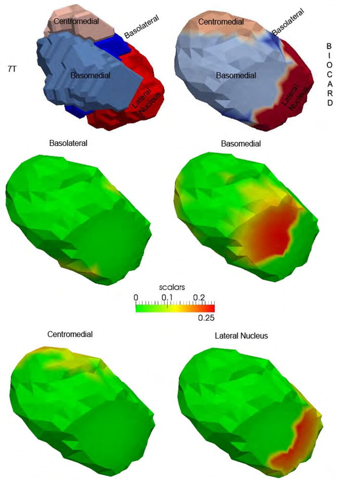
Top row shows the 7T high field amygdala template (left) with four subfields defined from the 0.8mm isotropic 7T MRI and the subfields transferred to the 1.5T population template (right). Middle and bottom row shows the statistical results (Fig. 2) for the template partitioned into the four basolateral, basomedial, centromedial, and lateral nucleus subfields. The reconstruction is shown in the same orientation as Figs. 1–2.

Discussion

A preliminary study of amygdalar shape analysis in a unique cohort has revealed volumetric changes as well as non-uniform shape changes in the amygdala in MCI and AD. The volumetric changes are consistent with those observed in a recent study [20] of two large samples in MCI and AD and may be correlated with that of the hippocampus in the early stages of the disease. The non-uniform changes in shape may explain the variation in volume noted [20] in the relatively few neuroimaging studies of amygdala in MCI and AD. By leveraging a high-field amygdala atlas, significantly atrophied subregions were located specifically in the basomedial and lateral subfields. This is consistent with the histopathological findings with greatest cell packing density loss in the medial region and some loss in the lateral region [16]. The lateral area has also been noted in recent shape analysis by Cavedo et al. [22] and Qiu et al. [21]. The former study is pertinent since a diffeomorphic approach was applied to a small sample and a parcellated amygdala atlas albeit at 3T was used. Thus application of advanced computational anatomy methods can detect atrophy in legacy data such as this BIOCARD study.

These preliminary findings warrant further investigation in several directions. First the bias with respect to the single atlas segmentation could be minimized by using a multi-atlas. Second splitting the disease cohort into two may reveal different patterns of atrophy especially in the early stages of MCI and AD. Despite the small size, atrophied subregions of the amygdala could be detected with p-values based on family-wise error rates which unlike false discovery rates have the advantage of not requiring additional assumptions on the data such as independence or positive dependence. However, caution must be taken when interpreting changes in the exterior shape of a structure with respect to loss of neurons or other processes within the structure. Third the matching of the subfields from the high field atlas to the 1.5T population template needs to be verified especially in regards to the stability of the anatomical boundary definitions. However, a key point is that diffeomorphic transference of the subfields ensures anatomical consistency. Finally, given the temporal lobe circuitry model of the degenerative processes in MCI and AD, it will be necessary to correlate shape changes in the amygdala with that in the hippocampus, entorhinal cortex and other structures.

Future studies will explore the temporal lobe circuitry affected in MCI and AD. Such expanded studies may provide additional biomarkers to that of the hippocampus in the early stages of MCI and AD.

References

- 1.Jernigan TL, et al. Cerebral Structure on Mri.2. Specific Changes in Alzheimers and Huntingtons Diseases. Biological Psychiatry. 1991;29(1):68–81. doi: 10.1016/0006-3223(91)90211-4. [DOI] [PubMed] [Google Scholar]
- 2.Braak H, Braak E. Neuropathological stageing of Alzheimer-related changes. Acta Neuropathol. 1991;82(4):239–59. doi: 10.1007/BF00308809. [DOI] [PubMed] [Google Scholar]
- 3.Arnold SE, et al. The topographical and neuroanatomical distribution of neurofibrillary tangles and neuritic plaques in the cerebral cortex of patients with Alzheimer’s disease. Cereb Cortex. 1991;1(1):103–16. doi: 10.1093/cercor/1.1.103. [DOI] [PubMed] [Google Scholar]
- 4.Price JL, Morris JC. Tangles and plaques in nondemented aging and “preclinical” Alzheimer’s disease. Ann Neurol. 1999;45(3):358–68. doi: 10.1002/1531-8249(199903)45:3<358::aid-ana12>3.0.co;2-x. [DOI] [PubMed] [Google Scholar]
- 5.Jack CR, Jr, et al. Brain beta-amyloid measures and magnetic resonance imaging atrophy both predict time-to-progression from mild cognitive impairment to Alzheimer’s disease. Brain. 2010;133(11):3336–48. doi: 10.1093/brain/awq277. [DOI] [PMC free article] [PubMed] [Google Scholar]
- 6.McEvoy LK, et al. Mild cognitive impairment: baseline and longitudinal structural MR imaging measures improve predictive prognosis. Radiology. 2011;259(3):834–43. doi: 10.1148/radiol.11101975. [DOI] [PMC free article] [PubMed] [Google Scholar]
- 7.Bossa M, Zacur E, Olmos S. Statistical analysis of relative pose information of subcortical nuclei: application on ADNI data. Neuroimage. 2011;55(3):999–1008. doi: 10.1016/j.neuroimage.2010.12.078. [DOI] [PMC free article] [PubMed] [Google Scholar]
- 8.Roh JH, et al. Volume reduction in subcortical regions according to severity of Alzheimer’s disease. J Neurol. 2011;258(6):1013–20. doi: 10.1007/s00415-010-5872-1. [DOI] [PubMed] [Google Scholar]
- 9.Qiu A, et al. Basal Ganglia Shapes Predict Social Communication, and Motor Dysfunctions in Boys With Autism Spectrum Disorder. Journal of the American Academy of Child & Adolescent Psychiatry. 2010;49:539–551. doi: 10.1016/j.jaac.2010.02.012. [DOI] [PubMed] [Google Scholar]
- 10.Csernansky J, et al. Hippocampal morphometry in schizophrenia by high dimensional brain mapping. Proc Natl Acad Sci USA. 1998;95:11406–11411. doi: 10.1073/pnas.95.19.11406. [DOI] [PMC free article] [PubMed] [Google Scholar]
- 11.Csernansky J, et al. Early {DAT} is distinguished from aging by high-dimensional mapping of the hippocampus. Neurology. 2000;55:1636–1643. doi: 10.1212/wnl.55.11.1636. [DOI] [PubMed] [Google Scholar]
- 12.Wang L, et al. Large deformation diffeomorphism and momentum based hippocampal shape discrimination in dementia of the Alzheimer type. IEEE transactions on medical imaging. 2007;26:462–70. doi: 10.1109/TMI.2005.853923. [DOI] [PMC free article] [PubMed] [Google Scholar]
- 13.Ashburner J, et al. Computer-assisted imaging to assess brain structure in healthy and diseased brains. Lancet Neurol. 2003;2(2):79–88. doi: 10.1016/s1474-4422(03)00304-1. [DOI] [PubMed] [Google Scholar]
- 14.Thompson PM, et al. Mapping hippocampal and ventricular change in Alzheimer disease. Neuroimage. 2004;22(4):1754–66. doi: 10.1016/j.neuroimage.2004.03.040. [DOI] [PubMed] [Google Scholar]
- 15.Arriagada PV, et al. Neurofibrillary tangles but not senile plaques parallel duration and severity of Alzheimer’s disease. Neurology. 1992;42(3 Pt 1):631–9. doi: 10.1212/wnl.42.3.631. [DOI] [PubMed] [Google Scholar]
- 16.Herzog AG, Kemper TL. Amygdaloid changes in aging and dementia. Arch Neurol. 1980;37(10):625–9. doi: 10.1001/archneur.1980.00500590049006. [DOI] [PubMed] [Google Scholar]
- 17.Scott SA, DeKosky ST, Scheff SW. Volumetric atrophy of the amygdala in Alzheimer’s disease: quantitative serial reconstruction. Neurology. 1991;41(3):351–6. doi: 10.1212/wnl.41.3.351. [DOI] [PubMed] [Google Scholar]
- 18.Scott SA, et al. Amygdala cell loss and atrophy in Alzheimer’s disease. Ann Neurol. 1992;32(4):555–63. doi: 10.1002/ana.410320412. [DOI] [PubMed] [Google Scholar]
- 19.Tsuchiya K, Kosaka K. Neuropathological study of the amygdala in presenile Alzheimer’s disease. J Neurol Sci. 1990;100(1–2):165–73. doi: 10.1016/0022-510x(90)90029-m. [DOI] [PubMed] [Google Scholar]
- 20.Poulin SP, et al. Amygdala atrophy is prominent in early Alzheimer’s disease and relates to symptom severity. Psychiatry Res. 2011;194(1):7–13. doi: 10.1016/j.pscychresns.2011.06.014. [DOI] [PMC free article] [PubMed] [Google Scholar]
- 21.Qiu A, et al. Regional shape abnormalities in mild cognitive impairment and Alzheimer’s disease. Neuroimage. 2009;45:656–661. doi: 10.1016/j.neuroimage.2009.01.013. [DOI] [PMC free article] [PubMed] [Google Scholar]
- 22.Cavedo E, et al. Local amygdala structural differences with 3T MRI in patients with Alzheimer disease. Neurology. 2011;76(8):727–33. doi: 10.1212/WNL.0b013e31820d62d9. [DOI] [PMC free article] [PubMed] [Google Scholar]
- 23.Munn MA, et al. Amygdala volume analysis in female twins with major depression. Biological Psychiatry. 2007;62(5):415–422. doi: 10.1016/j.biopsych.2006.11.031. [DOI] [PMC free article] [PubMed] [Google Scholar]
- 24.Umeyama S. Least-Squares Estimation of Transformation Parameters between 2 Point Patterns. Ieee Transactions on Pattern Analysis and Machine Intelligence. 1991;13(4):376–380. [Google Scholar]
- 25.Joshi S, Miller MI. Landmark Matching Via Large Deformation Diffeomorphisms. IEEE TRANSACTIONS ON IMAGE PROCESSING. 2000;9(8):1357–1370. doi: 10.1109/83.855431. [DOI] [PubMed] [Google Scholar]
- 26.Beg MF, et al. Computing large deformation metric mappings via geodesic flows of diffeomorphisms. International Journal of Computer Vision. 2005;61(2):139–157. [Google Scholar]
- 27.Ma J, Miller M, Younes L. A Bayesian Generative Model for Surface Template Estimation. International Journal of Biomedical Imaging. 2010;2010 doi: 10.1155/2010/974957. [DOI] [PMC free article] [PubMed] [Google Scholar]
- 28.Vaillant M, Glaunes J. IPMI2005. Springer-Verlag New York Inc; 2005. Surface matching via currents. [DOI] [PubMed] [Google Scholar]
- 29.Younes L. Shapes and diffeomorphisms. New York: Springer; 2010. [Google Scholar]
- 30.Nichols T, Hayasaka S. Controlling the familywise error rate in functional neuroimaging: a comparative review. Statistical Methods in Medical Research. 2003;12(5):419–446. doi: 10.1191/0962280203sm341ra. [DOI] [PubMed] [Google Scholar]
- 31.Miller MI, Qiu A. The emerging discipline of Computational Functional Anatomy. Neuroimage. 2009;45(1 Suppl):S16–39. doi: 10.1016/j.neuroimage.2008.10.044. [DOI] [PMC free article] [PubMed] [Google Scholar]
- 32.Mai JK, Assheuer J, Paxinos G. Atlas of the human brain. 2. viii. Amsterdam; Boston: Elsevier Academic Press; 2004. p. 246. [Google Scholar]